| Issue |
A&A
Volume 551, March 2013
|
|
|---|---|---|
| Article Number | A105 | |
| Number of page(s) | 13 | |
| Section | The Sun | |
| DOI | https://doi.org/10.1051/0004-6361/201220543 | |
| Published online | 01 March 2013 | |
Correlations between sunspots and their moat flows⋆
Kiepenheuer-Institut für Sonnenphysik,
Schöneckstr. 6,
79104
Freiburg,
Germany
e-mail: This email address is being protected from spambots. You need JavaScript enabled to view it.
; This email address is being protected from spambots. You need JavaScript enabled to view it.
Received:
11
October
2012
Accepted:
19
December
2012
Abstract
Context. The presence of the moat flow around sunspots is intimately linked to the mere existence of sunspots.
Aims. We characterize the moat flow (MF) and Evershed flow (EF) in sunspots to enhance our knowledge of sunspot structures and photospheric flow properties.
Methods. We calibrated HMI synoptic Doppler maps and used them to analyze 3 h time averages of 31 circular, stable, and fully developed sunspots at heliocentric angles of some 50°. Assuming axially symmetrical flow fields, we infer the azimuthally averaged horizontal velocity component of the MF and EF from 51 velocity maps. We studied the MF properties (velocity and extension) and elaborate on how these components depend on sunspot parameters (sunspot size and EF velocity). To explore the weekly and monthly evolution of MFs, we compare spots rotating from the eastern to western limbs and spots that reappear on the eastern limb.
Results. Our calibration procedure of HMI Doppler maps yields reliable and consistent results. In 3 h averages, we find the MF decreases on average from some 1000 ± 200 m/s just outside the spot boundary to 500 m/s after an additional 4 Mm. The average MF extension lies at 9.2 ± 5 Mm, where the velocity drops below some 180 m/s. Neither the MF velocity nor its extension depend significantly on the sunspot size or EF velocity. But, the EF velocity does show a tendency to be enhanced with sunspot size. On a time scale of a week and a month, we find decreasing MF extensions and a tendency for the MF velocity to increase for strongly decaying sunspots, whereas the changing EF velocity has no impact on the MF.
Conclusions. On 3 h averages, the EF velocity scales with the size of sunspots, while the MF properties show no significant correlation with the EF or with the sunspot size. This we interpret as a hint that the physical origins of EF and MF are distinct.
Key words: sunspots / Sun: activity / Sun: photosphere / Sun: rotation / convection / techniques: radial velocities
Appendix A is available in electronic form at http://www.aanda.org
© ESO, 2013
1. Introduction
As complex magnetic formations, sunspots strongly affects the photospheric dynamics of the granular convective pattern of the plasma in which they are embedded. They suppress the upward propagation of heat in the magnetic core, seen as the cooler and therefore darker umbra, and they harbor the well-known penumbral Evershed flow observed as a radially outwards-directed, horizontal flow in the photospheric layers. In photospheric observations this leads to a blueshift and blueward asymmetry of the spectral line for penumbral filaments facing the center of the solar disk and a redshift and redward asymmetry for filaments facing the solar limb (e.g., Evershed 1909; Maltby 1964; Schlichenmaier et al. 2004). In general, the line shift, as well as the asymmetry, increases from the inner to the outer penumbra. In photospheric layers the Evershed flow is close to horizontal with maximum inclinations of 5° to 10°, exhibiting downward flows in the outer penumbra (e.g., Michard 1951; Balthasar et al. 1996; Schlichenmaier & Schmidt 2000; Franz & Schlichenmaier 2009). Average horizontal velocities are in the range of 3−4 km s-1 (Shine et al. 1994), but can exceed 6 km s-1 or more on small scales (e.g., Rouppe van der Voort 2002; Bellot Rubio et al. 2003a). The Evershed flow seems to stop abruptly at the white light boundary of the spot (Wiehr & Degenhardt 1992; Schlichenmaier & Schmidt 1999), which is in line with downward flows in the outer penumbra. Only a small fraction of the flow continues to flow into the magnetic canopy that surrounds the spot (Rezaei et al. 2006).
Whereas the Evershed flow (EF) is magnetized (e.g., Schlichenmaier & Collados 2002), the annular region around fully-fledged sunspots, called the moat cell, is largely nonmagnetic. It harbors the moat flow (MF), a radially oriented outflow of plasma adjacent to the outer penumbral boundary. Embedded in these motions, small, moving magnetic features (MMFs) migrate away from the sunspot (Sheeley 1969, 1972; Vrabec 1971; Harvey & Harvey 1973). The existence of both the MF and the EF depend on the presence of a penumbra (Vrabec 1974). Consequently, the moat flow can only be observed for sunspot sides with a well-developed penumbra and lacks pores (Sobotka et al. 1999).
The moat flow develops immediately after the formation of a penumbra (Pardon et al. 1979; Schlichenmaier et al. 2010) and was observed even after the decay of the penumbra (Verma et al. 2012). The MF is present as a stationary flow through the spot’s lifetime, which varies between several weeks to several months (see, e.g., Solanki 2003): Sobotka & Roudier (2007) do not find any significant variations in the MF within half a day. During the initiation of the MF, the magnetic components in the vicinity of the sunspot are pushed to the periphery and leave the moat cell largely nonmagnetic with single MMFs. The extension of the moat field reaches between 10 Mm to 20 Mm from the penumbral boundary for small sunspots and can be roughly twice the spot radius for larger spots (Brickhouse & Labonte 1988), but Sobotka & Roudier (2007) find no such correspondence.
The moat flow velocity ranges between 0.5 km s-1 to 1 km s-1 and can be seen by tracking the bright granular features (e.g., Rimmele 1997; Vargas Domínguez et al. 2007; Balthasar & Muglach 2010) or Doppler shift measurements (Balthasar et al. 1996). That the MF consists of migrating granules, indicates that the MF is as nonmagnetic as granules, i.e., largely nonmagnetic.
Also helioseismic measurements have revealed the existence of the MF as an outflow extending up to 30 Mm with a maximum velocity of 1 km s-1 just next to the penumbral boundary (Gizon et al. 2000) in the first 2 Mm of the solar surface. According to recent studies (Sun et al. 1997; Gizon et al. 2009; Featherstone et al. 2011), the MF is also detectable in deeper layers, but has slower speeds compared to surface measurements.
Cabrera Solana et al. (2006) suggest that a link exists between EF and MMFs. Magnetic velocity packages, called the Evershed clouds inside the penumbra (Shine et al. 1994; Rimmele 1994; Cabrera Solana et al. 2007) propagate outwards to the extension of penumbral filaments and the moat region where they are embedded as MMFs. MMFs can travel from the penumbra into the vicinity of the sunspot (Sainz Dalda & Martínez Pillet 2005; Sainz Dalda & Bellot Rubio 2008a,b). Also Schlichenmaier (2002) proposes a scenario that is consistent with observed MMFs. In this way, a magneto-convective overshoot instability in an Evershed flux tube leads to the migrating feature in the MF region. There is still discordance about a link between the EF and MF. Vargas Domínguez et al. (2007) observed irregular sunspots and found that the moat flow is only present in radial extensions of penumbral filaments, but not perpendicular to them. This indicates that the MF is an extension of the EF. However, this seems to be impossible since the EF is magnetized, while the MF is intrinsically unmagnetic, as mentioned above.
In this paper, we analyze the EF and MF and elaborate on a possible link between the two. To that end, we utilize Doppler shift measurements of HMI. In Sect. 2 we perform a thorough calibration of HMI Doppler maps. In Sect. 3 we describe the criteria for data selection and the method we used to analyze the flow properties. In Sect. 4 we present our results for the flow properties and elaborate on correlations between spot and MF properties and on how they change during the evolution of a spot. The statistics are based on 51 maps constructed from 31 different spots. The data sets we used and the radial dependencies of the flow velocity of all spots, which form the basis of our analysis, are given in the appendix. In Sect. 5, we discuss the present understanding of MFs in the context of our results and summarize our results and conclusions.
2. Calibration of HMI Doppler maps
Data:
our work is based on synoptic 720 s intensity maps and Doppler maps1 in the Fe i spectral line at 6173.3 Å from the JSOC webpage recorded by the Helioseismic Magnetic Imager (HMI) of the Solar Dynamics Observatory (SDO) up to maximum values of ±6.5 km s-1 and a spatial resolution of ≈0.5″/px.
Calibration by subtracting systematic components:
to yield undisturbed flow velocities relative to the solar surface, we need to define a
rest frame (v = 0). To this end, we construct a time averaged velocity
map, ⟨ v(x,y) ⟩ t, in which
the effects of granulation, oscillations, and supergranulation are removed. This average
is composed of three systematic, large-scale components:  (1)The first term is the
center-to-limb variation in the convective blueshift, vclv. It
is radially symmetrical and is several hundred m/s, depending on the distance,
r, (or heliocentric angle θ) to disk center. The
second term is the differential rotation, vrot. It is axially
symmetrical with velocities up to ±2000 m/s with respect to the
meridian. The values depend on the distance d from the meridian, the
latitude l and the inclination B0 of the
rotation axis, which varies annually between ±7.27°. The third term is a
nonsymmetrical residual, vres, with velocities up to
±150 m/s, which contains instrumental effects and other systematic
flow fields of smaller magnitude. The large-scale meridional flow with velocities of less
than 20 m/s can be neglected for our sunspot studies, and if existing, it is included in
these three components. In the next four sections we determine the four terms of Eq.
(1).
(1)The first term is the
center-to-limb variation in the convective blueshift, vclv. It
is radially symmetrical and is several hundred m/s, depending on the distance,
r, (or heliocentric angle θ) to disk center. The
second term is the differential rotation, vrot. It is axially
symmetrical with velocities up to ±2000 m/s with respect to the
meridian. The values depend on the distance d from the meridian, the
latitude l and the inclination B0 of the
rotation axis, which varies annually between ±7.27°. The third term is a
nonsymmetrical residual, vres, with velocities up to
±150 m/s, which contains instrumental effects and other systematic
flow fields of smaller magnitude. The large-scale meridional flow with velocities of less
than 20 m/s can be neglected for our sunspot studies, and if existing, it is included in
these three components. In the next four sections we determine the four terms of Eq.
(1).
2.1. Construction of a time-averaged velocity map: ⟨v(x, y)⟩ t
In velocity maps, supergranules produce a redshift on the limb side and a blueshift on the opposite side when they are off disk center. Because a supergranule migrates across the disk its average velocity signal vanishes when it is next to the equator, since blueshifts are eliminated by the following redshifts. However, close to the poles, the blueshifts and redshifts are separated in latitude such that a single supergranule leaves noticeable traces in the Doppler map. To diminish these traces a long time series is necessary. In our case we have averaged 720 s Doppler maps of 61 entire days (a total of 7320 maps) between June and December 2010, shown in the left hand panel of Fig. 1.
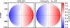 |
Fig. 1 Left panel: averaged velocity map, ⟨ v(x,y) ⟩ t = 61 days, with maximum blueshifts (eastern limb) and redshifts (western limb) with some 2 km s-1. The axes are given in arcsec. Right panel: reduced velocity map, ⟨ v(x,y) ⟩ t − vclv. |
In order not to spoil the time average by active regions, we have masked regions according to the darkening in the continuum intensity and replaced the content of the mask in the Doppler map by the velocities on the opposite side of the heliocentric equator. Thanks to the solar activity minimum, this method was appropriate. For consistency, we normalized the solar radius of all Doppler maps and eliminated the respective observer motion2 relative to the Sun. Since we favored time periods with inclination B0 ≈ 0°, the obtained velocity map ⟨ v(x,y) ⟩ t = 61 days should serve as a good basis for modeling the systematic components named in Eq. (1). In ⟨ v(x,y) ⟩ t the velocity at disk center is about 50 m/s.
2.2. Radially symmetrical velocity component: vclv(r)
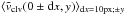
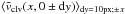
As seen in the left hand panel of Fig. 1, the LOS velocity of the solar rotation, which should be zero for the meridian and axially symmetrical with respect to the centerlines, is deformed. This deformation along the meridian contains the center-to-limb variation (CLV) of the convective blueshift and the meridional flow. To determine the sum of both effects a priori (without knowing the differential rotation), we decided to use the average, ⟨ v(0 ± dx,y) ⟩ t; dx = 10px; ±y, of a 20-pixel wide stripe along the meridian of ⟨ v(x,y) ⟩ t with respect to the distance, r, to the disk center as shown in Fig. 2a. Assuming radial symmetry, the curves of the northern and southern hemispheres are averaged. The resulting ⟨ v(0,y) ⟩ t is fitted by a 8th-order polynomial, vclv(y). The curve runs from +50 m/s at the disk center to −60 m/s at some 700″ and strong redshifts exceeding 300 m/s at the solar limb. This CLV is in good accordance with recent studies of the CLV of the Fe i line (e.g., Balthasar 1985; Cruz Rodríguez et al. 2011). As the up- and downturns, which are caused by the supergranular migration at higher latitudes, are on the order of some 30 m/s, we neglect the impact of the meridional flow3 on vclv(y) and further calibrations. We use the polynomial vclv(y) to create a radially symmetrical CLV model, vclv(r), as displayed in Fig. 2b.
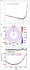 |
Fig. 2 a) Average CLV,
⟨ v(0,y) ⟩ t,
along the meridional centerline with an 8th-order polynomial fit,
vclv(y) (red curve) in m/s against
the distance y to the disk center in arcsec. b)
Calibrated, radially symmetrical CLV model,
vclv(r), with axis given in arcsec.
c) Convective blueshift,
vb(r), in
|

Since the convective blueshift is the result of the bigger impact of hot upwards moving granules than the cool, downwards directed, intergranular fraction on a spatially averaged solar surface, the line shift depends on the observed spectral line and the line of sight. According to calculations based on the Liège atlas (Delbouille et al. 1990), the convective blueshift of the Fe i spectral line at 6173.3 Å in the center is vb = −305 m/s. For observational studies in Sect. 3, we have to offset vclv(r) by voff ≈ −350 m/s to obtain the convective blueshift, vb(r), with its CLV.
After the calibration of
vrot(d,l,B0)
and vres(x,y) in Sects. 2.3 and 2.4 we can check the
accuracy of the data calibration by computing the CLV velocity map a posteriori:
 Then,
we compare the CLV in the meridional and equatorial directions, i.e.
Then,
we compare the CLV in the meridional and equatorial directions, i.e.
 and
and
 .
The curves are displayed in Fig. 2c and closely
resemble each other. The velocities were offset by voff to
achieve the run from
vb(cosθ = 1) = −305 m/s
to
vb(cosθ = 0.8...0.6) ≈ −400 m/s
(preferred spot location) and lower velocities at the solar limb. While the equatorial
direction exhibits minor fluctuations, the meridional direction displays stronger
fluctuations owing to the residuals of supergranules. The difference between both curves
shown in the upper part of Fig. 2c reveals an rms
smaller than 10 m/s in low latitudes. The dashed green curve in Fig. 2c results from synthetic profiles for Fe i 6173.3 Å based on
COBOLD simulations (Freytag et al. 2012; Beeck et al. 2012). The synthetic curve differs by less
than 100 m/s, so is in good qualitative agreement with our measurements.
.
The curves are displayed in Fig. 2c and closely
resemble each other. The velocities were offset by voff to
achieve the run from
vb(cosθ = 1) = −305 m/s
to
vb(cosθ = 0.8...0.6) ≈ −400 m/s
(preferred spot location) and lower velocities at the solar limb. While the equatorial
direction exhibits minor fluctuations, the meridional direction displays stronger
fluctuations owing to the residuals of supergranules. The difference between both curves
shown in the upper part of Fig. 2c reveals an rms
smaller than 10 m/s in low latitudes. The dashed green curve in Fig. 2c results from synthetic profiles for Fe i 6173.3 Å based on
COBOLD simulations (Freytag et al. 2012; Beeck et al. 2012). The synthetic curve differs by less
than 100 m/s, so is in good qualitative agreement with our measurements.
2.3. Differential rotation: vrot(d, l, B0)
Since the rotation velocity is differential on the solar surface and depends on the line of sight (LOS), we have to generate a specific, axially symmetrical solar rotation model, vrot(d,l,B0), with respect to the distance, d, from the meridian, the latitude, l, and the inclination, B0, of the rotation axis.
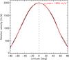 |
Fig. 3 Absolute rotation velocities, vrot(l,B0 = 0), in m/s (black curve) on the solar surface for latitudes up to l = ±80° fitted by Ω(l) (red curve) and an equatorial maximum of Ω(0) = 1992 m/s. |
We start out with the time-averaged velocity map reduced by the radially symmetrical component, i.e. ⟨ v(x,y) ⟩ t − vclv(r), displayed in the right hand panel of Fig. 1. We determine the absolute latitudinal velocity, vrot(l) for B0 = 0°, by performing linear regressions for the LOS velocities along latitudinal cuts, v(d/Rl), with Rl being the distance of the solar limb from the meridian: vrot(d,l) = vrot(l)·(d/Rl). Figure 3 shows the latitudinal dependence, vrot(l).
To compare our rotation model with literature values, we follow Stix (2002) and approximate
vrot(l) by  (2)The approximation,
Ω(l), is plotted in Fig. 3. We
obtained a differential decrease to higher latitudes. The equatorial maximum,
A = 14.10 ± 0.03°/day, corresponds to
Ω(0) = 1992 m/s. The coefficients
B = −9.0°/day and
C = −2.5°/day have standard deviations
on the order of 0.1°/day. Since the result depends on the method of measurement
(see: Stix 2002), we compared our rotational
velocity with the Doppler shift measurements of Snodgrass
(1984) who obtained an equatorial rate of
A = 14.05 ± 0.01°/day or
Ω(0) = 1975 m/s. This is in good accordance with our findings.
However, compared to Snodgras coefficients,
B = −1.49°/day and
C = −2.61°/day with deviations on the
order of some 0.1°/day, we obtained a stronger decrease in
the rotational velocity to higher latitudes.
(2)The approximation,
Ω(l), is plotted in Fig. 3. We
obtained a differential decrease to higher latitudes. The equatorial maximum,
A = 14.10 ± 0.03°/day, corresponds to
Ω(0) = 1992 m/s. The coefficients
B = −9.0°/day and
C = −2.5°/day have standard deviations
on the order of 0.1°/day. Since the result depends on the method of measurement
(see: Stix 2002), we compared our rotational
velocity with the Doppler shift measurements of Snodgrass
(1984) who obtained an equatorial rate of
A = 14.05 ± 0.01°/day or
Ω(0) = 1975 m/s. This is in good accordance with our findings.
However, compared to Snodgras coefficients,
B = −1.49°/day and
C = −2.61°/day with deviations on the
order of some 0.1°/day, we obtained a stronger decrease in
the rotational velocity to higher latitudes.
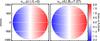 |
Fig. 4 Computed differential rotation maps, vrot(d,l,B0 = 0°) (left panel) and vrot(d,l,B0 = 7.27°) (right panel), with maximum velocities vrot(l = 0,B0 = 0°) = 1992 m/s and vrot(l = 0,B0 = 7.27°) = 1976 m/s, spatially displayed in arcsec. |
The differential rotation model, vrot(d,l,B0), displayed as an example in Fig. 4 for B0 = 0° (left panel) and B0 = 7.27° (right panel), generates the LOS velocities for every position on the solar disk according to the annually varying B0 = ±7.27°.
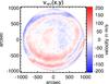 |
Fig. 5 Residual velocity map, vres(x,y), with axis given in arcsec. |
2.4. Residual velocity map: vres(x, y)
Augural annular patterns (see Fig. 1) indicate a
systematical, nonsymmetrical residual,
vres(x,y), that contains instrumental
effects and other systematic flow fields of smaller magnitude. Subtracting
vclv and vrot from the 61
dayaverage, ⟨ v ⟩ t, we obtain the residual
nonsymmetrical velocity map:  (3)which is displayed in
Fig. 5. Our result agrees well with the HMI
calibration studies of Howe et al. (2011) and Centeno et al. (2011). Several large circular patterns
and smaller interference rings were checked as spatially fixed with velocities varying
between ±150 m/s. The residual map is subtracted a priori for all Doppler maps in Sect.
3. Changes in time are expected to have small
amplitudeso will not affect our analysis of horizontal flow velocities.
(3)which is displayed in
Fig. 5. Our result agrees well with the HMI
calibration studies of Howe et al. (2011) and Centeno et al. (2011). Several large circular patterns
and smaller interference rings were checked as spatially fixed with velocities varying
between ±150 m/s. The residual map is subtracted a priori for all Doppler maps in Sect.
3. Changes in time are expected to have small
amplitudeso will not affect our analysis of horizontal flow velocities.
3. Data selection and analysis
Overview:
in this section, we analyze the sunspot moat flow and Evershed flow in the solar photosphere by the calibrated 720 s Doppler maps recorded by HMI. We have selected circular sunspots and constructed 3 h time averages (out of 15 such Doppler maps) of the field of view (FOV). By doing this, we reduce the amplitudes of granulation and oscillation (see Sect. 3.1). We analyze the flow field in the penumbra and in the surrounding moat cell.
 |
Fig. 6 a) 720 s intensity map and b) corresponding 720 s
velocity map, |

3.1. Data selection and preprocessing:
The moat flow is coupled to the presence of a penumbra and follows the direction of the penumbral filaments. Thus, we searched for sunspots with a fully-fledged, circular penumbra and found 31 applicable, single sunspots in a slight decay4 in the time between June 2010 and January 2012. The selected sunspots vary in size between 9 Mm and 22 Mm and are listed in Table A.1 of the appendix. A contour of the outer penumbra for each spot is determined by means of an intensity threshold for a spatially averaged image. The center of a sunspot is determined as the center-of-gravity of all points inside its penumbral contour.
To analyze predominantly horizontal flows with LOS Doppler maps, we selected the observing position of the sunspot center at heliocentric angles of some θ ≈ 50°. There, the LOS component of the horizontal flow is significant, while the calibration uncertainties that increase towards the solar limb are still small.
Each sunspot FOV from the size of 301 × 301 px is tracked by its averaged center,
(xc,yc), for 15
successive 720 s intensity maps (Fig. 6a), while the
respective Doppler maps, vdop(x,y), are
calibrated by  (4)to obtain velocity
maps,
(4)to obtain velocity
maps,  , (Fig.
6b) free of all systematical velocity components
(described in Sect. 2), but the surface
convection.voff describes the offset of the convective
blueshift and its CLV (Fig. 2c) to values around
−400 m/s at the chosen observing position.
, (Fig.
6b) free of all systematical velocity components
(described in Sect. 2), but the surface
convection.voff describes the offset of the convective
blueshift and its CLV (Fig. 2c) to values around
−400 m/s at the chosen observing position.
The sunspot and flow properties are stable within three hours. To diminish 5-min oscillations and granulation, we averaged the tracked and aligned sunspot FOVs (201 × 201 px) of all the 15 successive velocity maps and refer to this 3 h average as v3h (Figs. 6c–h). Likewise, the received LOS velocities are adapted for an average heliocentric angle, θ. For better illustrating the MF, the 3 h average is shown here with a masked umbra and penumbra.
We studied the weekly evolution of the observed components by tracking 20 sunspots near the eastern limb to a second proper position (θ ≈ 50°) after some 6 to 8 days and compared the results of both v3h analysis. As this was not possible for 11 of 31 spots, we achieve a sample of 51 velocity maps. Tracking three long-lasting sunspots across the far side of the Sun, they reappear at the eastern front side (Table A.1: No. 4 → 6, 7 → 9, 11 → 13; Figs. 6e–h) which allows us to study the monthly evolution.
3.2. Method of flow analysis
We analyze flow fields of fully calibrated velocity maps,
v3h, by applying a method that determines the azimuthally
averaged flow properties (Schlichenmaier & Schmidt
2000). In this way, we assume axially symmetrical flow fields for circular
sunspots with a fully developed penumbra. The foreshortening effects of a circular sunspot
at a certain heliocentric angle, θ, cause the elliptical shape as shown
for AR11084 (Figs. 6a–d). To observe the spatial
velocity dependency of the flow fields, we use an automatic procedure that generates
ellipses as foreshortened circles (with radii, r, in px) based on the
heliocentric angle and rotated according to their position on the disk. The LOS
velocities, vLOS(r,φ), along the ellipses are
read out according to their circular angle, φ, as shown in Fig. 7 for distances
r = RS + 5 (upper panel) and
r = RS + 10 (lower panel) from the
spot center. The sunspot radius is automatically determined by the minimal deviation of
the ellipse to the penumbral contour for every 720 s intensity map and averaged for the 3
h period. A manual fine adjustment was added for irregularities. The LOS velocities,
vLOS(r,φ), were fitted by a sine function:
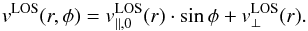 (5)The amplitude,
 , is the LOS
component of the horizontal flow velocity
, is the LOS
component of the horizontal flow velocity 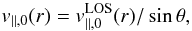 (6)at the heliocentric
angle, θ. The axial offset,
(6)at the heliocentric
angle, θ. The axial offset,  , is the
vertical flow component.
, is the
vertical flow component.
3.3. Moat flow
We analyze the moat flow in the vicinity of the sunspots for the fully calibrated velocity maps, v3h (listed in Table A.1).
3.3.1. Moat flow velocity
The moat flow is an outwardly directed flow, which is predominantly horizontal.We present the flow field analysis for the velocity map, v3h, of AR11084 (Figs. 6c, d; Table A.1: No. 1b). The sunspot in the FOV center with an average spot radius of RS = 31 px ≈ 11.2 Mm at θ = 51° exhibits a distinct moat flow surrounding the sunspot with LOS velocities up to −1000 m/s for the blueshifted side facing the disk center and +1000 m/s for the redshifted limb side indicated by an arrow. The outer vicinity of the sunspot features supergranular flow cells.
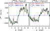 |
Fig. 7 Angular LOS velocities, vLOS(r,φ),
in m/s along the elliptical projection for θ = 51° of
circles with radius r = RS + 5 px
(left panel) and
r = RS + 10 px (right
panel) fitted by a sine curve (green, solid line) according to Eq.
(5). The amplitude,
|

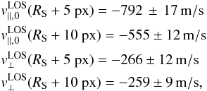
Comparing the velocity components of the MF in a distance of 5 px and 10 px from the sunspot (see Fig. 7)
 the
most prominent result is the decrease in by more
than 230 m/s within these 2 Mm. The upper panel of Fig. 8 shows the continuous run of the horizontal flow velocities,
v∥ ,0(r), at
θ = 51° (see Eq. (6)), from the spot center to a distance of 25 Mm. The MF has a strong monotone
decrease with increasing distance from 1150 m/s just outside the
penumbra to 600 m/s after additional 3 Mm and 250 m/s after 6 Mm.
the
most prominent result is the decrease in by more
than 230 m/s within these 2 Mm. The upper panel of Fig. 8 shows the continuous run of the horizontal flow velocities,
v∥ ,0(r), at
θ = 51° (see Eq. (6)), from the spot center to a distance of 25 Mm. The MF has a strong monotone
decrease with increasing distance from 1150 m/s just outside the
penumbra to 600 m/s after additional 3 Mm and 250 m/s after 6 Mm.
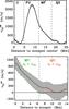 |
Fig. 8 Upper panel: horizontal flow velocities,
v∥ ,0(r), in m/s
for the distance, r, from the spot center in Mm. Error bars
represent the standard deviation. Dashed vertical lines mark the boundaries
between umbra (U), penumbra (PU), and moat flow region (MF) and the quiet Sun
(QS). Lower panel: horizontal LOS velocity,
|
The vertical flow component of MF and EF depends on the choice of the rest frame. Our
rest frame is determined by the convective blueshift of nonmagnetic convection. Since
the MF region is not completely free of magnetic fields, it may change the convective
blueshift by an unknown amount. Therefore, no accurate analysis of the vertical MF
component,  , can be given. Also, the
inclination of the MF could not be reliably determined owing to the dependence on the
vertical flow component (Schlichenmaier &
Schmidt 2000). However, on the assumption that no effect is caused by magnetic
fields, we can subtract the convective blueshift
vb(r) ≈ −400 m/s
from and obtain absolute
vertical velocities of
, can be given. Also, the
inclination of the MF could not be reliably determined owing to the dependence on the
vertical flow component (Schlichenmaier &
Schmidt 2000). However, on the assumption that no effect is caused by magnetic
fields, we can subtract the convective blueshift
vb(r) ≈ −400 m/s
from and obtain absolute
vertical velocities of  . According to that,
the slight redshift indicates a downward-directed MF. In comparison with horizontal MF
velocities up to
. According to that,
the slight redshift indicates a downward-directed MF. In comparison with horizontal MF
velocities up to  m/s, the
vertical velocity is an order of magnitude less, and therefore it has a minor impact on
the absolute flow velocity.
m/s, the
vertical velocity is an order of magnitude less, and therefore it has a minor impact on
the absolute flow velocity.
3.3.2. Moat flow extension
To detect the size of the MF region, we define the criteria
 to indicate the
end of the detectable MF, whereas the root mean square,
σrms, is calculated for each distance, r,
to the spot by
to indicate the
end of the detectable MF, whereas the root mean square,
σrms, is calculated for each distance, r,
to the spot by 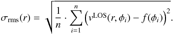 (7)In the lower panel of
Fig. 8, we display
σrms(r) as error bars to the horizontal
LOS velocities. When σrms(r), i.e. the
velocity fluctuation around the sine fit,
f(φi), with circular
angles, φi (see Fig. 7), exceeds the fitted amplitude,
, we define
this distance as the end of the MF region. For the case under consideration, we obtain
an MF, which extends 6.5 Mm into the vicinity of the sunspot. This study of the MF
extension highly depends on σrms, which is about
180 m/s for the 3 h average and which becomes smaller for longer
periods. But, these longer periods cannot guarantee the stability of the observed
components. We therefore believe that our method delivers a good estimate for the MF
extension.
(7)In the lower panel of
Fig. 8, we display
σrms(r) as error bars to the horizontal
LOS velocities. When σrms(r), i.e. the
velocity fluctuation around the sine fit,
f(φi), with circular
angles, φi (see Fig. 7), exceeds the fitted amplitude,
, we define
this distance as the end of the MF region. For the case under consideration, we obtain
an MF, which extends 6.5 Mm into the vicinity of the sunspot. This study of the MF
extension highly depends on σrms, which is about
180 m/s for the 3 h average and which becomes smaller for longer
periods. But, these longer periods cannot guarantee the stability of the observed
components. We therefore believe that our method delivers a good estimate for the MF
extension.
3.4. Evershed flow
Also the well-known penumbral Evershed flow is a predominantly horizontal flow. In our analysis we assume it as axially symmetrical. In Fig. 8 (upper panel), we display the radial dependence of the horizontal flow component of AR11084 (see Fig. 6c) based on v3h. The inner penumbral boundary is determined as the average extension of the umbral darkening in all 720 s intensity maps. We observe EF velocities, v∥ ,0(r), increasing from the inner penumbra to a maximum value of 2210 m/s at a distance r = 8.5 Mm ≈ 0.76·RS followed by a decrease to about 1150 m/s at the outer penumbra. Based on our analysis method, some penumbral filaments will reach into the defined MF region or end earlier. Therefore, the velocities at the transition region have impacts on both flows, and therefore the transition is smooth as seen in Fig. 8. But, following the run of the curve, a kink between the radially decreasing EF and MF velocities is evident at the outer penumbral boundary.The mere existence of the kink is a hint at the separation of both flow regions.
4. Results and discussion
Overview:
in this section, we compare the analysis results (see Sect. 3) for all 51 velocity maps v3h listed in Table A.1. We discuss the interactions between the sunspots and their moat flows. The weekly evolution of the observed components is studied for a sample of 20 sunspots, whereas the monthly evolution is analyzed for three sunspots. We compare our findings with recent studies and analyze the relation of MF properties with sunspot properties. Our discussion is focused on whether the EF and MF are related and on what we can learn about the physical origin of the MF.
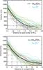 |
Fig. 9 Horizontal MF velocities, vMF(r), in m/s of 51 observed 3 h velocity maps against the distance from the spot center in spot ratio (upper panel) and the distance to the sunspot in Mm (lower panel). The calculated average (black bold curve) is drawn. |
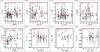 |
Fig. 10 Correlations of sunspot and MF properties for all 51 sunspot maps
(a)–e)), v3h, and their evolution within
one week for 20 sunspots (f)–h)) indicated by linear regressions (red
lines) and the coefficients, |

4.1. Horizontal moat flow velocity: vMF(r)
In the appendix, Figs. A.1 and A.2, we display the radial dependence of the horizontal flow component for all 51 sunspot maps. Since this is the first time that the EF and MF are analyzed coherently for more than only a few spots, it is very remarkable to find that all our spots behave very similarly. The radial dependence is qualitatively the same for all spots. At first glance, only the sunspot size and the maximum of the EF velocity vary. As described in Sect. 3.4 the kink between the velocity decrease of the EF in the penumbra (PU) and the MF at the spot boundary is recognizable for all sunspots in the radial dependences displayed in Figs. A.1 and A.2. In the next step, we examine the flow properties of all spots in detail and compare them.
The moat flow was identified for all selected sunspots as a predominantly horizontal,
axially symmetrical flow starting just outside of the penumbra with velocities depending
on the distance, r, to the sunspot. Figure 9 displays the strong decay of the MF velocities,
 for all
51 analyzed MF regions based on v3h. The upper panel shows the
decrease with respect to the distance from the spot center in the radius ratio,
for all
51 analyzed MF regions based on v3h. The upper panel shows the
decrease with respect to the distance from the spot center in the radius ratio,
 .
The lower panel plots the MF velocities against the distance,
.
The lower panel plots the MF velocities against the distance,
 , from the penumbral boundary.
The monotone decrease from maximum velocities of
vMF(r = 0) = 800...1200 m/s
just outside the sunspot is largely similar for all sunspots. The average run,
, from the penumbral boundary.
The monotone decrease from maximum velocities of
vMF(r = 0) = 800...1200 m/s
just outside the sunspot is largely similar for all sunspots. The average run,
 ,
starts with 1000 m/s just beyond the penumbral boundary at
r = 0 Mm and decreases to approx. 500 m/s within
r = 4 Mm or
,
starts with 1000 m/s just beyond the penumbral boundary at
r = 0 Mm and decreases to approx. 500 m/s within
r = 4 Mm or  . The average
velocity falls below the typical rms values,
σrms ≈ 180 m/s, at
r = 9.2 Mm or
. The average
velocity falls below the typical rms values,
σrms ≈ 180 m/s, at
r = 9.2 Mm or  . Consequently, the
MF velocity highly depends on the location within the MF region. We compare both panels of
Fig. 9 and notice that the runs according to the
radius ratio in the left hand panel are spread wider than according to the sheer distance
from the spot. Consequently, the MF appears to be independent of the spot size.
. Consequently, the
MF velocity highly depends on the location within the MF region. We compare both panels of
Fig. 9 and notice that the runs according to the
radius ratio in the left hand panel are spread wider than according to the sheer distance
from the spot. Consequently, the MF appears to be independent of the spot size.
This result is in line with recent studies describing the MF velocity on the surface ranging between vMF = 500...1000 m/s (Balthasar et al. 1996; Rimmele 1997; Vargas Domínguez et al. 2007), whereas the continuous velocity decrease with increasing distance from the spot boundary has not been measured before.
4.2. Maximum Evershed flow velocity: vEF
The maximum EF velocity, vEF = max [v∥ ,0 (RU ≤ r ≤ RS)], for all observed penumbrae is in the range of vEF = 1830...3000 m/s (Fig. 10e) with an average of 2325 m/s. Since we measure azimuthally averaged flow speeds of 3 h averages, our maximum EF velocities are slightly lower than the maximum velocities of up to 3...4 km s-1 found in recent studies (Schlichenmaier & Schmidt 2000; Shine et al. 1994; Rouppe van der Voort 2002; Bellot Rubio et al. 2003a). The location, rEF, of the extreme EF velocity can by found at 0.65 RS ≤ rEF ≤ 0.87 RS, with an average ratio of rEF = 0.78 RS which is not as far in the outer spot boundary as rEF = 0.8...0.9 RS (Tritschler et al. 2004; Franz 2011). The velocity run within the penumbra is largely similar for all sunspots with some differences in the skewness as seen in Figs. A.1 and A.2.
4.3. Correlations
In the following section, we analyze the correlations between vMF, aMF, vEF, and RS based on the 3 h average sample.
4.3.1. Correlation of spot size and MF velocity
In order to work out the interaction of the sunspots with their moat flows, we plot the
MF velocities,
vMF = ⟨ vMF(r) ⟩ r = 0,...,5px,
against the sunspot size, RS, as it can be seen in Fig.
10a with a nonsignificant rise of the linear
regression (red line) and a correlation coefficient of
 .
Hence, we find that the MF velocity is in average around 1000 m/s and does not depend on
the spot size. Since we measure close to the outer sunspot boundary the indicated slight
increase may be due to a stronger EF in bigger sunspots (see Sects. 4.3.3 and 4.3.4).
.
Hence, we find that the MF velocity is in average around 1000 m/s and does not depend on
the spot size. Since we measure close to the outer sunspot boundary the indicated slight
increase may be due to a stronger EF in bigger sunspots (see Sects. 4.3.3 and 4.3.4).
4.3.2. Correlation of spot size and MF extension
According to Eq. (7) the MF extensions,
aMF, were determined for all sunspots with a boundary
criteria of σrms ≈ 180 m/s and range
between aMF = 5...15 Mm for the spot
sizes of RS = 8.6...21.2 Mm, cf. Fig.
10b. Since the linear regression and the
correlation coefficient of  indicate uncorrelated components, we average the MF extensions to
⟨ aMF ⟩ 51 spots = 9.2 Mm. Comparing our
results to other studies (e.g., Brickhouse &
Labonte 1988) the MF extension lies below the mentioned
aMF = 10...20 Mm for small sunspots and
far below the double spot radius for larger spots. In our studies, the MF extension is
independent of the spot size and therefore is in the order of the sunspot size only for
small but not for bigger spots. This finding goes in line with studies by Sobotka & Roudier (2007). In summary it can
be stated that we find four indications that the MF is not correlated to the spot size:
(i) the kink of v∥ ,0(r)
at the outer spot boundary (e.g. Fig. 8: upper
panel), (ii) the smaller spread of all 51 MFs by merely displaying them with their
radial distance from the spot in Fig. 9, (iii) the
trend in Fig. 10a and (iv) the trend in Fig. 10b.
indicate uncorrelated components, we average the MF extensions to
⟨ aMF ⟩ 51 spots = 9.2 Mm. Comparing our
results to other studies (e.g., Brickhouse &
Labonte 1988) the MF extension lies below the mentioned
aMF = 10...20 Mm for small sunspots and
far below the double spot radius for larger spots. In our studies, the MF extension is
independent of the spot size and therefore is in the order of the sunspot size only for
small but not for bigger spots. This finding goes in line with studies by Sobotka & Roudier (2007). In summary it can
be stated that we find four indications that the MF is not correlated to the spot size:
(i) the kink of v∥ ,0(r)
at the outer spot boundary (e.g. Fig. 8: upper
panel), (ii) the smaller spread of all 51 MFs by merely displaying them with their
radial distance from the spot in Fig. 9, (iii) the
trend in Fig. 10a and (iv) the trend in Fig. 10b.
4.3.3. Correlation of spot size and EF velocity
To yield the correlation of the sunspot properties, i. e. the maximum horizontal EF
velocity between
vEF = 1830...3000 m/s
and the sunspot radius, we plot both components against each other in Fig. 10e and fit a linear regression by considering all
values. We obtain a slightly positive trend for bigger sunspots harboring higher maximum
EF velocities. Following the regression, sunspots with
RS = 10 Mm would have maximum EF velocities of 2200 m/s
whereas sunspots with the double size yield maximum EF velocities that are almost
500 m/s faster. Although there are some outliers between 16−17 Mm, even the correlation
coefficient,  ,
suggests a positive link of the EF velocity with the spot size.
,
suggests a positive link of the EF velocity with the spot size.
4.3.4. Correlation of Evershed flow and moat flow
As we pointed out in Sects. 4.3.1 and 4.3.2 the moat flow seems to be independent of the
sunspot radius. In the following, we examine the largely unknown link between the
penumbral EF and the adjacent MF. It is therefore important to find out whether higher
EF velocities also cause higher MF velocities or a bigger MF extension, which would
argue for a partial drive of the MF by the EF. Due to Figs. 10c–d which plot the MF velocities,
vMF, and MF extensions,
aMF, against the EF velocities,
vEF, with correlation coefficients of
 and
and  ,
we draw the conclusion that the EF has no impact on the MF. This means that there is a
greater decrease in speed for spots with higher maximum EF velocities toward the outer
penumbral boundary (see Figs. A.1 and A.2). Although the existence of the MF is directly
coupled to the existence of a penumbra and its EF, the observed properties indicate the
MF and the EF are independent sunspot flows.
,
we draw the conclusion that the EF has no impact on the MF. This means that there is a
greater decrease in speed for spots with higher maximum EF velocities toward the outer
penumbral boundary (see Figs. A.1 and A.2). Although the existence of the MF is directly
coupled to the existence of a penumbra and its EF, the observed properties indicate the
MF and the EF are independent sunspot flows.
4.4. Weekly evolution
To study the temporal evolution of the analyzed components, i.e. RS, vMF, aMF, and vEF, we have tracked 20 sunspots (see Table A.1) from the eastern to the western limb sides and performed the analysis of v3h for a second time at θ ≈ 50°. According to the latitude and the differential rotations, the observing dates range between 6 to 8 days.
The weekly changes are in the range of
ΔRS = −3...1 Mm,
ΔvEF = ±500 m/s,
ΔvMF = ±200 m/s and
ΔaMF = −8...3 Mm. Figures 10f–g plot the changes, ΔvMF
and ΔaMF, of the MF velocities and extensions against the
change of the spot radius, ΔRS, with linear regressions
according to the correlation coefficients,  and
and  ,
indicating slightly negative trends. Following this, the MF velocity increases for
strongly decaying sunspots and tends to decrease slightly for small
ΔRS. The MF extension, aMF,
decreases for the majority of the sunspots with some exceptions for strongly decaying
sunspots, but yields no significant correlation with the sunspot evolution. Figure 10h plots the change in the MF velocities,
ΔvMF, against the changing MF extension,
ΔaMF, with no significant correlation,
,
indicating slightly negative trends. Following this, the MF velocity increases for
strongly decaying sunspots and tends to decrease slightly for small
ΔRS. The MF extension, aMF,
decreases for the majority of the sunspots with some exceptions for strongly decaying
sunspots, but yields no significant correlation with the sunspot evolution. Figure 10h plots the change in the MF velocities,
ΔvMF, against the changing MF extension,
ΔaMF, with no significant correlation,
 .
Because they are
.
Because they are  ,
,
 ,
,
 ,
all other correlations are insignificant and yield no further impact. According to these
results, we would draw the conclusions, that a strong sunspot decay leads to an additional
drive of the moat flow by accelerating its velocity and sporadically expanding its
outreach, whereas it has no impact on the EF velocity.
,
all other correlations are insignificant and yield no further impact. According to these
results, we would draw the conclusions, that a strong sunspot decay leads to an additional
drive of the moat flow by accelerating its velocity and sporadically expanding its
outreach, whereas it has no impact on the EF velocity.
4.5. Monthly evolution
Tracking three long-lasting sunspots across the far side of the Sun, they reappear at the eastern front side (Table A.1: No. 4 → 6, 7 → 9,11 → 13; Figs. 6e–h). This allows us to study the long-term evolution for one month in order to crosscheck the results of the weekly evolution. The changes in sunspot size, ΔRS, the MF velocity, ΔvMF, the MF extension, ΔaMF, and the maximum EF velocity, ΔvEF, as listed in Table 1 are based on the mean difference between the first and second appearances.
Monthly evolution for three long-lasting sunspots.
Coupled to the strong decay in sunspot sizes, the MF velocity significantly increases, whereas the EF velocity shows a decrease of several hundred m/s. These trends are in line with the correlations for the weekly evolution. The size of the MF region shows no unique trend, but the huge widening ΔaMF = +6.6 Mm of Spot-No. 7 (in Table 1) by more than 6 Mm could underline an additional outflow of plasma over the moat cell due to a strong sunspot decay.
5. Conclusion
5.1. Conclusions on the moat flow
Meyer et al. (1979) suggested that a sunspot is embedded in a supergranular cell. If one puts MF cells in a context with supergranules, one should realize that they have a diameter between 30 and 60 Mm, i.e., are up to twice as large as supergranules. Also, the MF velocities are more than twice as high as supergranular velocities (e.g., Brickhouse & Labonte 1988). As a result, the MF needs a driving mechanism that is distinct from the driving mechanism of normal supergranules. Nye et al. (1988) modeled the MF being driven by a surplus gas pressure beneath the penumbra, arguing that the lack of radiative cooling beneath the penumbra generates a surplus of heat, hence gas pressure. In these models the MF velocity depends on the depth of the penumbra, but not on the size of a spot. At that time this posed a problem, as it was commonly believed that the MF extension scales with the spot radius. Later, Sobotka & Roudier (2007) provided evidence that there is no correlation between the MF and the spot radius. Our investigation based on Doppler shift measurements rather than on local correlation tracking, independently confirms these later findings. The evidence therefore supports the moat flow model in which the driving forces are due to surplus gas pressure beneath sunspots.
A moat flow that is driven from beneath the penumbra would naturally push away the granules from the spot as seen with local correlation techniques. This implies that the MF is present in the deep photosphere. In contrast, the Evershed flow or the fraction of it that extends from the penumbra outwards into the moat is present in the magnetic canopy that surrounds the sunspot in the mid and upper photosphere (Rezaei et al. 2006). In the immediate surroundings of the sunspot two types of flows exist: (1) the (magnetic) EF that partially continues in the magnetic canopy, which ascends outwards from the mid-photosphere at the spot boundary; (2) the (largely nonmagnetic) MF in the deep photosphere and beneath.
We consider the MMFs to be distinct from the moat flow. They migrate into or are advected by the MF. MMFs are associated with inclined magnetic field lines (relative to horizontal) that reach up into the higher atmospheric layers. These MMF field lines possibly originate in the sunspot and either witness the decay of sunspots (uni-polar MMFs) or are due to some waves that propagate outwards (bipolar MMFs), (see e.g., Sainz Dalda & Martínez Pillet 2005; Sainz Dalda & Bellot Rubio 2008a,b; Schlichenmaier 2002). Because of their vertical configuration, outwardly migrating MMFs can also be detected in higher atmospheric layers as reported by Sobotka & Roudier (2007).
5.2. Summary
We calibrated HMI velocity maps such that systematic absolute errors are below 150 m/s on an absolute scale. The synoptic CLV of the convective blueshift was measured in good accordance with previous findings and the theoretical synthesis curve. We find a maximum velocity of the solar rotation of 1992 m/s, which agrees with previous measurements and reveals no significant impact by stray light. The instrumental artifacts were identified in line with HMI calibration studies (Centeno et al. 2011). These artifacts make the meridional flow amplitude too small to be measured.
We analyzed 3 h time averages of sunspot flow velocities. We constructed 51 velocity maps of 31 sunspots. The flow in and around circular sunspots with a fully developed penumbra was analyzed using azimuthal averages, thereby assuming axial symmetry. In both, the MF and EF, the horizontal velocity component was dominant. The vertical flow components of MF and EF were determined to be small. Since the exact amount of convective blueshift is unknown, we do not address the sign of vertical flows.
The radial dependence of the velocity fields was observed to be similar for all 51 sunspot maps. The analysis of the EF yielded results that are consistent with recent studies. A higher EF velocity was detected for bigger sunspots, and the EF velocity scales with the spot size. The MF is a convective outflow with radially decreasing velocity. The MF velocity turned out to be similar in size and independently of the spot size. Also, the MF extension is not correlated with any sunspot property. As MF and EF properties turn out to be uncorrelated, we inferred that the driving mechanisms of the two flows should be distinct. Therefore, we favor the MF model of Nye et al. (1988): the MF is driven by surplus gas pressure beneath the penumbra.
We find a tendency toward increasing MF velocity for strongly decaying sunspots on time scales of one week (spot rotates from the east to west limbs) and one month (spot reappears on the east limb). It is beyond the scope of this paper to put this into the context of a model for decaying sunspots.
Online material
Appendix A: Analyzed sunspots
List of the 31 numbered, observed sunspots.
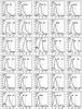 |
Fig. A.1 Horizontal flow velocities, v∥ ,0(r), in km s-1 from the sunspot center (r = 0 Mm) to a distance of 36 Mm in the quiet Sun(QS) for spots No. 1–17 (see Table A.1). The boundaries of the umbra (U), the penumbra (PU), and the end of the moat flow region (MF) are indicated as vertical dashed lines. |
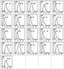 |
Fig. A.2 Horizontal flow velocities, v∥ ,0(r), in km s-1 from the sunspot center (r = 0 Mm) to a distance of 36 Mm in the quiet Sun(QS) for spots No. 18–31 (see Table A.1). The boundaries of the umbra (U), the penumbra (PU), and the end of the moat flow region (MF) are indicated as vertical dashed lines. |
A velocity map of the Sun according to spectral line shifts due to the Doppler effect.
Keywords for observer motion in the FITS file header: OBS_VR (radial), OBS_VW (westward), and OBS_VN (northward).
A large-scale axisymmetrical flow directing from the equator to the poles on the solar surface with velocities up to 20 m/s at latitudes around 35° (Hathaway & Rightmire 2010; Komm et al. 2011).
Zürich Classification: Group H.
Acknowledgments
The HMI instrument of NASA’s SDO mission is operated by the HMI/AIA Joint Science Operations Center (JSOC) at Stanford University. The data was provided by the JSOC webpage. We want to thank H.-G. Ludwig for the spectral line synthesis, R. Centeno and S. Couvidat for their correspondence on HMI questions, and J. M. Borrero for his fruitful comments on the manuscript.
References
- Balthasar, H. 1985, Sol. Phys., 99, 31 [NASA ADS] [CrossRef] [Google Scholar]
- Balthasar, H., & Muglach, K. 2010, A&A, 511, A67 [NASA ADS] [CrossRef] [EDP Sciences] [Google Scholar]
- Balthasar, H., Schleicher, H., Bendlin, C., & Volkmer, R. 1996, A&A, 315, 603 [NASA ADS] [Google Scholar]
- Beeck, B., Collet, R., Steffen, M., et al. 2012, A&A, 539, A121 [NASA ADS] [CrossRef] [EDP Sciences] [Google Scholar]
- Brickhouse, N. S., & Labonte, B. J. 1988, Sol. Phys., 115, 43 [NASA ADS] [CrossRef] [Google Scholar]
- Bellot Rubio, L. R., Balthasar, H., Collados, M., & Schlichenmaier, R. 2003a, A&A, 403, 47 [Google Scholar]
- Cabrera Solana, D., Bellot Rubio, L. R., Beck, C., & del Toro Iniesta, J. C. 2006, ApJ, 649, L41 [NASA ADS] [CrossRef] [Google Scholar]
- Cabrera Solana, D., Bellot Rubio, L. R., Beck, C., & del ToroIniesta, J. C. 2007, A&A, 475, 1067 [NASA ADS] [CrossRef] [EDP Sciences] [Google Scholar]
- Centeno, R., Tomczyk, S., Borrero, J. M., et al. 2011, Proc. Sol. Polarisation Workshop 6, 437, 147 [NASA ADS] [Google Scholar]
- Cruz Rodríguez, J., de La Kiselman, D., & Carlsson, M. 2011, A&A, 528, A113 [NASA ADS] [CrossRef] [EDP Sciences] [Google Scholar]
- Delbouille, L., Roland, G., & Neven, L. 1990, Atlas photometrique DU spectre solaire, Université de Liège [Google Scholar]
- Evershed, J. 1909, MNRAS, 69, 454 [NASA ADS] [CrossRef] [Google Scholar]
- Featherstone, N. A., Hindman, B. W., & Thompson, M. J. 2011, J. Phys.: Conf. Ser., 271, 012002 [NASA ADS] [CrossRef] [Google Scholar]
- Franz, M. 2011, Spectropolarimetry of Sunspot Penumbrae, Cuvillier Göttingen [Google Scholar]
- Franz, M., & Schlichenmaier, R. 2009, A&A, 508, 1453 [NASA ADS] [CrossRef] [EDP Sciences] [Google Scholar]
- Freytag, B., Steffen, M., Ludwig, H.-G., et al. 2012, J. Comp. Phys., 231, 919 [Google Scholar]
- Gizon, L., Duvall, T. L., Jr., & Larsen, R. M. 2000, JA&A, 21, 339 [NASA ADS] [CrossRef] [Google Scholar]
- Gizon, L., Schunker, H., Baldner, C. S., et al. 2009, Space Sci. Rev., 144, 249 [NASA ADS] [CrossRef] [Google Scholar]
- Harvey, K., & Harvey, J. 1973, Sol. Phys., 28, 61 [NASA ADS] [CrossRef] [Google Scholar]
- Hathaway, D., & Rightmire, L. 2010, Science, 327, 1350 [NASA ADS] [CrossRef] [Google Scholar]
- Howe, R., Jain, K., Hill, F., et al. 2011, J. Phys.: Conf. Ser., 271, 012060 [Google Scholar]
- Komm, R., Howe, R., Hill, F., et al. 2011, J. Phys.: Conf. Ser., 271, 012077 [NASA ADS] [CrossRef] [Google Scholar]
- Maltby, P. 1964, Astrophys. Norvegica, 8, 205 [Google Scholar]
- Meyer, F., Schmidt, H. U., & Weiss, N. O. 1979, A&A, 76, 35 [NASA ADS] [Google Scholar]
- Michard, R. 1951, Ann. Astrophys., 14, 101 [NASA ADS] [Google Scholar]
- Nye, A., Bruning, D., & LaBonte, B. J. 1988, Sol. Phys., 115, 251 [NASA ADS] [CrossRef] [Google Scholar]
- Pardon, L., Worden, S. P., & Schneeberger, T. J. 1979, Sol. Phys., 63, 247 [NASA ADS] [CrossRef] [Google Scholar]
- Rezaei, R., Schlichenmaier, R., Beck, C., & Bellot Rubio, L. R. 2006, A&A, 454, 975 [NASA ADS] [CrossRef] [EDP Sciences] [Google Scholar]
- Rimmele, T. R. 1994, A&A, 290, 972 [NASA ADS] [Google Scholar]
- Rimmele, T. R. 1997, ApJ, 490, 458 [NASA ADS] [CrossRef] [Google Scholar]
- Rouppe van der Voort, L. H. M. 2002, A&A, 389, 1020 [NASA ADS] [CrossRef] [EDP Sciences] [Google Scholar]
- Sainz Dalda, A., & Bellot Rubio, L. R. 2008a, A&A, 481, L21 [NASA ADS] [CrossRef] [EDP Sciences] [Google Scholar]
- Sainz Dalda, A., & Bellot Rubio, L. R. 2008b, A&A, 481, L21 [NASA ADS] [CrossRef] [EDP Sciences] [Google Scholar]
- Sainz Dalda, A., & Martínez Pillet, V. 2005, ApJ, 632, 1176 [NASA ADS] [CrossRef] [Google Scholar]
- Schlichenmaier, R. 2002, Astron. Nachr., 323, 303 [NASA ADS] [CrossRef] [Google Scholar]
- Schlichenmaier, R., & Collados, M. 2002, A&A, 381, 668 [NASA ADS] [CrossRef] [EDP Sciences] [Google Scholar]
- Schlichenmaier, R., & Schmidt, W. 1999, A&A, 349, L37 [NASA ADS] [Google Scholar]
- Schlichenmaier, R., & Schmidt, W. 2000, A&A, 358, 1122 [NASA ADS] [Google Scholar]
- Schlichenmaier, R., Bellot Rubio, L. R., & Tritschler, A. 2004, A&A, 415, 731 [NASA ADS] [CrossRef] [EDP Sciences] [Google Scholar]
- Schlichenmaier, R., Rezaei, R., Bello González, N., & Waldmann, T. A. 2010, A&A, 512, L1 [NASA ADS] [CrossRef] [EDP Sciences] [Google Scholar]
- Sheeley, N. R. Jr. 1969, Sol. Phys., 9, 347 [NASA ADS] [CrossRef] [Google Scholar]
- Sheeley, N. R. Jr. 1972, Sol. Phys., 25, 98 [NASA ADS] [CrossRef] [Google Scholar]
- Shine, R. A., Title, A. M., Tarbell, T. D., et al. 1994, ApJ, 430, 413 [NASA ADS] [CrossRef] [Google Scholar]
- Snodgrass, H. B. 1984, Sol. Phys., 94, 13 [NASA ADS] [CrossRef] [Google Scholar]
- Sobotka, M., & Roudier, T. 2007, A&A, 472, 277 [NASA ADS] [CrossRef] [EDP Sciences] [Google Scholar]
- Sobotka, M., Vázquez, M., Bonet, J. A., Hanslmeier, A., & Hirzberger, J. 1999, ApJ, 511, 436 [NASA ADS] [CrossRef] [Google Scholar]
- Solanki, S. K. 2003, A&ARv, 11, 153 [Google Scholar]
- Stix, M. 2002, The Sun (Berlin: Springer) [Google Scholar]
- Sun, M. T., Chou, D. Y., Lin, C. H., & the TON Team 1997, Sol. Phys., 176, 59 [NASA ADS] [CrossRef] [Google Scholar]
- Tritschler, A., Schlichenmaier, R., Bellot Rubio, L. R., et al. 2004, A&A, 415, 717 [NASA ADS] [CrossRef] [EDP Sciences] [Google Scholar]
- Vargas Domínguez, S., Bonet, J. A., Martínez Pillet, V., et al. 2007, ApJ, 660, L165 [NASA ADS] [CrossRef] [Google Scholar]
- Verma, M., Balthasar, H., Deng, N., et al. 2012, A&A, 538, A109 [NASA ADS] [CrossRef] [EDP Sciences] [Google Scholar]
- Vrabec, D. 1971, in Solar Magnetic Fields, ed. R. Howard, IAU Symp., 43, 329 [Google Scholar]
- Vrabec, D. 1974, in Chromospheric Fine Structure, ed. R. G. Athay (Dordrecht: Reidel), IAU Symp., 56, 201 [Google Scholar]
- Wiehr, E., & Degenhardt, D. 1992, A&A, 259, 313 [NASA ADS] [Google Scholar]
All Tables
All Figures
|
Fig. 1 Left panel: averaged velocity map, ⟨ v(x,y) ⟩ t = 61 days, with maximum blueshifts (eastern limb) and redshifts (western limb) with some 2 km s-1. The axes are given in arcsec. Right panel: reduced velocity map, ⟨ v(x,y) ⟩ t − vclv. |
| In the text | |
|
Fig. 2 a) Average CLV,
⟨ v(0,y) ⟩ t,
along the meridional centerline with an 8th-order polynomial fit,
vclv(y) (red curve) in m/s against
the distance y to the disk center in arcsec. b)
Calibrated, radially symmetrical CLV model,
vclv(r), with axis given in arcsec.
c) Convective blueshift,
vb(r), in
|
| In the text | |
|
Fig. 3 Absolute rotation velocities, vrot(l,B0 = 0), in m/s (black curve) on the solar surface for latitudes up to l = ±80° fitted by Ω(l) (red curve) and an equatorial maximum of Ω(0) = 1992 m/s. |
| In the text | |
|
Fig. 4 Computed differential rotation maps, vrot(d,l,B0 = 0°) (left panel) and vrot(d,l,B0 = 7.27°) (right panel), with maximum velocities vrot(l = 0,B0 = 0°) = 1992 m/s and vrot(l = 0,B0 = 7.27°) = 1976 m/s, spatially displayed in arcsec. |
| In the text | |
|
Fig. 5 Residual velocity map, vres(x,y), with axis given in arcsec. |
| In the text | |
|
Fig. 6 a) 720 s intensity map and b) corresponding 720 s
velocity map, |
| In the text | |
|
Fig. 7 Angular LOS velocities, vLOS(r,φ),
in m/s along the elliptical projection for θ = 51° of
circles with radius r = RS + 5 px
(left panel) and
r = RS + 10 px (right
panel) fitted by a sine curve (green, solid line) according to Eq.
(5). The amplitude,
|
| In the text | |
|
Fig. 8 Upper panel: horizontal flow velocities,
v∥ ,0(r), in m/s
for the distance, r, from the spot center in Mm. Error bars
represent the standard deviation. Dashed vertical lines mark the boundaries
between umbra (U), penumbra (PU), and moat flow region (MF) and the quiet Sun
(QS). Lower panel: horizontal LOS velocity,
|
| In the text | |
|
Fig. 9 Horizontal MF velocities, vMF(r), in m/s of 51 observed 3 h velocity maps against the distance from the spot center in spot ratio (upper panel) and the distance to the sunspot in Mm (lower panel). The calculated average (black bold curve) is drawn. |
| In the text | |
|
Fig. 10 Correlations of sunspot and MF properties for all 51 sunspot maps
(a)–e)), v3h, and their evolution within
one week for 20 sunspots (f)–h)) indicated by linear regressions (red
lines) and the coefficients, |
| In the text | |
|
Fig. A.1 Horizontal flow velocities, v∥ ,0(r), in km s-1 from the sunspot center (r = 0 Mm) to a distance of 36 Mm in the quiet Sun(QS) for spots No. 1–17 (see Table A.1). The boundaries of the umbra (U), the penumbra (PU), and the end of the moat flow region (MF) are indicated as vertical dashed lines. |
| In the text | |
|
Fig. A.2 Horizontal flow velocities, v∥ ,0(r), in km s-1 from the sunspot center (r = 0 Mm) to a distance of 36 Mm in the quiet Sun(QS) for spots No. 18–31 (see Table A.1). The boundaries of the umbra (U), the penumbra (PU), and the end of the moat flow region (MF) are indicated as vertical dashed lines. |
| In the text | |
Current usage metrics show cumulative count of Article Views (full-text article views including HTML views, PDF and ePub downloads, according to the available data) and Abstracts Views on Vision4Press platform.
Data correspond to usage on the plateform after 2015. The current usage metrics is available 48-96 hours after online publication and is updated daily on week days.
Initial download of the metrics may take a while.