| Issue |
A&A
Volume 551, March 2013
|
|
|---|---|---|
| Article Number | A82 | |
| Number of page(s) | 11 | |
| Section | Extragalactic astronomy | |
| DOI | https://doi.org/10.1051/0004-6361/201220428 | |
| Published online | 27 February 2013 | |
No temperature fluctuations in the giant H II region H 1013
1
LUTH, Observatoire de Paris, CNRS, Université Paris Diderot,
Place Jules Janssen,
92190
Meudon,
France
e-mail: This email address is being protected from spambots. You need JavaScript enabled to view it.
2
Instituto de Astronomía, Universidad Nacional Autónoma de
México, Apdo. Postal 70264, Méx.
D.F., 04510
Mexico,
Mexico
e-mail: This email address is being protected from spambots. You need JavaScript enabled to view it.
3
Instituto de Astrofísica de Canarias, 38200, La Laguna, Tenerife, Spain
e-mail: This email address is being protected from spambots. You need JavaScript enabled to view it.
4
Departamento de Astrofísica, Universidad de La
Laguna, 38205, La
Laguna, Tenerife,
Spain
5
Institute for Astronomy, 2680 Woodlawn Drive, Honolulu, HI
96822,
USA
e-mail: This email address is being protected from spambots. You need JavaScript enabled to view it.
6
Geneva Observatory, University of Geneva,
51 Ch. des Maillettes,
1290
Versoix,
Switzerland
7
CNRS, IRAP, 14
avenue E. Belin, 31400
Toulouse,
France
8
Leiden Observatory, Leiden University,
PO Box 9513, 2300 RA
Leiden, The
Netherlands
Received: 21 September 2012
Accepted: 18 January 2013
Abstract
While collisionally excited lines in H ii regions allow one to easily probe the chemical composition of the interstellar medium in galaxies, the possible presence of important temperature fluctuations casts some doubt on the derived abundances. To provide new insights into this question, we have carried out a detailed study of a giant H ii region, H 1013, located in the galaxy M101, for which many observational data exist and which has been claimed to harbour temperature fluctuations at a level of t2 = 0.03−0.06. We have first complemented the already available optical observational datasets with a mid-infrared spectrum obtained with the Spitzer Space Telescope. Combined with optical data, this spectrum provides unprecedented information on the temperature structure of this giant H ii region. A preliminary analysis based on empirical temperature diagnostics suggests that temperature fluctuations should be quite weak. However, only a detailed photoionization analysis taking into account the geometry of the object and observing apertures can make a correct use of all the observational data. We have performed such a study using the pyCloudy package based on the photoionization code Cloudy. We have been able to produce photoionization models constrained by the observed Hβ surface brightness distribution and by the known properties of the ionizing stellar population than can account for most of the line ratios within their uncertainties. Since the observational constraints are both strong and numerous, this argues against the presence of significant temperature fluctuations in H 1013. The oxygen abundance of our best model is 12 + log O/H = 8.57, as opposed to the values of 8.73 and 8.93 advocated by Esteban et al. (2009, ApJ, 700, 654) and Bresolin (2007, ApJ, 656, 186), respectively, based on the significant temperature fluctuations they derived. However, our model is not able to reproduce the intensities of the oxygen recombination lines observed by Esteban et al., as well as the very low Balmer jump temperature inferred by Bresolin. We have argued that the latter might be in error, due to observational difficulties. On the other hand, the discrepancy between model and observation as regards the recombination lines cannot be attributed to observational uncertainties and requires an explanation other than temperature fluctuations.
Key words: ISM: abundances / HII regions / galaxies: individual: H 1013
© ESO, 2013
1. Introduction
Giant H ii regions are among the most effective probes of the chemical composition of the present-day interstellar medium in galaxies. Methods to derive abundances in these objects have been devised many years ago (Aller & Menzel 1945) and are straightforward. If the electron temperature can be measured using a temperature indicator such as the emission line ratio [O iii] λ4363/5007 or [N ii] λ5755/6584, the ionic abundances can be obtained directly from the intensities of lines emitted by the ions. Elemental abundances are then obtained by correcting for unseen ionic stages, as explained e.g. in Osterbrock (1989) or Stasińska (2004).
There are, however, a few issues which have appeared over the years for which no broadly accepted solution yet exists and which cast some doubts on the derived abundances. One of them is the question of the possible presence of important “temperature fluctuations” in H ii regions (which should better be called “temperature inhomogeneities”). It has been argued by Peimbert (1967) that such fluctuations are likely to exist, since the temperature derived from the observed Balmer jump is significantly lower than that derived from [O iii] λ4363/5007. Peimbert & Costero (1969) showed that such temperature fluctuations would bias the derived abundances with respect to hydrogen towards values that are systematically too low, unless one adopts their proposed temperature fluctuation scheme to account for them. However, up to now, no mechanism has been found to produce temperature fluctuations to a level of t2 ~ 0.04 which is a typical value proposed by Peimbert & coworkers (Peimbert 1967; Peimbert & Peimbert 2011). It is, however, possible that several mechanisms proposed by various authors (e.g. such as those summarized by Torres-Peimbert & Peimbert 2003) may add up to produce the observed level of temperature fluctuations. Another, perhaps related question, is that ionic abundances derived from recombination lines are systematically higher than those derived from optical collisionally excited lines (see e.g. García-Rojas & Esteban 2007, for a review and a general discussion). These discrepancies could be due to the same temperature inhomogeneities that explain the difference between the temperatures derived from the Balmer jump and the temperatures derived from [O iii] λ4363/5007. In that case, it is believed that abundances obtained from recombination lines are the correct ones, since recombination lines have roughly the same – weak – temperature dependence, while optical collisionally excited lines have a very strong temperature dependence and are thus affected by temperature inhomogeneities (see e.g. Stasińska 2009). Other interpretations of these abundance discrepancies are also possible, such as abundance inhomogeneities (Tsamis & Péquignot 2005; Stasińska et al. 2007), density inhomogeneities (Mesa-Delgado et al. 2012), departure from a Maxwellian energy distribution of the electrons (Nicholls et al. 2012), or simply inaccurate theoretical rates for the recombination coefficients (Pradhan et al. 2011). Finally, as shown by Stasińska (2005), even in the absence of abundance or density inhomogeneities, a further issue is represented by the fact that metal-rich H ii regions do not appear as such when using classical temperature-based abundance determinations from optical lines, due to an important internal temperature gradient caused by strong emission of infrared lines in the central zones.
In this paper, we perform a detailed analysis of the extragalactic H ii region H 1013 in the spiral galaxy M 101, in order to look for some clues to the problem enunciated above. H 1013 is a giant H ii region, for which deep spectra have recently been obtained on very large telescopes (Bresolin 2007; Esteban et al. 2009). The oxygen abundances derived by these authors from optical collisionally excited lines, without accounting for temperature fluctuations, are 12 + log (O/H) = 8.52 and 8.45, respectively. The abundance of O++ derived by Esteban et al. (2009) from recombination lines is larger than that derived from [O iii] λ5007 by a factor of 2.5. From this discrepancy, and attributing it to temperature fluctuations, these authors find t2 = 0.037 ± 0.020. They also obtain an estimate of t2 using a maximum likelihood method from various helium line intensities and obtained t2 = 0.031 ± 0.017. On the other hand, from his estimate of the Balmer jump temperature, TBJ = 5000 ± 800 K, and of the temperature deduced from the [O iii] λ4363/5007 line ratio, T[O iii] = 7700 ± 250 K, Bresolin (2007) obtains a temperature fluctuation factor t2 = 0.06 ± 0.02, which implies an oxygen abundance larger by about a factor of 4 using the Peimbert & Costero (1969) scheme. H 1013 is thus an object where previous studies argued for the presence of important temperature inhomogeneities. In order to acquire additional constraints, we obtained mid-infrared spectroscopic observations with the Spitzer Space Telescope. Mid-infrared lines are crucial in the diagnostic of the physical conditions of this object, since their emissivities depend very little on the electron temperature. In addition, they allow one to resolve the above-mentioned degeneracy in abundance determinations. In order to make the best use of this new information, we construct a photoionization model of H 1013 that is as realistic as possible and constrained by all the available data, including the size and positions of the observing apertures.
The organization of the paper is as follows. In Sect. 2 we present the observational data used in this study. In Sect. 3 we deduce from them some properties of the ionizing radiation field and of the gas density distributions that will be used as an input in the photoionization modeling. In Sect. 4 we describe our photoionization modeling procedure. In Sect. 5, we present our results. A brief summary and general conclusions are presented in Sect. 6.
2. Observational dataset
2.1. Narrow-band filter images
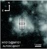 |
Fig. 1 Portion of the Hα continuum-subtracted image of M 101 presented by Cedrés & Cepa (2002) showing the H ii region H 1013. The apertures corresponding to the optical and infrared spectra used in this study are also indicated for reference: the long narrow one corresponds to the LRIS data, the short narrow one to the HIRES data, and the wide one to the mid-infrared observations (note that the slit orientation is arbitrary). |
Cedrés & Cepa (2002) used CDD observations in several narrow-band filters to compile a catalogue of 338 H ii regions in the inner parts of M 101 (NGC 5457), also providing information about their fluxes, extinctions, equivalent widths, spatial distribution, excitations, radiation hardness, ionization parameters and metallicities. H 1013 is identified as the H ii region number 299 in their catalogue.
We use the Hα and Hβ continuum-subtracted images (kindly provided by B. Cedrés) in our study. These images were obtained at the Nordic Optical Telescope with the ALFOSC instrument in direct imaging mode (spatial resolution of 0.189 arcsec/pix). A description of the reduction process (also including flux calibration and adjacent continuum subtraction) can be found in the original paper by Cedrés & Cepa. Images through additional narrow-band filters (Hβ, [O ii], [O iii], [S ii] and [S iii]) are also available, however the error bars on the integrated line ratios are too large (>50%) to provide useful constraints to our models.
Figure 1 presents a small portion of the original continuum-subtracted Hα image, centered on H 1013. The size and location of the apertures used to obtain the optical and infrared spectra described in Sects. 2.2 and 2.3 are also indicated for reference. As can be noticed, the three apertures cover different portions of the H ii region, and none covers the whole region. This is an important point that must be taken into account when comparing the results of our photoionization model with the various spectroscopic observations (or when combining optical with mid-infrared lines).
The continuum-subtracted Hβ image is used in Sect. 3.3 to obtain the nebular density profile. In Sect. 3.1 we also use the total extinction-corrected Hβ flux provided by Cedrés & Cepa to constrain the properties of the ionizing stellar population of H 1013.
2.2. Optical spectra
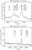 |
Fig. 2 The WR features in the optical spectrum of Bresolin (2007). |
Two sets of optical spectra are available. The first one is from Bresolin (2007), and was obtained with the Low Resolution Imaging Spectrometer (LRIS) spectrograph at the Keck I telescope. The slit size was 1.5 arcsec × 14 arcsec. The seeing during the observations was 0.7 arcsec. Three spectra were taken: a blue spectrum: 3300–5600 Å (FWHM spectral resolution ~5 Å); red spectrum: 4960–6670 Å (spectral resolution ~4 Å); near-infrared spectrum: 6050–9800 Å (spectral resolution ~9 Å). We adopt the dereddened line intensities from Bresolin (2007).
The second spectrum we consider is that by Esteban et al. (2009). It was taken with the High Resolution Echelle Spectrometer (HIRES) at the Keck I telescope. The spectrum covers the 3550–7440 Å region with a spectral resolution of 23 000. The slit width was 1.5 arcsec and the extraction was performed over the central 5.76 arcsec. The dereddening procedure was slightly different from that adopted by Bresolin (2007) but, again, we adopted the dereddened line intensities from the original paper. The extraction apertures are indicated in Fig. 1 for both spectra (note that their orientation is arbitrary).
As a quick reference, the reddening-corrected line intensities with respect to Hβ are reported in the third column of Table 3, the label in Col. 2 indicating whether the data are from Bresolin (2007: B07) or Esteban et al. (2009: E09). The intensities of interest from the two sets of observations agree in general very well within the quoted error bars. A notable exception is the case of [O ii] 3727+1, whose intensity from Esteban et al. (2009) is 40% smaller relative to the one obtained by Bresolin (2007). Such a large difference is not expected. Since the nearby high-order Balmer lines in Esteban et al. (2009) deviate from the recombination values by over two sigmas, we prefer to use the total [O ii] 3727+ intensity from Bresolin (2007) to constrain the photoionization models. However, we consider it safe to use the [O ii] λ3726/3729 line ratio from Esteban et al. (2009) to obtain an additional density diagnostic. Some other lines (e.g. [S ii] and [N ii]) have intensities that differ by more than the assigned error bars. This, a priori, can be due to the fact that the observing apertures are not the same.
2.3. Infrared spectrum
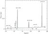 |
Fig. 3 Spitzer Space Telescope spectrum of H 1013. |
Spitzer spectrum line measurements (Slit: 11.3 × 4.7 arcsec2).
A mid-infrared (mid-IR) spectrum of H 1013 was obtained with the Infrared Spectrograph (IRS, Houck et al. 2004) aboard the Spitzer Space Telescope on 26 April 2007 (program ID 30205). The Short-High module was used to cover the 9.9–19.6 μm wavelength range with a 11.3 × 4.7 arcsec2 aperture and a spectral resolution R ≃ 600. We acquired 13 122 s cycles in IRS staring mode at two nod positions along the slit. The total integration time was 53 min. The pipeline data were processed with IRSCLEAN (version 1.9) to create bad pixels masks, and with the SPICE GUI software (version 2.0.2) for spectral extraction. Since the spectra obtained from the two nod positions agree within the statistical noise, we combined them to yield the final, flux-calibrated spectrum of H 1013, shown in Fig. 3. The fluxes of the emission lines present in the spectrum were measured with the splot task within IRAF2, and are summarized in Table 1, both in terms of absolute flux (in erg cm-2 s-1) and relative to the H I 7–6 line. In principle, the absolute calibration of the mid-IR data is correct within 30%, but we prefer to use the mid-IR and optical hydrogen lines to rescale the mid-IR spectrum (see later). This ensures that line flux ratios are correct across the whole wavelength range.
3. Derivation of stellar and nebular properties
3.1. The ionizing stellar population
The first thing to note is that the spectrum of H 1013 contains Wolf-Rayet (WR) features (see Fig. 2). This means that, if the ionizing cluster can be approximated by an instantaneous starburst of large enough mass, its age is around 2–5 Myr.
To obtain the total number of ionizing photons, we assume in the first place that all the stellar ionizing photons are absorbed by the nebular gas. We adopt a distance to M 101 of 7 Mpc (a compromise between the value of 7.5 Mpc from Sandage & Tammann 1976 and that of 6.85 Mpc from Freedman et al. 2001). From a total extinction-corrected flux in Hβ of 3.6 ± 1.2 × 10⁻¹³ erg cm-2 s-1 (Cedrés & Cepa 2002), we obtain a total number of hydrogen ionizing photons QH = 4.42 × 1051 s-1. Adopting a Kroupa (2001) stellar initial mass function and using the Starburst99 stellar synthesis code (Leitherer et al. 1999) to relate stellar masses, ages and ionizing photon output, we find that, for an age of 2.5 Myr (appropriate for our object, as will be shown below), this corresponds to a total of ~1.3 × 10⁵ M⊙ of stars with initial masses between 0.1 and 100 M⊙. In fact, dust must be present inside the H ii region, since iron is heavily depleted (Esteban et al. 2009), and therefore absorbs part of the ionizing photons. In our final models (see below), dust absorbs about 1.5 × 1051 ph s-1, therefore the total initial stellar mass of the ionizing cluster is about ~1.7 × 10⁵ M⊙. According to Cerviño et al. (2003), the minimum initial cluster mass necessary to derive trustworthy results from photoionization models at an age of about 2.5 Myr is at least 105 M⊙ for the ions we are interested in, if using classical synthesis models that assume full sampling of the initial mass function. Those authors however recommend a value 30 times larger for really safe results. Clearly, our object does not comply with such conditions. In the absence of direct information on the ionizing stars (such as is sometimes available, see Jamet et al. 2004), a Monte-Carlo approach would in principle be needed. However, since the hardness of the ionizing radiation field is directly linked with the observed WR features, we may use the stellar population synthesis code Starburst99 to estimate the spectral energy distribution that produces the WR features observed in H 1013.
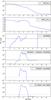 |
Fig. 4 Time dependence of several characteristics of an instantaneous starburst of solar metallicity obtained with Starburst99 (see text for details). The observed values or their upper limits in H 1013 are shown respectively by green and magenta horizontal lines. |
Figure 4 shows the time dependence of several features obtained by running Starburst99 with the expanding non-LTE stellar atmosphere models implemented by Smith et al. (2002), using the Geneva tracks and high mass-loss rates. The run of Starburst99 was made for solar metallicity, which is the most appropriate for our object. From top to bottom, Fig. 4 shows the values of
-
1.
EW(Hα), the equivalent width of the Hα emissionfor an instantaneous burst;
-
2.
the ratio QHe/QH of helium to hydrogen ionizing photons predicted by the model;
-
3.
the intensity of the stellar He ii λ4686 feature (2.5 × 10⁻¹⁵ erg cm-2 s-1);
-
4.
the intensity of the stellar N iii λ4640 + C iii λ4650 feature with respect to He ii λ4686;
-
5.
the intensity of the stellar C iii λ5696 feature with respect to He ii λ4686;
-
6.
and the intensity of the stellar C iv λ5808 feature with respect to He ii λ4686.
The observed values are represented with the green horizontal lines, the error bars with red dotted lines, and the upper limits (for C iii λ5696 and C iv λ5808) are represented with magenta lines. The QHe/QH ratio is actually not observed, but this value determines the observed value of the emission line ratio [O iii] λ5007/[O ii] λ3727 in the nebula. From Fig. 4, we see that the observed equivalent width of the Hα line indicates an age of 2–3 Myr, the intensity of the stellar He ii λ4686 feature is compatible with ages of about 2.5, 3.2 and 4.2 Myr, while the N iii λ4640 + C iii λ4650 feature indicates an age of 2.5–3 Myr, or larger than 5 Myr. On the other hand, the absence of observed stellar carbon features indicates an age smaller than 3 Myr. In fact, in the framework of an instantaneous starburst, the observational constraints on the stellar population are almost incompatible, but taking into account uncertainties, they point to an age of 2.5 Myr. However, if we consider that, in practice, a starburst is never instantaneous but occurs during a time interval of a few 105 yr, the range of possible solutions is larger. We approximate such a situation by considering two instantaneous starbursts of different intensities separated by a small time interval. After trials and errors, we find that combining one burst giving QH = 4.6 × 1051 ph s-1 at an age of 2.5 × 10⁶ yr and another one giving QH = 1 × 1050 ph s-1 at an age of 3 × 10⁶ yr correctly reproduces the observational constraints on the stellar population3 and allows us to correctly reproduce the observed emission line ratios of the nebula (see below).
3.2. Simple plasma diagnostics
Before proceeding to the description of the photoionization modeling, it is useful to consider the temperature-density diagnostic diagram for H 1013. This diagram, presented in Fig. 5, is obtained by considering all the observed temperature and/or density sensitive intensity ratios of lines of the same ion that have been observed in H 1013. We use the extinction-corrected intensity measurements and associated uncertainties from Bresolin (2007), except in the case of the [O ii] λ3726/3729 ratio, which was not available in those observations and is taken, together with the [Fe iii] λ 5272/4987 line ratio, from Esteban et al. (2009). Note that line ratios involving one optical and one infrared line are obtained by forcing the H 7–6 / Hβ ratio to match the case B recombination value of 0.0098 for a temperature of 10 000 K and a density of 100 cm-3 (Storey & Hummer 1995), and the uncertainties are dominated by the uncertainty in the flux of the H 7–6 line. The diagram has been constructed with the software PyNeb (Luridiana et al. 2012) using the same atomic data as in the photoionization Cloudy (Ferland et al. 1998) in the version adopted for the present study. This diagram is of course only indicative, since, for each line ratio, it assumes that both density and temperature are constant. Note that the effects of recombinations are not accounted for in such a diagram, while they are taken into account in Cloudy. In the present case, this could affect the [O ii] λ3727+/7325+ ratio. Another approximation is that, when matching the optical and infrared spectra using the hydrogen lines, one ignores the ionization structure that affects the [Ne iii] and [S iii] lines, which are observed both in the optical and in the infrared ranges, but through different apertures.
In addition to the diagnostics obtained by Bresolin (2007) and Esteban et al. (2009), [Fe iii] λ5272/4987 provides a useful diagnostic, as it restricts the density in the corresponding emitting zone to a value roughly below 160 cm-3. The [S ii] λ6716/6731 diagnostic indicates an upper limit of the density of 50 cm-3 in the [S ii] emitting zone. With the Spitzer Space Telescope observations, we have two additional temperature diagnostics, that could provide some clues on the possible presence of large temperature inhomogeneities. If we adopt the Peimbert (1967) temperature fluctuation scheme, the values of T0 = 5500 K and t2 = 0.06 inferred by Bresolin (2007) would imply a temperature derived from the [Ne iii] λ15.6 μm/3869 ratio of 6150 K, and a temperature derived from the [S iii] λ18.7μm/9069 ratio of 5500 K. A value of t2 = 0.03−0.04, as derived by Esteban et al. (2009) would imply a [Ne iii] λ15.6 μm/3869 temperature of 6400–6300 K, and a [S iii] λ18.7 μm/9069 temperature of 6100–5900 K. Such values are well below the ones obtained from the Spitzer measurements, which are roughly 7000 ± 200 K and  K, as inferred respectively from Fig. 5.
While the diagram presented in Fig. 5 is useful to visualize the various temperature and density diagnostics, it includes several approximations, as mentioned above. The only way to account for all the observational constraints in the most accurate way is to build a tailored photoionization model that is able to reproduce each of the observational constraints within the uncertainties.
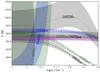 |
Fig. 5 Plasma diagnostics using PyNeb. The dashed or dotted values indicate the density-temperature loci corresponding to the observed reddening-corrected line ratios (also aperture-corrected when combining Spitzer and optical data, as explained in Sect. 4). The coloured bands delineate the one sigma error zones in the corresponding ratios. Diagnostics involving oxygen ions are in green: [O ii]na 3727+/7325+; [O ii]n: 3729/3726; [O iii]na: 5007/4363. Diagnostics involving sulfur ions are in black: [S ii]n: 6716/6731; [S ii]na: 6720+/4072+; [S iii]fn: 18.7 μm/9069; [S iii]na: 9069/6312; the [N ii]na 6584/5755 diagnostic is in blue; the [Ne iii]fn 15.6 μm/3869 diagnostic is in pink; finally the [Fe iii] 5272/4987 diagnostic is in blue. (The characters n, a, f in the denomination of the line ratios stand for “nebular”, “auroral” and “fine-structure”, respectively). |
3.3. Global density structure
The first requirement for a successful photoionization model is to be able to reproduce the observed Hβ surface brightness distribution. We use the Hβ (extinction corrected, continuum subtracted, and flux calibrated) image from Cedrés & Cepa (2002) and assume a uniform electron temperature in order to obtain the surface brightness distribution in two perpendicular directions. The two distributions are quite similar, indicating that the nebula can be assumed to be spherically symmetric. We use this Hβ surface brightness distribution to obtain the density law. We assume spherical symmetry and find that a density law of the type: (1)is convenient to reproduce the observed Hβ surface brightness distribution assuming a constant electron temperature. We find a good fit with A1 = 13 cm-3, A2 = 107 pc, A3 = 1.6, as shown in Fig. 6. Note that in this case we do not consider any filling factor. In the models, the value of A1 is adjusted to reproduce the density and ionization diagnostics, and a filling factor smaller than unity is then needed to reproduce the observed nebular size. In the process of our model fitting, we check that the computed radial temperature variation has not drastically modified the Hβ surface brightness distribution.
4. Photoionization modelling procedure
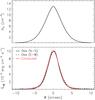 |
Fig. 6 Upper panel: density law needed to fit the Hβ surface brightness distribution assuming a spherical geometry. Lower panel: the observed Hβ surface brightness distribution in two perpendicular directions (black continuous and dotted lines) and the computed one assuming a constant electron temperature. |
The photoionization modeling is performed using the code Cloudy, version c08.01 (Ferland et al. 1998), within the pyCloudy4 environment. With pyCloudy, we can easily obtain the line intensities in specific apertures. The nebula is assumed to be spherically symmetric, with the density distribution described in Sect. 3.3. The stellar ionizing radiation field is obtained as described in Sect. 3.1. The computed line intensities are compared with the observed ones, each in its corresponding aperture. The effects of seeing for the optical data and of minor irregularities in the nebular density distribution are taken into account by convolving with a Gaussian (adopting a width of 1 arcsec for the optical lines and 0.5 arcsec for the infrared lines).
The initial chemical composition of the gas is that derived from collisionally excited lines (and taking t2 = 0) by Bresolin (2007) for O, N, and Ne and by Esteban et al. (2009) for He, S, Cl, Ar, Fe, which were not given by Bresolin. The reason why we use the O, Ne, Ne abundances by Bresolin is due to the potential problem in the [O ii] λ3727 intensity of Esteban et al. (2009) as explained in Sect. 2.2. The carbon abundance is taken equal to the value derived by Bresolin (2007) from the C ii λ4267 recombination line, since there is no other direct information on the carbon abundance.
In the classical logarithmic units taking 12 for hydrogen, the initial composition of the gas is thus: H = 12, He = 10.87, C = 8.66, N = 7.57, O = 8.52, Ne = 7.41, S = 6.91, Cl = 5.50, Ar = 6.35, Fe = 5.74.
Since iron is observed to be strongly depleted in this object, we consider the presence of dust in the model, using the “grains ism” option of Cloudy (but see below for the radial distribution of the grains). In the present object, the effect of grains is essentially to absorb part of the ionizing photons (about 30%) and to heat the gas, especially in the central zone.
A satisfactory model must reproduce the observed Hβ surface brightness distribution law (which in our case it does by construction), the total reddening-corrected Hβ flux and the observed nebular angular size, as well as each of the reddening-corrected observed line ratios in each slit, within the observational uncertainties. We emphasize that it is not sufficient to perform a χ2 fitting of the sum of the deviation of line intensities to the observed value: each line carries its own information, and it is important that all observational constraints be properly accounted for.
Absolute calibration of spectroscopic observations is difficult. We intercalibrate the Spitzer and optical data by forcing the measured value of the H 7–6 / Hβ ratio to the one predicted by our photoionization models in the corresponding slits. The value of f(IR), representing the factor by which the measured IR fluxes have to be multiplied in order for the H 7–6 / Hβ ratio to be in agreement with the model, turns out to be ~1.07. To judge a model, we adopt the same policy as in Morisset & Georgiev (2009) and Stasińska et al. (2010). For each observable O we fix a tolerance τ(O), given by 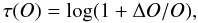 (2)where ΔO/O is the maximum “acceptable” deviation. The values adopted for τ(O) take into account the observational uncertainties and are chosen according to our experience with model fitting. For example, while the observational uncertainty in [O iii] λ5007/[O ii] λ3727 is small, we take a tolerance of 1.15 to reflect the fact that this line ratio is very sensitive to the density distribution and/or the slit position in our object.
Line ratios used to constrain the model and the associated tolerances.
It is convenient to divide the line ratios to be fitted in different categories:
-
ratios of lines measuring the density;
-
ratios of lines measuring the electron temperature;
-
ratios of hydrogen lines or of helium lines, which test the reddening correction, among others;
-
ratios of two different ions of the same element, testing the ionization structure;
-
ratios of lines used to determine the chemical composition, once the ionization structure is correct.
The model is compared to the observations by looking at the values of  (3)which can easily be plotted in the same diagram for all the line ratios. The list of line ratios and associated values of ΔO/O is given in Table 2.
During the fitting procedure, we vary the values of A1, the parameter defining the density (see Sect. 3.3), the filling factor, the total number of ionizing photons (since the proportion of those photons that are absorbed by dust is not known a priori), and the elemental abundances. We also had to modify the spatial distribution of the internal dust. Indeed, when considering a uniform dust-to-gas ratio in the entire nebula, the inner zones became too hot, and the [O iii] λ4363/5007 ratio could not be fitted to gether with the temperature diagnostics of the low excitation zones. We adopted the simplest model for the dust-to-gas ratio, which is a step function. The parameters of the step function were obtained by trial and error to reproduce the observed temperature constraints. Note that such a dust distribution which may seem ad hoc is actually fully justified by the effects of radiation pressure and the possible melting of grains close to the star. That this is precisely what occurs near the Trapezium stars in the Orion nebula was shown already long ago (Baade & Minkowski 1937).
5. Results
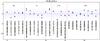 |
Fig. 7 Comparison of model M 1 with the observations. Blue diamonds represent data from Bresolin (2007), green triangles data from Esteban et al. (2009). Red symbols represent ratios involving an infrared line. The dashed and dotted lines represent 1 sigma and 2 sigmas deviations, respectively. |
5.1. The simplest model
In order to constrain the model-fitting we took the observations by Bresolin (2007), using the data of Esteban et al. (2009) as a complement. The most satisfactory model we produced, within the explained procedure, is one having A1 = 200 cm-3, a filling factor of 0.005, and a total number of ionizing photons Q(H) = 5.9 × 1051 s-1.
A graphical representation of how the line-ratio constraints match the data is shown in Fig. 7: the values of κ(O) are plotted for all the constraints O. Diamonds correspond to intensities from the Bresolin (2007) spectrum, triangles to intensities from the Esteban et al. (2009) optical spectrum, each one within its extraction aperture. It can be seen that each of the values of κ(O) is found to lie between −2 and + 2 (except for the [S iv] λ10.5 μm/[S iii] λ18.7 μm ratio, and the [O iii] λ5007/Hβ ratio from Bresolin 2007). A more conventional comparison of our best model, M1, with the observed line ratios is shown in Table 3. It can be seen that the κ(O) values for Bresolin (2007) and Esteban et al. (2009) are slightly different, which means that either the density distribution in the model is too simplistic (i.e. that some slight density inhomogeneities are present) or that the observational error bars are slightly underestimated. Probably both reasons are relevant, but in any case the differences are small (except for the case of the [O ii] λ3727 line mentioned above).
The elemental abundances in this model are: H = 12, He = 10.97, C = 8.66, N = 7.79, O = 8.42, Ne = 7.80, S = 6.98, Cl = 5.18, Ar = 6.20, Fe = 5.77. They differ from the initial ones, mainly due to the fact that the classical ionization correction factors used to derive abundances by Bresolin (2007) or Esteban et al. (2009) are not in agreement with our photoionization model. Such an explanation, obviously, does not hold for oxygen, because both O+ and O++ lines are measured. Yet, there is a 0.1 dex difference between the model value and the value derived by Bresolin (2007). The reason is that this model is not perfect, because it cannot reproduce at the same time all the line ratios involving [O iii] λ5007.
In Fig. 9 we show the radial distribution of the electron temperature, the dust-to-gas ratio, the hydrogen density, and the relative abundances of O+ and O++ in model M1 (red curves). We see that the radial gradient of the electron temperature is mild, with a temperature of ≃ 7200 K in the central zone and ≃ 7700 K in the outer zone. This is what we would have expected for an H ii region of roughly solar metallicity. The important point is that this temperature distribution is fully compatible with the line intensities observed both in the optical and in the infrared. The small increase of the electron temperature at 2 × 1020 cm is due to photoelectric heating of the gas by dust grains. We have checked that the amount of dust present in the model is compatible with the extinction C(Hβ) ≃ 0.3 estimated for this object from the Balmer lines.
We note that the intensity of the [O i] λ6300 line is smaller by a factor ~10 compared to the observations. This does not represent a real worry, since [O i] is essentially produced in the ionization front (i.e. not in the ionized regions as all the remaining lines), and we did not attempt to model this zone in detail.
The discussion of the recombination lines is postponed to Sect. 5.3.
5.2. A composite model
One problem that still needs examination is the density structure. Our best model, M1, requires a volume filling factor of 0.005. This is not uncommon for giant H ii regions (e.g. Luridiana et al. 1999; Stasińska & Schaerer 1999). Of course, using a filling factor is an approximation. There has to be some diffuse gas between the filaments. We have to check whether such gas affects the intensities of the observed emission lines. We have thus computed additional low-density models with the same abundances at the “high” density, main model. The computations are performed until the outer radius of the nebula is reached (so, for low densities, these additional models are density bounded). A composite model is then obtained by adding the fluxes of the main, “high” density model, with one of those additional models. This is, of course, a simplification of a more realistic model where the density distribution would be filamentary (as in the model of Jamet et al. 2006), but it is sufficient for our purposes. The results of our “best fit” composite model, M2, are shown in Fig. 8 and Table 3. The high- and low-density components have A1 = 235 and A1 = 5 cm-3, and filling factors of 0.003 and 0.5, respectively.
Characteristics of the corresponding low-density model are plotted in Fig. 9, with blue curves. From Fig. 8 we see that our best composite model fits the data even better than model M1. In particular, the [S iv]10.5/[S iii]18.7 and the [O iii] λ5007/Hβ ratio from Bresolin (2007) are now well fitted. This is not too surprising, since we have allowed more parameters to vary and the resulting model should be closer to reality. Since, for the composite model, we have adopted the same dust-to-gas ratio distribution as for model M1, the jump in electron temperature at the place where grains appear is much higher than in model M1, because, as a consequence of the higher local ionization parameter due to the lower gas density, the effect of heating by grains is enhanced (Stasińska & Szczerba 2001). Note that, in the central zone, devoid of grains, the temperature of the low-density model is lower than in the case of model M1. This is because oxygen is entirely in the form of O++, the most efficient coolant. In spite of the significant differences in temperatures with model M1, the overall “temperature fluctuation” t2 (as defined by Peimbert 1967, and computed by us integrating the temperature weighted by the product nenH over the emitting volume) is very small in this composite medel (less than 0.001). We have to note that, although other composite models can probably be found to fit all the observations equally well, they will not differ significantly from M2 because of the very strong constraints imposed on each zone of the nebula by the observations.
The chemical composition of the composite model is: H = 12, He = 11.0, C = 8.66, N = 7.74, O = 8.57, Ne = 7.84, S = 6.87, Cl = 5.27, Ar = 6.23, Fe = 5.87.
We do not attempt here to assign error bars to the abundances derived from the model, as this would require to perfectly fit the models to various combinations of the extreme values of intensities allowed by the observations. This represents a very time consuming task, because line intensities are not directly proportional to abundances. Fortunately, we do not need to go through such a lengthy procedure. What we wanted is to see whether we can obtain at least one photoionization model including all the classical ingredients which would fit all the observations, including the new infrared data, which put strong constraints on the temperature. The fact that we succeeded argues against the presence of important temperature inhomogeneities in this object.
5.3. Recombination lines and temperature fluctuation issues
Let us now look at the recombination lines of C and O as predicted by our models. The C ii] λ 4267 line is well reproduced by our models, which indicates that the ionization correction factors used by both Bresolin (2007) and Esteban et al. (2009) to derive the carbon abundance are in agreement with our model predictions. This, however, does not mean that the carbon abundance is correct, since one might expect a similar problem with the carbon recombination line as with the oxygen ones. Indeed, the sum of the intensities of multiplet 1 of O ii (labelled O ii] λ 4651 in Table 3) is about 4 times smaller than the observed value (if we use Eq. (11) from Peimbert et al. 2005; to convert the intensity of O ii λ 4649 observed by Esteban et al. 2009 into the sum of the multiplet). This is because the oxygen abundance in the models is fixed by fitting the observed intensities of the forbidden lines. Thus, the oxygen abundance discrepancy between the recombination lines and collisionally excited lines appears to be of a factor of 0.6 dex5. That the models underpredict the value for O ii λ 4651 is not surprising, since they are chemically homogeneous and do not experience sufficient temperature variations to explain the observed O++/H+ abundance discrepancy.
Observed line ratios in H 1013 compared to the results of models M1 and M2.
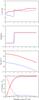 |
Fig. 9 Radial distribution of the electron temperature, the dust-to-gas ratio, the hydrogen density, and the relative abundances of O+ (dashed curve) and O++ (continuous curve). The thick red curves correspond to Model M1 (or the high-density component of model M2) while the thin blue curves correspond to the low density component of model 2. |
We have made some experiments by enhancing the oxygen abundance so as to reproduce O ii λ 4651. Oxygen cooling is then so important that it lowers the gas temperature to such a point where the [O iii] λ5007 line becomes severely underestimated. In addition, if the oxygen abundance is enhanced by a factor of 3 of 4 with respect to the solar value, from what is known of stellar nucleosynthesis and galactic chemical evolution, this should also be the case of other α-elements, such as neon, sulfur and argon. In this case, the intensitiy of the [S iii] λ18.7 μm line becomes largely overestimated.
Our models also do not explain the Balmer jump temperature of 5000 ± 800 K obtained by Bresolin (2007), which led to his t2 = 0.06. However, it must be noted that the spectral resolution of Bresolin’s observations was not sufficient to reach an accurate value of the level of the continuum close to the Balmer discontinuity as well as of the intensity of the high-order Balmer lines, so that the Balmer jump with respect to adjacent hydrogen lines could be easily overestimated by 20%, leading in that case to a Balmer jump temperature close to 7000 K. The spectrum of Esteban et al. (2009) is an echelle spectrum with much higher spectral resolution but poor signal-to-noise ratio in the continuum, so unfortunately the Balmer jump could not be measured there.
6. Conclusion
In order to get more insight into the “temperature fluctuation” and the “abundance discrepancy” problems we have performed a detailed study of the giant H ii region H 1013, for which excellent spectroscopic data exist, and which has been previously diagnosed for the presence of temperature fluctuations. We have first completed the observational data base with our own mid-infrared measurements using the Spitzer Space Telescope, which give us important additional constraints, especially on the temperature structure.
We then made a first estimate of the physical parameters (electron density and temperature) from different line ratios including the ones involving the infrared data using the PyNeb software (Luridiana et al. 2012). This indicated that temperature fluctuations, even if present, would be much smaller than t2 = 0.06 invoked by Bresolin (2007) from the Balmer jump temperature or t2 = 0.04 from the O++ abundance discrepancy obtained by comparison of the recombination and collisionally excited lines from the high resolution spectrum of Esteban et al. (2009).
For a deeper insight, one needs to carry out a detailed photoionization analysis in which all the processes that affect the line intensities as well as the observing apertures are taken into account. We performed such a study, using Starburst99 and the pyCloudy package, trying to find a photoionization model of H 1013 that is able to reproduce all the observational data (surface brightness distribution, line ratios and stellar features).
We were able to produce an almost satisfactory model, assuming a volume filling factor of 0.005. Since the use of a filling factor is just a zero-order approach, we checked the effect of adding a low-density medium to the modelled clumps or filaments. This resulted in an even better fit to the observations. Of course, as in any study which requires the inclusion of a volume filling factor or – more realistically – with a large volume of diffuse gas bathing the filaments, we are left with the question of what continuously generates those filaments, since their lifetime must be short, as they are not in pressure equilibrium with the surrounding diffuse matter.
The fact that we are able to produce photoionization models that perfectly fit most observational constraints – which are strong and numerous – argues against the presence of significant temperature fluctuations in H 1013, contrary to what has been advocated previously for this object. The oxygen abundance of our best model is 12 + log O/H = 8.57, as opposed to the values of 8.73 and 8.93 advocated by Esteban et al. (2009) and Bresolin (2007), respectively.
However, our model is not able to reproduce the intensities of the oxygen recombination lines, which is one of the big things that remain to be explained. Our model also does not reproduce the very low Balmer jump temperature inferred by Bresolin (2007) from his data, but we have argued that his value might be in error, possibly due to insufficient spectral resolution of the observations for such a purpose. A new observational study, focussing on the Balmer jump temperature in this nebula, would obviously be very important for our case.
This paper can by no means be considered a solution to the nagging “temperature fluctuation” and “abundance discrepancy” problems, since it studies just one object and does not even provide a complete understanding of the observational data. But it serves as a warning against too general statements about the physical conditions in H ii regions and too hasty conclusions drawn from their spectra. A promising solution is of course the deviation from a Maxwellian distribution of electron energies, proposed by Nicholls et al. (2012). Work in this direction is needed to show quantitatively that such circumstances i) can occur in H ii regions; and ii) are able to produce photoionization models that reproduce a wide range of observational constraints, as we have attempted.
Here, and in the remainder of the text, 3727+ stands for 3726 + 3729.
IRAF is distributed by the National Optical Astronomy Observatories, which are operated by the Association of Universities for Research in Astronomy, Inc., under cooperative agreement with the National Science Foundation.
This combination of ages does not have to correspond to reality since, as explained above, we are in the regime where statistical fluctuations matter. The important thing is that the spectral energy distribution of the ionizing radiation field is correct.
pyCloudy is the python version of Cloudy_3D (Morisset 2006) available at https://sites.google.com/site/pycloudy/
This is larger than the value of 0.36 dex derived by Esteban et al. (2009) from their observations due to the conjunction of several causes such as the fact that our model attempts to fit the observation of Bresolin (2007) rather than those of Esteban et al. (2009), and that Esteban (priv. comm.) did not employ the same procedure to estimate the sum of the multiplet.
Acknowledgments
We wish to thank B. Cedrés and J. Cepa for sharing with us the ALFOSC images of M101 and Ryszard Szczerba for helping with the Spitzer spectrum. S.S.-D. acknowledges financial support by the Spanish Ministerio de Ciencia e Innovación under the project AYA2008-06166-C03-01 and the Spanish MICINN under the Consolider-Ingenio 2010 Program grant CSD2006-00070: First Science with the GTC (http://www.iac.es/consolider-ingenio-gtc). G.S. and C.M. acknowledge support from the following Mexican projects: CB2010:153985, PAPIIT-IN105511 and PAPIIT-IN112911. This work is based in part on observations made with the Spitzer Space Telescope, which is operated by the Jet Propulsion Laboratory, California Institute of Technology, under a contract with NASA. Support for this work was provided by NASA through an award issued by JPL/Caltech.
References
- Aller, L. H., & Menzel, D. H. 1945, ApJ, 102, 239 [NASA ADS] [CrossRef] [Google Scholar]
- Baade, W., & Minkowski, R. 1937, ApJ, 86, 119 [NASA ADS] [CrossRef] [Google Scholar]
- Bresolin, F. 2007, ApJ, 656, 186 [NASA ADS] [CrossRef] [Google Scholar]
- Cedrés, B., & Cepa, J. 2002, A&A, 391, 809 [NASA ADS] [CrossRef] [EDP Sciences] [Google Scholar]
- Cerviño, M., Luridiana, V., Pérez, E., Vílchez, J. M., & Valls-Gabaud, D. 2003, A&A, 407, 177 [NASA ADS] [CrossRef] [EDP Sciences] [Google Scholar]
- Esteban, C., Bresolin, F., Peimbert, M., et al. 2009, ApJ, 700, 654 [NASA ADS] [CrossRef] [Google Scholar]
- Ferland, G. J., Korista, K. T., Verner, D. A., et al. 1998, PASP, 110, 761 [Google Scholar]
- García-Rojas, J., & Esteban, C. 2007, ApJ, 670, 457 [NASA ADS] [CrossRef] [Google Scholar]
- Jamet, L., Pérez, E., Cerviño, M., et al. 2004, A&A, 426, 399 [NASA ADS] [CrossRef] [EDP Sciences] [Google Scholar]
- Jamet, L., Stasińska, G., Pérez, E., González Delgado, R. M., & Vílchez, J. M. 2005, A&A, 444, 723 [NASA ADS] [CrossRef] [EDP Sciences] [Google Scholar]
- Kroupa, P. 2001, MNRAS, 322, 231 [NASA ADS] [CrossRef] [Google Scholar]
- Luridiana, V., Peimbert, M., & Leitherer, C. 1999, ApJ, 527, 110 [NASA ADS] [CrossRef] [Google Scholar]
- Luridiana, V., Morisset, C., & Shaw, R. A. 2012, in Planetary Nebulae: an Eye to the Future (Cambridge University Press), IAU Symp., 283 [Google Scholar]
- Mesa-Delgado, A., Núñez-Díaz, M., Esteban, C., et al. 2012, MNRAS, 426, 614 [NASA ADS] [CrossRef] [Google Scholar]
- Morisset, C. 2006, IAUS, 234, 467 [Google Scholar]
- Morisset, C., & Georgiev, L. 2009, A&A, 507, 1517 [NASA ADS] [CrossRef] [EDP Sciences] [Google Scholar]
- Nicholls, D. C., Dopita, M. A., & Sutherland, R. S. 2012, ApJ, 752, 148 [NASA ADS] [CrossRef] [Google Scholar]
- Osterbrock, D. E. 1989, Astrophysics of gaseous nebulae and active galactic nuclei (Mill Valey, CA: University Science Books) [Google Scholar]
- Peimbert, M. 1967, ApJ, 150, 825 [NASA ADS] [CrossRef] [Google Scholar]
- Peimbert, M., & Costero, R. 1969, BOTT, 5, 3 [Google Scholar]
- Peimbert, M., & Peimbert, A. 2011, RMxAC, 39, 1 [NASA ADS] [Google Scholar]
- Stasińska, G. 2005, A&A, 434, 507 [NASA ADS] [CrossRef] [EDP Sciences] [Google Scholar]
- Stasińska, G. 2004, in Cosmochemistry: The Melting Pot of the Elements, eds. C. Esteban, R. J. García López, A. Herrero, & F. Sánchez (Cambridge: Cambridge Univ. Press), 115 [Google Scholar]
- Stasińska, G. 2009, in The Emission-Line Universe: XVIII Canary Islands Winter School of Astrophysics, ed. J. Cepa (Cambridge University Press), 1 [Google Scholar]
- Stasińska, G., & Schaerer, D. 1999, A&A, 351, 72 [NASA ADS] [Google Scholar]
- Stasińska, G., & Szczerba, R. 2001, A&A, 379, 1024 [NASA ADS] [CrossRef] [EDP Sciences] [Google Scholar]
- Stasińska, G., Tenorio-Tagle, G., Rodríguez, M., & Henney, W. J. 2007, A&A, 471, 193 [NASA ADS] [CrossRef] [EDP Sciences] [Google Scholar]
- Stasińska, G., Morisset, C., Tovmassian, G., et al. 2010, A&A, 511, A44 [NASA ADS] [CrossRef] [EDP Sciences] [Google Scholar]
- Storey, P. J., & Hummer, D. G., 1995, MNRAS, 272, 41 [NASA ADS] [CrossRef] [Google Scholar]
- Torres-Peimbert, S., & Peimbert, M. 2003, IAUS, 209, 363 [NASA ADS] [Google Scholar]
- Tsamis, Y. G., & Péquignot, D. 2005, MNRAS, 364, 687 [NASA ADS] [CrossRef] [Google Scholar]
All Tables
All Figures
|
Fig. 1 Portion of the Hα continuum-subtracted image of M 101 presented by Cedrés & Cepa (2002) showing the H ii region H 1013. The apertures corresponding to the optical and infrared spectra used in this study are also indicated for reference: the long narrow one corresponds to the LRIS data, the short narrow one to the HIRES data, and the wide one to the mid-infrared observations (note that the slit orientation is arbitrary). |
| In the text | |
|
Fig. 2 The WR features in the optical spectrum of Bresolin (2007). |
| In the text | |
|
Fig. 3 Spitzer Space Telescope spectrum of H 1013. |
| In the text | |
|
Fig. 4 Time dependence of several characteristics of an instantaneous starburst of solar metallicity obtained with Starburst99 (see text for details). The observed values or their upper limits in H 1013 are shown respectively by green and magenta horizontal lines. |
| In the text | |
|
Fig. 5 Plasma diagnostics using PyNeb. The dashed or dotted values indicate the density-temperature loci corresponding to the observed reddening-corrected line ratios (also aperture-corrected when combining Spitzer and optical data, as explained in Sect. 4). The coloured bands delineate the one sigma error zones in the corresponding ratios. Diagnostics involving oxygen ions are in green: [O ii]na 3727+/7325+; [O ii]n: 3729/3726; [O iii]na: 5007/4363. Diagnostics involving sulfur ions are in black: [S ii]n: 6716/6731; [S ii]na: 6720+/4072+; [S iii]fn: 18.7 μm/9069; [S iii]na: 9069/6312; the [N ii]na 6584/5755 diagnostic is in blue; the [Ne iii]fn 15.6 μm/3869 diagnostic is in pink; finally the [Fe iii] 5272/4987 diagnostic is in blue. (The characters n, a, f in the denomination of the line ratios stand for “nebular”, “auroral” and “fine-structure”, respectively). |
| In the text | |
|
Fig. 6 Upper panel: density law needed to fit the Hβ surface brightness distribution assuming a spherical geometry. Lower panel: the observed Hβ surface brightness distribution in two perpendicular directions (black continuous and dotted lines) and the computed one assuming a constant electron temperature. |
| In the text | |
|
Fig. 7 Comparison of model M 1 with the observations. Blue diamonds represent data from Bresolin (2007), green triangles data from Esteban et al. (2009). Red symbols represent ratios involving an infrared line. The dashed and dotted lines represent 1 sigma and 2 sigmas deviations, respectively. |
| In the text | |
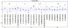 |
Fig. 8 Comparison of the composite model, M 2, with the observations. Same layout as in Fig. 7. |
| In the text | |
|
Fig. 9 Radial distribution of the electron temperature, the dust-to-gas ratio, the hydrogen density, and the relative abundances of O+ (dashed curve) and O++ (continuous curve). The thick red curves correspond to Model M1 (or the high-density component of model M2) while the thin blue curves correspond to the low density component of model 2. |
| In the text | |
Current usage metrics show cumulative count of Article Views (full-text article views including HTML views, PDF and ePub downloads, according to the available data) and Abstracts Views on Vision4Press platform.
Data correspond to usage on the plateform after 2015. The current usage metrics is available 48-96 hours after online publication and is updated daily on week days.
Initial download of the metrics may take a while.