| Issue |
A&A
Volume 551, March 2013
|
|
|---|---|---|
| Article Number | A6 | |
| Number of page(s) | 10 | |
| Section | Astrophysical processes | |
| DOI | https://doi.org/10.1051/0004-6361/201220359 | |
| Published online | 08 February 2013 | |
No anticorrelation between cyclotron line energy and X-ray flux in 4U 0115+634
1 Dr. Karl Remeis-Observatory & ECAP, Universität Erlangen-Nürnberg, Sternwartstr. 7, 96049 Bamberg, Germany
e-mail: This email address is being protected from spambots. You need JavaScript enabled to view it.
2 ISDC Data Center for Astrophysics, University of Geneva, 16 chemin d’Écogia, 1290 Versoix, Switzerland
3 Leibniz-Institut für Astrophysik Potsdam, An der Sternwarte 16, 14482 Potsdam, Germany
4 School of Physics, Astronomy, and Computational Sciences, MS 5C3, George Mason University, 4400 University Drive, Fairfax, VA 22030, USA
5 Space Science Division, Naval Research Laboratory, Code 7655, 4555 Overlook Ave., S.W., Washington, DC 20375, USA
6 CEA Saclay, DSM/IRFU/SAp-UMR AIM (7158) CNRS/CEA/Université Paris 7, Diderot, 91191 Gif-sur-Yvette, France
7 CRESST and NASA Goddard Space Flight Center, Greenbelt, MD 20771, USA, and Center for Space Science and Technology, UMBC, Baltimore, MD 21250, USA
8 Space Radiation Laboratory, 290-17 Cahill, Caltech, 1200 East California Blvd., Pasadena, CA 91125, USA
9 Center for Astrophysics and Space Sciences, University of California, San Diego, La Jolla, CA 92093, USA
10 Instituto Universitario de Física Aplicada a las Ciencias y las Tecnologías, University of Alicante, PO Box 99, 03080 Alicante, Spain
11 Institut für Astronomie und Astrophysik, Universität Tübingen, Sand 1, 72076 Tübingen, Germany
Received: 10 September 2012
Accepted: 23 November 2012
Abstract
We report on an outburst of the high mass X-ray binary 4U 0115+634 with a pulse period of 3.6 s in 2008 March/April as observed with RXTE and INTEGRAL. During the outburst the neutron star’s luminosity varied by a factor of 10 in the 3–50 keV band. In agreement with earlier work we find evidence of five cyclotron resonance scattering features at ~10.7, 21.8, 35.5, 46.7, and 59.7 keV. Previous work had found an anticorrelation between the fundamental cyclotron line energy and the X-ray flux. We show that this apparent anticorrelation is probably due to the unphysical interplay of parameters of the cyclotron line with the continuum models used previously, e.g., the negative and positive exponent power law (NPEX). For this model, we show that cyclotron line modeling erroneously leads to describing part of the exponential cutoff and the continuum variability, and not the cyclotron lines. When the X-ray continuum is modeled with a simple exponentially cutoff power law modified by a Gaussian emission feature around 10 keV, the correlation between the line energy and the flux vanishes, and the line parameters remain virtually constant over the outburst. We therefore conclude that the previously reported anticorrelation is an artifact of the assumptions adopted in the modeling of the continuum.
Key words: X-rays: binaries / pulsars: individual 4U 0115+634 / magnetic fields
© ESO, 2013
1. Introduction
In all accreting X-ray pulsars the accretion geometry is strongly affected by the magnetic field of the neutron star, which has values of a few 1012 G at the magnetic poles. The accreted matter is forced to follow the magnetic field lines from the Alfvén radius inward to the accretion columns located at the magnetic poles of the neutron star. The shape of these columns remains an open question. The simplest models assume cylinder or slab-like geometries, although more complicated shapes have been discussed (Mészáros 1984; Becker et al. 2012). On each magnetic pole of the neutron star, a hot spot is created, emitting thermal photons into the accretion column (Davidson 1973). These photons are upscattered in energy by inverse Compton scattering within the accretion column, forming the hard X-ray spectrum (Becker & Wolff 2007; Ferrigno et al. 2009). Depending on the source luminosity, and thus mass accretion rate, Ṁ, and deceleration mechanism, a radiation-dominated shock can form above the surface of the neutron star. See Becker et al. (2012) for a discussion of the different modes of accretion in the accretion column.
Owing to the strong magnetic field of accreting X-ray pulsars, cyclotron resonance scattering features (cyclotron lines; CRSFs) are observable in many X-ray pulsars. These features have been reported for about 20 X-ray pulsars (Caballero & Wilms 2011). CRSFs are produced by photons generated in the accretion column of the neutron star interacting with electrons (Schönherr et al. 2007; Mészáros 1992, and references therein). The motion of these electrons perpendicular to the B-field is quantized into Landau levels with energy differences of about  (1)Photons inelastically scattering off these electrons will imprint absorption-line like features onto the spectral continuum.
Measuring the energy of the CRSF yields information about the B-field strength in the line forming region. Since the B-field of a neutron star can be assumed to be dipole-like to first order, in many models the centroid energy of CRSFs depends on the characteristic emission height, i.e., the altitude of the line forming region (Basko & Sunyaev 1976; Burnard et al. 1991; Mihara et al. 2004). Since this altitude depends on the complex relation between the deceleration of the accreted material and the mass accretion rate, it is expected to depend on the source luminosity. Such a dependence has indeed been observed. Three types of behavior have been observed. One type shows a positive correlation between the X-ray luminosity LX and the cyclotron line energy Ecyc (e.g., Her X-1, Staubert et al. 2007). The other type shows a negative correlation between LX and Ecyc (e.g., V0332+53, Nakajima et al. 2010, and references therein). Finally, there are also cyclotron sources known with a constant cyclotron line energy (e.g., A0535+26, Caballero et al. 2007).
As suggested by Staubert et al. (2007) and Klochkov et al. (2011) and then quantified by Becker et al. (2012), these different relations between LX and Ecyc could be due to the different deceleration mechanisms for the accreted material. Above a certain critical luminosity, Lcrit, the accreted material is decelerated mainly by the radiation pressure. In this situation, an increase in luminosity stops the material earlier, leading to the line forming region being in a region of lower B-field strength and yielding a negative correlation between Ecyc and LX. For very low luminosities, the deceleration is dominated by the gas pressure. In this regime higher mass accretion rates will compress the accretion mound and thus lead to a positive correlation between the luminosity and the cyclotron line energy. Finally, at intermediate luminosities one expects a regime where the accretion column is fairly stable and the deceleration is dominated by Coulomb interactions.
4U 0115+634 (Giacconi et al. 1972) is one of the X-ray pulsars for which CRSFs have been studied in great detail (see, e.g., Wheaton et al. 1979; White et al. 1983; Nagase et al. 1991; Heindl et al. 1999; Santangelo et al. 1999; Mihara et al. 2004; Nakajima et al. 2006; Tsygankov et al. 2007; Ferrigno et al. 2009, 2011). The source shows 3.61 s pulsation and has an orbital period of ~24.3 d (Cominsky et al. 1978; Rappaport et al. 1978). The optical counterpart is the O9e star V635 Cas (Johns et al. 1978; Unger et al. 1998).
In previous outbursts, CRSFs have been detected up to the fifth harmonic (Heindl et al. 2000). This is the largest number of detected CRSFs in an accreting X-ray pulsar. In later work, a negative correlation between LX and Ecyc was found (e.g., Nakajima et al. 2006; Tsygankov et al. 2007; Müller et al. 2010), meaning that the source should be located in the supercritical luminosity regime. Other authors even found a discontinuous behavior of the fundamental line energy and explained this by a sudden change of the accretion conditions (Li et al. 2012).
In this work we revisit the behavior of the CRSFs in 4U 0115+634. Focusing on data taken during a giant outburst in 2008 March/April (Fig. 1). We show that the previously claimed relation between the source flux FX and Ecyc strongly depends on the choice of the underlying continuum model. In Sect. 2 we summarize the observations. In Sect. 3 we describe the different continuum models and the flux and time dependence of the continuum and cyclotron line parameters. We argue that the cyclotron line is only modeled correctly when using an exponentially cutoff power law continuum with a strong emission feature around 10 keV. Furthermore, alternative continua models, which have been used in some earlier investigations, result in incorrect cyclotron line parameters which can cause the apparent relation between source flux FX and fundamental cyclotron line energy E0. We summarize this paper in Sect. 5.
2. Observations and data reduction
The outburst of 4U 0115+634 started 2008 March 12, after a phase of almost four years of quiescence, when Swift/BAT detected a significant increase of the X-ray flux (Krimm et al. 2008). The outburst lasted about 40 days and exceeded a flux of ~200 mCrab in the 2–12 keV RXTE/ASM band (Fig. 1). The whole outburst was monitored with pointed observations by the Rossi X-ray Timing Explorer (RXTE, Bradt et al. 1993) and several pointed observations by the INTErnational Gamma-Ray Astrophysics Laboratory (INTEGRAL, Winkler et al. 2003). Here, we use data from RXTE’s Proportional Counter Array (PCA, Jahoda et al. 2006) and the High Energy X-Ray Timing Experiment (HEXTE, Rothschild et al. 1998), as well as the INTEGRAL Soft Gamma-Ray Imager (ISGRI, Lebrun et al. 2003). Data were reduced with our standard analysis pipelines, based on HEASOFT (v. 6.11) and INTEGRAL OSA v. 9.0. Data modeling was performed with the newest version of the Interactive Spectral Interpretation System (ISIS, Houck & Denicola 2000).
The PCA consisted of five proportional counter units (PCUs), which were sensitive between 2 and 60 keV. Since PCU 2 is known to have been the best calibrated one (Jahoda et al. 2006), we only extracted spectra from the top layer of this PCU in the standard2f mode. The hard X-ray spectrum from 15–250 keV was monitored with HEXTE. HEXTE consisted of two independent clusters, A and B, both arrays of four phoswich scintillation detectors. The “rocking mechanism” of these clusters allowed a near realtime measurement of the background. Since this mechanism failed for cluster A before our observations, we only used data from cluster B. The other instrument for the hard X-rays was the pixelized CdTe detector ISGRI behind a Coded Mask on board the INTEGRAL satellite. It covers the energy range between ~18 keV and 1 MeV. We extracted all available ISGRI spectra, for which 4U 0115+634 was less than 10° off-axis. Table 1 contains an observation log (see also Fig. 1).
Log of observations for the 2008 outburst of 4U 0115+634.
 |
Fig. 1 RXTE/ASM lightcurve of 4U 0115+634 (2–12 keV). The inset shows a close-up view of this lightcurve, showing the 2008 outburst in detail. Arrows indicate the times of pointed RXTE and INTEGRAL observations. Numbers indicate the observation epochs used in the data analysis (see also Table 1). |
For the spectral analysis we used data between 3 and 50 keV for PCA, and between 20 and 100 keV for HEXTE and for ISGRI. A systematic error has been added in quadrature to the PCA and ISGRI data, using the canonical values of 0.5% and 2.0% (Jahoda et al. 2006, and IBIS Analysis User Manual1), respectively. To improve the signal to noise ratio of the spectra, we averaged the data over 14 data blocks in time. These data blocks are defined in the fifth column of Table 1 and shown in Fig. 1. We omitted one ISGRI dataset from our analysis (revolution number 677), because no simultaneous RXTE data are available at that time and the source was almost in the off state during that observation.
3. Spectral analysis
3.1. Pulsar continuum models
A large problem when analyzing X-ray spectra from X-ray binary pulsars is to find a good description of the broadband continuum. In most cases, semi-physical models, which are some variant of a power law with a high energy exponential cutoff (Kreykenbohm et al. 2002, and references therein), are used to describe the spectra. These models can be justified by considering the Comptonization of soft photons in an accretion column (Becker & Wolff 2007, and references therein). The most basic exponentially cutoff power law model, called CutoffPL in ISIS and XSPEC (Arnaud 1996), has the form  (2)with the photon index, Γ, and the folding energy, Efold (see, e.g., Schönherr et al. 2007). However, this simple model is often, but not always, insufficient to describe the continua of observed X-ray pulsars, as the curvature in the continuum is often seen to start at different energies. To obtain a good spectral fit, therefore, models with more free fit parameters and more complex shapes are sometimes required. The most simple of these models is the power law with high energy cutoff
 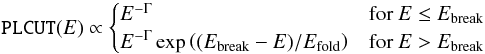 (3)where for typical X-ray pulsars Ebreak ~ 10 keV and which has an unphysical “kink” at Ebreak, which can result in line-like residuals around this energy (Kretschmar et al. 1997; Kreykenbohm et al. 1999). For this reason Klochkov et al. (2008) and Ferrigno et al. (2009) smooth the continuum around this break, using a model of the form
 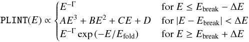 (4)where the coefficients A, B, C, and D are chosen such that the continuum and its first derivative are continuous at E = Ebreak ± ΔE and where ΔE ≠ 0 but sufficiently small.
Other common choices to avoid the break are the so called negative and positive power-law exponential (NPEX, see, e.g., Makishima et al. 1999, and references therein), a continuum model with five free parameters of the form  (5)with photon indices Γ1,2 ≥ 02, and the “Fermi Dirac cutoff” (FDCUT, see Tanaka 1986)
  (6)Common to all of these empirical continua is that despite the smoother transition around Ebreak they often need to be modified further by a broad excess or depression around 10 keV. This so-called “10 keV feature” has been observed in many X-ray pulsar spectra, either in absorption or in emission, although its origin is still not clear (Coburn 2001). This feature is usually modeled as an additive Gaussian line, with the centroid energy EG, the width σG, and the flux AG.
In addition to those empirical models, based on the theoretical description of bulk and thermal Comptonization in magnetized accretion columns of Becker & Wolff (2007, and references therein), Ferrigno et al. (2009) have developed a continuum model depending on physical parameters like the column radius, the accretion rate, the electron temperature, the B-field strength. A hybrid model which combines the broadband continuum with CRSFs is currently in preparation (Schwarm et al., in prep.). These physics-based continuum models are still in active development and, because of the large number of free parameters, only suited for very high signal to noise data. For this reason most observational work uses one of the continua described by Eqs. (2)–(6).
For sources with cyclotron lines, the continuum model is modified with a description of the cyclotron line. Since physically self consistent line models such as those described by Schönherr et al. (2007) are still not available for all sources, empirical line models are generally used. The two most common CRSF models are those using a Gaussian or a pseudo-Lorentzian profile (see discussion by Nakajima et al. 2010). Here, we model the CRSFs with a pseudo-Lorentzian optical depth profile (Mihara et al. 1990), i.e., we multiply the continuum model with  (7)with the centroid energy, Ecyc, the width of the feature, W, and the optical depth of the line, τ. This approach allows the comparison of the line parameters with results from previous papers, in which also the CYCLABS model has been used (e.g., Nakajima et al. 2006; Tsygankov et al. 2007; Li et al. 2012). In the remainder of the paper, we label the cyclotron line parameters with the number of respective harmonic, where 0 corresponds to the fundamental line. As common for CRSFs, W and τ are strongly correlated (Coburn 2001). We therefore set a lower limit of 0.5 keV for the width, which is comparable to the typical PCA resolution.
In order to describe the data of 4U 0115+634, in addition to several of the continuum models discussed above, we take interstellar absorption into account, modeling it with an updated version of TBabs3, using abundances by Wilms et al. (2000) and cross sections by Verner & Yakovlev (1995). We furthermore account for an intrinsic Fe Kα fluorescence line, which we describe with an additive narrow Gaussian emission line with frozen centroid energy at 6.4 keV, a width of 10-4 keV, and a flux AFe and equivalent width WFe. Assuming a narrow line is justified because in systems like 4U 0115+63 Fe Kα is expected to have a width on the order of ≲ 0.5 keV (see, e.g., Torrejón et al. 2010), which cannot be resolved by PCA.
In order to take into account that the flux normalization of the different instruments used is not perfectly known we introduce cross calibration constants cHEXTE and cISGRI as free fit parameters. These constants also account for flux differences of the source between the observations which were not fully simultaneous. The PCA background was estimated using the standard models provided by GSFC. These estimates often show a flux deviation from the proper background by a few percent. This deviation was accounted for by multiplying the background flux with another fit parameter, cb (see also Rothschild et al. 2011).
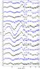 |
Fig. 2 Deviations between the data and the best fit with CutoffPL and 10 keV feature for the PCA (circles), HEXTE (crosses), and ISGRI (filled diamonds) in units of standard deviations σ. For these fits, no cyclotron lines have been taken into account. The numbers on the right side indicate the respective epoch. |
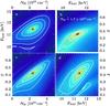 |
Fig. 3 a) c) and d) Confidence contours for the folding energy, the photon index and the hydrogen column density for epoch 6. b) Confidence contours between the Efold and Γ with NH frozen to 1.7 × 1022 cm-2. Contour lines correspond to the 68.3%, 90%, and 99% level. Color indicates Δχ2 with respect to the best fit value, with the color scale running from orange (low Δχ2) to dark blue (large Δχ2). |
3.2. Fitting strategy
Since the CutoffPL is the easiest continuum model for X-ray pulsars, we used this model for our fits. Furthermore, the 10 keV feature in emission is required to get a good description of the data. For each epoch, the fits have been simultaneously performed for all available instruments. Figure 2 shows the residuals of the best fit using this continuum without taking any CRSFs into account. These residuals clearly indicate the need of the cyclotron lines in this model at ~11, 22, and sometimes above 30 keV. As the quality of individual data sets is strongly variable over the outburst, in an initial fit run a variable number of CRSFs were added to individual fits until the reduced χ2,  . To avoid continuum modeling with the absorption features, we fixed the widths of the CRSFs of the second and higher harmonics to typical values, i.e., 4 keV (Ferrigno et al. 2009).
In order to check whether the number of different cyclotron features in the model affects the fit results of the continuum parameters and the fundamental and first harmonic CRSF, in a second run all spectral fits included only the fundamental line and its first and second harmonics. For epochs, where only the first harmonic was necessary to obtain a good fit in our initial run, we added the second harmonic with fixed parameters during the second run, holding its parameters at the mean values of the results from the other epochs.
Since initial fits with the CutoffPL continuum showed large uncertainties for the hydrogen column density, NH, without a significant variability between different epochs, we held NH fixed at the mean value NH = 1.7 × 1022 cm-2 to avoid unphysical correlations between these fit parameters (Fig. 3).
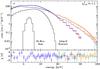 |
Fig. 4 a) Folded spectrum from epoch 6 together with best fit (red) and all model components, i.e., CutoffPL, 10 keV feature, Fe Kα fluorescence line, and five cyclotron features. b) Residuals of the best fit, shown as the difference between the data and the model normalized to the uncertainty of each data point. Dark blue data points correspond to PCA, cyan points to HEXTE, and orange points to ISGRI. |
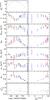 |
Fig. 5 Left temporal evolution and right luminosity dependence of the continuum parameters (see text for definitions) and 10 keV feature for the fits with the CutoffPL continuum. The color gradient from reddish to blueish data points indicates the temporal evolution of the outburst. The data points show results from the initial fit run, where a variable number of cyclotron lines was used. Green data points in the left column correspond to the second fit run with a fixed number of three cyclotron lines (only in the left column), which was been performed as a consistency check (see text for details). Where no green points are visible, both fits gave the same results. LX is in units of 1037 erg s-1. AG and AFe are in units of photons s-1 cm-2, while AFe is in multiples of 10-3. |
The two fit runs show that almost all fit parameters are equal within their respective uncertainties for both runs. Only Efold and the line parameters of the second harmonic are slightly different in epoch 6 and 7. These differences can be explained by the fact that for these two cases the second run has to account for the equivalent of the four harmonics required in the first run. The differences affect mainly the higher energies and are compensated by a change in the folding energy and the closest cyclotron line, i.e., the second harmonic. The remainder of this paper is based on the results from the first fit run.
An example for the best fit using the CutoffPL continuum with 10 keV feature and five cyclotron features (first fit run, epoch 6) is shown together with all model components in Fig. 4. This spectrum was recorded by all three instruments during the maximum of the outburst, i.e., epoch 6. All fit results from runs using the CutoffPL continuum are summarized in Table 2.
Continuum parameters of the time resolved spectral analysis.
4. Spectral evolution: No anticorrelation of the cyclotron line energy with flux
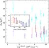 |
Fig. 6 Luminosity and time dependence (inset) of the energy of the fundamental CRSF using the CutoffPL continuum model. The color coding is the same as in Fig. 5. Cyan data points (diamonds) show the results when using the NPEX continuum. |
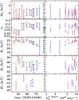 |
Fig. 7 Time (left) and luminosity (right) dependence of the parameters of the CRSF. The color coding is the same as in Fig. 5. |
Figures 5–7 show the evolution of the continuum and cyclotron line parameters as well as the parameters for the Fe Kα line for the first fit run with the CutoffPL continuum and 10 keV feature, and fixed NH (see also Table 2). As already noted in previous analyses for 4U 0115+634, the continuum varies over the outburst (e.g., Li et al. 2012). During the brightest phases of the outburst the spectrum is the hardest one. As shown in Fig. 3, the variation of Γ is significantly larger than the very slight correlation seen between Γ and Efold. As expected, the source’s intrinsic iron Kα line is significantly present during all epochs. As also observed in other X-ray transient pulsars (Inoue 1985) and expected for a line originating from fluorescence, the line flux is positively correlated to the X-ray flux from the source. The equivalent width stays constant within the uncertainties over the outburst. The 10 keV feature varies in both, the centroid energy EG and its flux AG. Its energy seems to be slightly anticorrelated with the source flux, while the relative flux in the feature, i.e., the ratio between the flux in the 10 keV feature and the total flux, remains constant. Its width, σG, remains relatively constant between 3.0 keV and 3.5 keV.
Very different from virtually all previous analyses, however, the cyclotron line is seen to be only slightly varying over the outburst. The colored data points in Figs. 6 and 7 show the centroid energy, E0, the width, W0, and the optical depth, τ0, of the fundamental cyclotron line against time and flux for the CutoffPL continuum, modified with the 10 keV feature. In these fits, the width W0 remains constant throughout the outburst, and there is only a slight (~3σ) indication that the optical depth τ0 was somewhat shallower during the initial phases of the outburst, before ~MJD 54 552, although it cannot be excluded that some of this effect is due to a correlation with the “10 keV feature”, which during this time of the outburst peaks close to the cyclotron line at around 8 keV. Most importantly, however, as shown in Fig. 6 the energy of the fundamental cyclotron line is only very slightly variable: during early phases of the outburst the line is around 11 keV, moving towards 10 keV as the outburst progressed. This result is contrary to all earlier studies of outbursts of 4U 0115+634, where strong changes in the line energy were seen (e.g., Li et al. 2012; Tsygankov et al. 2007; Nakajima et al. 2006; Mihara et al. 2004).
Where does this difference in line behavior come from? As discussed in Sect. 3.1 a large variety of continuum models can be used to describe the broad band spectra of accreting neutron stars. Due to the early successes of fitting spectra of 4U 0115+634 with the NPEX and PLCUT models, these continua have been extensively used when modeling the outburst behavior of this pulsar. Unfortunately, however, in most previous analyses – including some of our own – no attempt was made at modeling the data with any of the other available models.
As an example, modeling the 2008 outburst of 4U 0115+634 with the NPEX model (following Nakajima et al. 2006, fixing Γ2 to 2.0) results in fits that are of only slight worse quality as those using the CutoffPL model modified by the 10 keV feature, and we can recover the strong variation of the cyclotron line found in earlier analyses (Fig. 6, cyan data points)4. Depending on the choice of the continuum, we therefore find a fundamentally different behavior of the fundamental cyclotron line, especially the centroid energy.
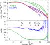 |
Fig. 8 a) PCA, HEXTE, and ISGRI spectra from epoch 9 (red) together with the best fit models using the NPEX (green) and CutoffPL (blue) continua after setting the optical depth of the cyclotron lines to zero. b) Ratio between the data and the model. |
Given that the fits with NPEX and CutoffPL give similarly good results, what is the fundamental difference between both modeling approaches? NPEX models generally result in very broad cyclotron lines, with W0 and W1 often exceeding 5 keV (e.g., Nakajima et al. 2006, runs using the PLCUT model give similar results, see, e.g., Li et al. 2012). In contrast, using the CutoffPL continuum with the 10 keV feature results in widths of typically less than 3 keV, much more consistent with the narrow shapes of the residuals shown in Fig. 2. When lines are as broad as in the NPEX fits, they can influence the continuum fit. To illustrate how strongly these features actually distort the continuum, Fig. 8 shows the continuum shape inferred when setting τ0, τ1, τ2, and τ3 to zero. The residuals for the CutoffPL continuum with the 10 keV feature (dark blue) show sharp absorption dips at the cyclotron line energies of the fundamental and first harmonic line energies. For the NPEX model (green line), on the other hand, it is obvious that rather than describing narrow cyclotron lines, the multiplicative broad line model strongly influences the continuum. As discussed above, our spectral fits show that during the brightest phases of the outburst a significant hardening of the continuum emission is observed, together with a change of the exponential cutoff. While this is also seen in the variation of the continuum parameters, it is very likely that the luminosity dependence of the CRSF in the NPEX fits is due to the line partially modeling this behavior of the continuum, and not a real physical effect.
Using the results from the CutoffPL plus 10 keV feature fits for the line energy also solves another problem found in earlier spectral modeling. Here, using NPEX fits, the ratios between the fundamental and higher cyclotron lines were often found to deviate significantly from integers. While slightly non-integer ratios are expected when taking relativistic quantum mechanics into account (see the discussion by Pottschmidt et al. 2005), the large deviations from integer multiples seen previously (e.g., Tsygankov et al. 2007; Nakajima et al. 2006; Heindl et al. 1999; Santangelo et al. 1999) require rather complex model assumptions which introduce second order effects such as strong vertical B-field gradients, crustal field structures on small scales, or thermomagnetic effects for their explanation (see Schönherr et al. 2007, and references therein for a discussion). Figure 9 shows that we can recover these non-integer ratios in our NPEX fits, but when using the CutoffPL plus 10 keV feature model, these ratios are mostly in agreement with integer values, or at least only slightly higher, as expected from the most simple models for cyclotron line formation. We conclude that also from a physical point of view, the CutoffPL continuum with the 10 keV feature gives a much more satisfactory description of the data.
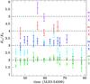 |
Fig. 9 Ratios of the cyclotron line energies En/E0 with respect to the centroid energy of the fundamental line against time. The dark green, dark blue, red and purple data points (bars) correspond to E1/E0, E2/E0, E3/E0, and E4/E0, respectively, using the CutoffPL continuum with a 10 keV feature. The light green and cyan data points (filled circles) show the results for E1/E0 and E2/E0 using NPEX. The dashed lines indicate integer values for these ratios. |
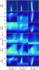 |
Fig. 10 Confidence contours between the fundamental CRSF energy and other fit parameters. The columns show the results for epochs 2, 6, and 14, respectively. Contour lines correspond to the 68.3%, 90%, and 99% confidence level. Color indicates Δχ2 with respect to the best fit value, with the color scale running from orange (low Δχ2) to dark blue (large Δχ2). |
Finally, we check the dependence of the line position on other free fit parameters when using the CutoffPL continuum modified by the 10 keV feature. Since the origin of the 10 keV feature remains still an open questtion, possible relations between the CRSF centroid energy and the parameters of the 10 keV feature have to be investigated, and other continuum parameters such as Efold or Γ could influence the results for the cylotron line parameters. Figure 10 shows the behavior of Δχ2 in the vicinity of the best fit values for three epochs representative for the early phase, peak, and late phase of the 2008 outburst for selected combinations of important fit parameters. These contour plots show that the line energy is not affected by cross correlations with other parameters, i.e., possible variations in the line energy of the fundamental cyclotron line are not due to variations observed in the parameters of the 10 keV feature or the continuum parameters.
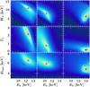 |
Fig. 11 Confidence contours between the fundamental cyclotron line energy and continuum parameters when using the NPEX model. The displayed epochs, colors and lines are the same as in Fig. 10. |
In contrast to the stable behavior of the line when using CutoffPL with a 10 keV feature, Fig. 11 illustrates the dependence of the CRSF centroid energy on the continuum parameters of the NPEX model. In many cases, strong correlations between E0 and Γ1 as well as between E0 and Efold are present. These correlations are a further indicator that the Lorentzian component is used to model the continuum rather than a cyclotron line when using the NPEX model.
5. Summary and conclusion
In this paper we have presented a study of the 2008 outburst of 4U 0115+634 based on RXTE and INTEGRAL data (Fig. 1). We reproduced the results from previous work (e.g., Nakajima et al. 2006; Tsygankov et al. 2007; Li et al. 2012, and others), that the spectra can be successfully modeled by, e.g., the NPEX model. We showed that for these fits the very broad absorption features, which are thought to describe the CRSFs, rather model the broadband continuum. Our result that the continuum parameters are strongly variable over the outburst (Fig. 5), could be responsible for the change in the cyclotron line energy in these fits.
We have shown that the spectral continuum can be also well described with a model introduced by Klochkov et al. (2007) for EXO 2030+375 and Ferrigno et al. (2009) for 4U 0115+634, i.e., the CutoffPL, modified by strong Gaussian emission feature around 10 keV and several (up to five) cyclotron lines (Table 2 and Fig. 4). Due to an unphysical break close to the energy of the fundamental cyclotron line, the PLCUT model does not give a physical description of the continuum. Using the CutoffPL together with the 10 keV feature, we have shown that the modeling of lines reflects the theoretical expectation in both the line shape and the ratios of the harmonics. In this model, the luminosity dependency of the centroid energy is not present. As shown also by Ferrigno et al. (2011), the line centroid energy is remarkably stable throughout the brightest phase of the outburst. Here we show that such stability is present, albeit at lower significance, also during the early and late phases. In this model, the continuum variations are explained by a slight anticorrelation of the centroid energy of the Gaussian feature with luminosity and a significant variation of Γ.
The strong systematic influence of the chosen continuum on the cyclotron line behavior illustrates a problem that is potentially inherent to all cyclotron line measurements. We emphasize, however, that this does not mean that the general picture of the different regimes of magnetized neutron star accretion and general luminosity dependence of the cyclotron line as outlined by Becker et al. (2012, and references therein) is incorrect. In the sample of sources discussed by Becker et al. (2012), 4U 0115+634 was an outlier. The change of line energy inferred from the NPEX and PLCUT models was almost a jump at a 3–50 keV luminosity of around 3 × 1037 erg s-1 and strong hysteresis effects were present (Fig. 6). Such a behavior has not been seen in any of the other cyclotron line sources. The second strongest luminosity-dependent cyclotron line variability is observed in V0332+53 (Mowlavi et al. 2006; Tsygankov et al. 2006; Nakajima et al. 2010), in which the cyclotron lines are so strong that the change can be seen by eye even in the raw detector spectra. While the boundaries between the different accretion regimes estimated by Becker et al. (2012) might therefore have to be adjusted, the overall principal behavior of the accretion column discussed by these authors still holds.
With the recently successful launch of NuSTAR (Harrison et al. 2010), a low background, focusing telescope with slightly higher resolution than the RXTE-HEXTE or the Suzaku-HXD is now available. With its higher resolution and the much higher expected signal to noise ratio in the spectra, we will be able, for the first time, to resolve cyclotron lines and study their luminosity-dependent behavior without the danger of a systematic influence of the choice of a continuum.
Often one fixes Γ2 = 2, see, e.g., Nakajima et al. (2006).
Modeling the spectra with the PLCUT model results in an unphysical break around the energy of the fundamental line, we therefore consider this continuum to be unsuitable for studying the cyclotron line behavior.
Acknowledgments
We thank the referee for his/her insightful comments. We also thank the schedulers of RXTE and INTEGRAL for their role in making this campaign possible, and the International Space Science Institute in Bern, Switzerland, for their hospitality. We acknowledge funding by the Bundesministerium für Wirtschaft und Technologie under Deutsches Zentrum für Luft- und Raumfahrt grants 50OR0808, 50OR0905, and 50OR1113, and by the Deutscher Akademischer Austauschdienst. M.T.W. is supported by the US Office of Naval Research. IC acknowledges financial support from the French Space Agency CNES through CNRS. S.M.N. and J.M.T. acknowledge support from the Spanish Ministerio de Ciencia, Tecnología e Innovación (MCINN) through grant AYA2010-15431 and the use of the computer facilities made available through the grant AIB2010DE-00057. This research is in part based on observations with INTEGRAL, an ESA project with instruments and science data centre funded by ESA member states (especially the PI countries: Denmark, France, Germany, Italy, Switzerland, Spain), Czech Republic, and Poland, and with the participation of Russia and USA. We thank John E. Davis for the development of the SLxfig module, which was used to create all figures in the paper.
References
- Arnaud, K. A. 1996, in Astronomical Data Analysis Software and Systems V, eds. J. H. Jacoby, & J. Barnes, (San Francisco: Astron. Soc. Pacific), ASP Conf. Ser., 101, 17 [Google Scholar]
- Basko, M. M., & Sunyaev, R. A. 1976, MNRAS, 175, 395 [NASA ADS] [CrossRef] [Google Scholar]
- Becker, P. A., & Wolff, M. T. 2007, ApJ, 654, 435 [NASA ADS] [CrossRef] [Google Scholar]
- Becker, P. A., Klochkov, D., Schönherr, G., et al. 2012, A&A, 544, A123 [NASA ADS] [CrossRef] [EDP Sciences] [Google Scholar]
- Bradt, H. V., Rothschild, R. E., & Swank, J. H. 1993, A&AS, 97, 355 [NASA ADS] [Google Scholar]
- Burnard, D. J., Arons, J., & Klein, R. I. 1991, ApJ, 367, 575 [CrossRef] [Google Scholar]
- Caballero, I., & Wilms, J. 2011, Mem. Soc. Astron. It., 83, 230 [Google Scholar]
- Caballero, I., Kretschmar, P., Santangelo, A., et al. 2007, A&A, 465, L21 [NASA ADS] [CrossRef] [EDP Sciences] [Google Scholar]
- Coburn, W. 2001, Ph.D. Thesis, University of California, San Diego [Google Scholar]
- Cominsky, L., Clark, G. W., Li, F., Mayer, W., & Rappaport, S. 1978, Nature, 273, 367 [NASA ADS] [CrossRef] [Google Scholar]
- Davidson, K. 1973, Nature, 246, 1 [NASA ADS] [CrossRef] [Google Scholar]
- Ferrigno, C., Becker, P. A., Segreto, A., Mineo, T., & Santangelo, A. 2009, A&A, 498, 825 [NASA ADS] [CrossRef] [EDP Sciences] [Google Scholar]
- Ferrigno, C., Falanga, M., Bozzo, E., et al. 2011, A&A, 532, A76 [NASA ADS] [CrossRef] [EDP Sciences] [Google Scholar]
- Giacconi, R., Murray, S., Gursky, H., et al. 1972, ApJ, 178, 281 [NASA ADS] [CrossRef] [Google Scholar]
- Harrison, F. A., Boggs, S., Christensen, F., et al. 2010, in Space Telescopes and Instrumentation 2010: Ultraviolet to Gamma Ray, eds. M. Arnaud, S. S. Murray, & T. Takahashi, SPIE Conf. Ser., 7732, 77320 [Google Scholar]
- Heindl, W. A., Coburn, W., Gruber, D. E., et al. 1999, ApJ, 521, L49 [NASA ADS] [CrossRef] [Google Scholar]
- Heindl, W. A., Coburn, W., Gruber, D. E., et al. 2000, in The Fifth Compton Symposium, eds. M. L. McConnell, & J. M. Ryan, AIP Conf. Ser., 510, 173 [Google Scholar]
- Houck, J. C., & Denicola, L. A. 2000, in Astronomical Data Analysis Software and Systems IX, eds. N. Manset, C. Veillet, & D. Crabtree, ASP Conf. Ser. 216, 591 [Google Scholar]
- Inoue, H. 1985, Space Sci. Rev., 40, 317 [NASA ADS] [CrossRef] [Google Scholar]
- Jahoda, K., Markwardt, C. B., Radeva, Y., et al. 2006, ApJS, 163, 401 [NASA ADS] [CrossRef] [Google Scholar]
- Johns, M., Koski, A., Canizares, C., et al. 1978, IAU Circ., 3171 [Google Scholar]
- Klochkov, D., Horns, D., Santangelo, A., et al. 2007, A&A, 464, L45 [NASA ADS] [CrossRef] [EDP Sciences] [Google Scholar]
- Klochkov, D., Santangelo, A., Staubert, R., & Ferrigno, C. 2008, A&A, 491, 833 [NASA ADS] [CrossRef] [EDP Sciences] [Google Scholar]
- Klochkov, D., Staubert, R., Santangelo, A., Rothschild, R. E., & Ferrigno, C. 2011, A&A, 532, A126 [NASA ADS] [CrossRef] [EDP Sciences] [Google Scholar]
- Kretschmar, P., Kreykenbohm, I., Wilms, J., et al. 1997, in The Transparent Universe, eds. C., Winkler, T. J.-L., Courvoisier, & P., Durouchoux, ESA SP, 382, 141 [Google Scholar]
- Kreykenbohm, I., Kretschmar, P., Wilms, J., et al. 1999, A&A, 341, L141 [NASA ADS] [Google Scholar]
- Kreykenbohm, I., Coburn, W., Wilms, J., et al. 2002, A&A, 395, 129 [NASA ADS] [CrossRef] [EDP Sciences] [Google Scholar]
- Krimm, H. A., Barthelmy, S. D., Baumgartner, W., et al. 2008, Astron. Tel., 1427 [Google Scholar]
- Lebrun, F., Leray, J. P., Lavocat, P., et al. 2003, A&A, 411, 141 [Google Scholar]
- Li, J., Wang, W., & Zhao, Y. 2012, MNRAS, 423, 2854 [NASA ADS] [CrossRef] [Google Scholar]
- Makishima, K., Mihara, T., Nagase, F., & Tanaka, Y. 1999, ApJ, 525, 978 [NASA ADS] [CrossRef] [Google Scholar]
- Mészáros, P. 1984, Space Sci. Rev., 38, 325 [NASA ADS] [CrossRef] [Google Scholar]
- Mészáros, P. 1992, High-energy radiation from magnetized neutron stars (Chicago: Chicago Univ. Press) [Google Scholar]
- Mihara, T., Makishima, K., Ohashi, T., Sakao, T., & Tashiro, M. 1990, Nature, 346, 250 [NASA ADS] [CrossRef] [Google Scholar]
- Mihara, T., Makishima, K., & Nagase, F. 2004, ApJ, 610, 390 [NASA ADS] [CrossRef] [Google Scholar]
- Mowlavi, N., Kreykenbohm, I., Shaw, S., et al. 2006, A&A, 451, 817 [NASA ADS] [CrossRef] [EDP Sciences] [Google Scholar]
- Müller, S., Obst, M., Kreykenbohm, I., et al. 2010, in Proc. Eighth Integral Workshop. The Restless Gamma-ray Universe (INTEGRAL 2010), PoS(INTEGRAL 2010)116 [Google Scholar]
- Nagase, F., Dotani, T., Tanaka, Y., et al. 1991, ApJ, 375, L49 [NASA ADS] [CrossRef] [Google Scholar]
- Nakajima, M., Mihara, T., Makishima, K., & Niko, H. 2006, ApJ, 646, 1125 [NASA ADS] [CrossRef] [Google Scholar]
- Nakajima, M., Mihara, T., & Makishima, K. 2010, ApJ, 710, 1755 [NASA ADS] [CrossRef] [Google Scholar]
- Negueruela, I., & Okazaki, A. T. 2001, A&A, 369, 108 [NASA ADS] [CrossRef] [EDP Sciences] [Google Scholar]
- Pottschmidt, K., Kreykenbohm, I., Wilms, J., et al. 2005, ApJ, 634, L97 [NASA ADS] [CrossRef] [Google Scholar]
- Rappaport, S., Clark, G. W., Cominsky, L., Li, F., & Joss, P. C. 1978, ApJ, 224, 1 [NASA ADS] [CrossRef] [Google Scholar]
- Rothschild, R. E., Blanco, P. R., Gruber, D. E., et al. 1998, ApJ, 496, 538 [NASA ADS] [CrossRef] [Google Scholar]
- Rothschild, R. E., Markowitz, A., Rivers, E., et al. 2011, ApJ, 733, 23 [NASA ADS] [CrossRef] [Google Scholar]
- Santangelo, A., Segreto, A., Giarrusso, S., et al. 1999, ApJ, 523, L85 [NASA ADS] [CrossRef] [Google Scholar]
- Schönherr, G., Wilms, J., Kretschmar, P., et al. 2007, A&A, 472, 353 [NASA ADS] [CrossRef] [EDP Sciences] [Google Scholar]
- Staubert, R., Shakura, N. I., Postnov, K., et al. 2007, A&A, 465, L25 [NASA ADS] [CrossRef] [EDP Sciences] [Google Scholar]
- Tanaka, Y. 1986, in Radiation Hydrodynamics in Stars and Compact Objects, eds. D., Mihalas, & K. H., Winkler (New York: Springer), IAU Coll., 86, 198 [Google Scholar]
- Torrejón, J. M., Schulz, N. S., Nowak, M. A., & Kallman, T. R. 2010, ApJ, 715, 947 [NASA ADS] [CrossRef] [Google Scholar]
- Tsygankov, S. S., Lutovinov, A. A., Churazov, E. M., & Sunyaev, R. A. 2006, MNRAS, 371, 19 [NASA ADS] [CrossRef] [Google Scholar]
- Tsygankov, S. S., Lutovinov, A. A., Churazov, E. M., & Sunyaev, R. A. 2007, Astron. Lett., 33, 368 [NASA ADS] [CrossRef] [Google Scholar]
- Unger, S. J., Roche, P., Negueruela, I., et al. 1998, A&A, 336, 960 [NASA ADS] [Google Scholar]
- Verner, D. A., & Yakovlev, D. G. 1995, A&AS, 109, 125 [NASA ADS] [Google Scholar]
- Wheaton, W. A., Doty, J. P., Primini, F. A., et al. 1979, Nature, 282, 240 [NASA ADS] [CrossRef] [Google Scholar]
- White, N. E., Swank, J. H., & Holt, S. S. 1983, ApJ, 270, 711 [NASA ADS] [CrossRef] [Google Scholar]
- Wilms, J., Allen, A., & McCray, R. 2000, ApJ, 542, 914 [NASA ADS] [CrossRef] [Google Scholar]
- Winkler, C., Courvoisier, T. J.-L., Di Cocco, G., et al. 2003, A&A, 411, L1 [NASA ADS] [CrossRef] [EDP Sciences] [Google Scholar]
All Tables
All Figures
|
Fig. 1 RXTE/ASM lightcurve of 4U 0115+634 (2–12 keV). The inset shows a close-up view of this lightcurve, showing the 2008 outburst in detail. Arrows indicate the times of pointed RXTE and INTEGRAL observations. Numbers indicate the observation epochs used in the data analysis (see also Table 1). |
| In the text | |
|
Fig. 2 Deviations between the data and the best fit with CutoffPL and 10 keV feature for the PCA (circles), HEXTE (crosses), and ISGRI (filled diamonds) in units of standard deviations σ. For these fits, no cyclotron lines have been taken into account. The numbers on the right side indicate the respective epoch. |
| In the text | |
|
Fig. 3 a) c) and d) Confidence contours for the folding energy, the photon index and the hydrogen column density for epoch 6. b) Confidence contours between the Efold and Γ with NH frozen to 1.7 × 1022 cm-2. Contour lines correspond to the 68.3%, 90%, and 99% level. Color indicates Δχ2 with respect to the best fit value, with the color scale running from orange (low Δχ2) to dark blue (large Δχ2). |
| In the text | |
|
Fig. 4 a) Folded spectrum from epoch 6 together with best fit (red) and all model components, i.e., CutoffPL, 10 keV feature, Fe Kα fluorescence line, and five cyclotron features. b) Residuals of the best fit, shown as the difference between the data and the model normalized to the uncertainty of each data point. Dark blue data points correspond to PCA, cyan points to HEXTE, and orange points to ISGRI. |
| In the text | |
|
Fig. 5 Left temporal evolution and right luminosity dependence of the continuum parameters (see text for definitions) and 10 keV feature for the fits with the CutoffPL continuum. The color gradient from reddish to blueish data points indicates the temporal evolution of the outburst. The data points show results from the initial fit run, where a variable number of cyclotron lines was used. Green data points in the left column correspond to the second fit run with a fixed number of three cyclotron lines (only in the left column), which was been performed as a consistency check (see text for details). Where no green points are visible, both fits gave the same results. LX is in units of 1037 erg s-1. AG and AFe are in units of photons s-1 cm-2, while AFe is in multiples of 10-3. |
| In the text | |
|
Fig. 6 Luminosity and time dependence (inset) of the energy of the fundamental CRSF using the CutoffPL continuum model. The color coding is the same as in Fig. 5. Cyan data points (diamonds) show the results when using the NPEX continuum. |
| In the text | |
|
Fig. 7 Time (left) and luminosity (right) dependence of the parameters of the CRSF. The color coding is the same as in Fig. 5. |
| In the text | |
|
Fig. 8 a) PCA, HEXTE, and ISGRI spectra from epoch 9 (red) together with the best fit models using the NPEX (green) and CutoffPL (blue) continua after setting the optical depth of the cyclotron lines to zero. b) Ratio between the data and the model. |
| In the text | |
|
Fig. 9 Ratios of the cyclotron line energies En/E0 with respect to the centroid energy of the fundamental line against time. The dark green, dark blue, red and purple data points (bars) correspond to E1/E0, E2/E0, E3/E0, and E4/E0, respectively, using the CutoffPL continuum with a 10 keV feature. The light green and cyan data points (filled circles) show the results for E1/E0 and E2/E0 using NPEX. The dashed lines indicate integer values for these ratios. |
| In the text | |
|
Fig. 10 Confidence contours between the fundamental CRSF energy and other fit parameters. The columns show the results for epochs 2, 6, and 14, respectively. Contour lines correspond to the 68.3%, 90%, and 99% confidence level. Color indicates Δχ2 with respect to the best fit value, with the color scale running from orange (low Δχ2) to dark blue (large Δχ2). |
| In the text | |
|
Fig. 11 Confidence contours between the fundamental cyclotron line energy and continuum parameters when using the NPEX model. The displayed epochs, colors and lines are the same as in Fig. 10. |
| In the text | |
Current usage metrics show cumulative count of Article Views (full-text article views including HTML views, PDF and ePub downloads, according to the available data) and Abstracts Views on Vision4Press platform.
Data correspond to usage on the plateform after 2015. The current usage metrics is available 48-96 hours after online publication and is updated daily on week days.
Initial download of the metrics may take a while.