| Issue |
A&A
Volume 550, February 2013
|
|
|---|---|---|
| Article Number | A135 | |
| Number of page(s) | 18 | |
| Section | Interstellar and circumstellar matter | |
| DOI | https://doi.org/10.1051/0004-6361/201220096 | |
| Published online | 07 February 2013 | |
The thermal state of molecular clouds in the Galactic center: evidence for non-photon-driven heating⋆,⋆⋆
1
Max-Planck-Institut für Radioastronomie,
Auf dem Hügel 69, 53121
Bonn,
Germany
e-mail:
This email address is being protected from spambots. You need JavaScript enabled to view it.
2
Purple Mountain Observatory, Chinese Academy of
Sciences, 210008
Nanjing, PR
China
3
Astron. Dept., King Abdulaziz University,
PO Box 80203, Jeddah, Saudi
Arabia
4
ESO, Karl-Schwarzschild Strasse 2, 85748
Garching bei München,
Germany
5
Joint ALMA Observatory, Av. Alonso de Córdova 3107, Vitacura,
Santiago,
Chile
6
Department of Earth and Space Sciences, Chalmers University of
Technology, Onsala Observatory, 439 94
Onsala,
Sweden
7
Argelander-Institut für Astronomie, Universität
Bonn, Auf dem Hügel
71, 53121
Bonn,
Germany
8
National Radio Astronomy Observatory, 520 Edgemont Rd., Charlottesville, VA, 22903, USA
Received:
24
July
2012
Accepted:
29
November
2012
Abstract
We used the Atacama Pathfinder Experiment (APEX) 12 m telescope to observe the JKAKc = 303 → 202, 322 → 221, and 321 → 220 transitions of para-H2CO at 218GHz simultaneously to determine kinetic temperatures of the dense gas in the central molecular zone (CMZ) of our Galaxy. The map extends over approximately 40′ × 8′ (~100 × 20pc2) along the Galactic plane with a linear resolution of 1.2pc. The strongest of the three lines, the H2CO (303 → 202) transition, is found to be widespread, and its emission shows a spatial distribution similar to ammonia. The relative abundance of para-H2CO is 0.5−1.2 × 10⁻⁹, which is consistent with results from lower frequency H2CO absorption lines. Derived gas kinetic temperatures for individual molecular clouds range from 50K to values in excess of 100K. While a systematic trend toward (decreasing) kinetic temperature versus (increasing) angular distance from the Galactic center (GC) is not found, the clouds with highest temperature (Tkin> 100K) are all located near the nucleus. For the molecular gas outside the dense clouds, the average kinetic temperature is 65 ± 10K. The high temperatures of molecular clouds on large scales in the GC region may be driven by turbulent energy dissipation and/or cosmic-rays instead of photons. Such a non-photon-driven thermal state of the molecular gas provides an excellent template for the more distant vigorous starbursts found in ultraluminous infrared galaxies (ULIRGs).
Key words: Galaxy: center / ISM: clouds / ISM: molecules / radio lines: ISM
Appendices are available in electronic form at http://www.aanda.org
Based on observations made with ESO telescopes at the La Silla Paranal Observatory under programme 085.B-0964.
© ESO, 2013
1. Introduction
The Galactic center (GC) region is the closest galaxy core. It is characterized by a high concentration of molecular gas located in the innermost few hundred parsec of the Milky Way, the central molecular zone (CMZ; Morris & Serabyn 1996), and by extreme conditions like high mass densities, large velocity dispersions, strong tidal forces, and strong magnetic fields. Therefore it is a unique laboratory for studying molecular gas in an environment that is quite different from that of the Milky Way’s disk. For a general understanding of the physics involved in galactic cores, measurements of basic physical parameters, such as molecular gas density and gas kinetic temperature, are indispensable.
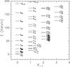 |
Fig. 1 H2CO energy-level diagram up to 200K. The H2CO 218GHz transitions observed in this paper are shown in bold. |
In local dark clouds, gas temperatures can be constrained by observations of the J=1 → 0 transition of CO, both because this transition is opaque and easily thermalized and because the emission even fills the beam of a single-dish telescope. At a distance of 8 kpc (Reid 1993), however, the beam filling factor of CO J=1 → 0 emission is unknown, and the GC clouds may also be affected by self-absorption. Analysis of multilevel studies of commonly observed linear molecules like CO, HCN, or HCO+ suffers from a coupled sensitivity to the kinetic temperature and gas density, making an observed line ratio consistent with both a high density at a low temperature and a low density at a high temperature. The metastable inversion lines of the symmetric top molecule ammonia (NH3) are frequently used as a galactic standard cloud thermometer (Walmsley & Ungerechts 1983; Danby et al. 1988). Radiative transitions between K-ladders of NH3 are forbidden, and therefore the relative populations1 depend on the kinetic temperature of the molecular gas rather than its density. However, the fractional abundance of NH3 varies between 10-5 in hot cores and 10-8 in dark clouds (e.g. Benson & Myers 1983; Mauersberger et al. 1987). Furthermore, NH3 is extremely affected by a high UV flux and tends to show a characteristic “concave” shape in rotation diagrams, either caused by a variety of layers with different temperatures (e.g., due to shocks) or by the specifics of the collision rates. Symmetric top molecules such as CH3C2H and CH3CN are not widespread and their emission is very faint (Bally et al. 1987; Nummelin et al. 1998). Therefore we should look for a widespread symmetric or slightly asymmetric top molecule that is more favorable for spectroscopic studies to derive the kinetic temperature of the entire molecular gas.
Formaldehyde (H2CO) is such a molecule. It is truly ubiquitous. Wootten et al. (1978) suggested that fractional H2CO abundances decrease with increasing density of the gas in star forming regions of the Galactic disk. However, this may be due instead to decreasing volume filling factors with increasing density (e.g., Mundy et al. 1987). Unlike for NH3, variations in the fractional abundance of H2CO rarely exceed one order of magnitude (Johnstone et al. 2003). To give an example: the H2CO abundance is the same in the hot core and in the compact ridge of the Orion nebula, whereas the NH3 hot core abundance surpasses that of the ridge by about two orders of magnitude (Caselli et al. 1993; Mangum et al. 1993). We also note that for the starburst galaxy M82, Tkin(NH3)~60K, while for the bulk of the molecular gas Tkin(H2CO)~200K (Weißet al. 2001; Mauersberger et al. 2003; Mühle et al. 2007).
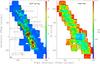 |
Fig. 2 H2CO (303 → 202) integrated intensity map (left)
and the noise map (right) observed with the APEX in the GC. Left:
black contour levels for the molecular line emission (on a
|
The relative populations of the Ka ladders of H2CO (see Fig. 1 for an energy level diagram) are almost exclusively determined by collisional processes (Mangum & Wootten 1993). Therefore, line ratios involving different Ka ladders of one of the subspecies, either ortho- or para-H2CO, are good tracers of the kinetic temperature (Mangum & Wootten 1993; Mühle et al. 2007). The energy levels above the ground (para)-H2CO state are 10.5 and 21.0K for the lower and upper states of H2CO (303 → 202), and 57.6 and 68.1K for H2CO (321 → 220) and (322 → 221) (see Fig. 1 for all H2CO energy levels under 200K). Therefore, the line ratios are sensitive to gas kinetic temperatures less than 100K, and the uncertainty in gas temperature is relatively small for a measured line ratio at Tkin<100K (also see Mangum & Wootten 1993) in the case of optically thin H2CO emission. At higher temperatures, the H2CO 218GHz transitions are less ideal because small changes in the ratios yield significant changes in Tkin, so that the H2CO J=5−4 transitions at ~364GHz are then becoming better tracers (Mangum & Wootten 1993). The JKAKc = 303 → 202, 322 → 221, and 321 → 220 transitions of para-H2CO stand out by being close in frequency. With rest frequencies of 218.222, 218.475, and 218.760GHz, respectively, all three lines can be measured simultaneously by employing a bandwidth of 1GHz. In this way, the inter-ladder line ratios H2CO 322 → 221/303 → 202 and 321 → 220/303 → 202, are free of uncertainties related to pointing accuracy, calibration errors, and different beam widths. In this paper, we therefore present observations of the H2CO line triplet at 218GHz to study the gas kinetic temperatures of Galactic center clouds.
2. Observations and data reduction
Simultaneous measurements of the JKAKc = 303 → 202, 322 → 221, and 321 → 220 transitions of para-H2CO (see Sect. 1 and Fig. 1) were obtained with the Atacama Pathfinder Experiment (APEX2, Güsten et al. 2006) 12 m telescope located on Chajnantor (Chile) between 2010 April and 2010 June. We used the APEX-1 receiver, operating at 211−270 GHz, which employs a superconductor-insulator-superconductor (SIS) mixer with a typical sideband rejection >10dB. As backends we used a fast fourier transform Spectrometer (FFTS, Klein et al. 2006), which consists of two units with a bandwidth of 1 GHz each and a channel separation of 244 kHz. The full-width-at-half-maximum (FWHM) beam size was approximately 30″ in the observed frequency range and the typical pointing error was ~3″. The main beam efficiency and the forward efficiency were 0.75 and 0.97, respectively.
We used the on-the-fly observing mode measuring 4′ × 4′ maps in steps of 9′′ in both right ascension and declination, 0.8s integration time per position, and one OFF position measurement after every two map rows, i.e., after about one minute of observing time. The surveyed area is 302 square arcmin and its dimension is roughly 40′ × 8′ along the Galactic plane. The total observing time was about 41 h.
The data were reduced with the CLASS software3. We first excluded data with a high noise level due to distorted baselines. The spectra were resampled in steps of 15″ and smoothed to a velocity resolution of 2 km s-1. The final maps comprise 4825 points, corresponding to 4825 spectra for each transition. To optimize signal-to-noise ratios (S/N) of integrated intensity and channel maps, we had to determine the valid velocity ranges for the spectra, especially for those cases where the lines were weak. To avoid noise from channels without significant emission, we first created a high S/N spectrum by smoothing all spectra within a 60″ × 60″ box to obtain a masking spectrum, for which 1 and 0 were assigned for the channels with S/N higher and lower than 5, respectively. Different line windows were automatically deteremined to cover the emission from different positions, and the baseline was removed before creating the masking spectrum. Then, the final spectra were created by multiplying the raw spectrum by the masking spectrum. Because all lines were observed simultaneously and because the H2CO (303 → 202) data have the best S/N, the masking spectrum from this data set has also been applied to the other transitions by assuming the same velocity ranges for the emission from these transitions (for the details of this technique, see Dame et al. 2001; Dame 2011).
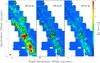 |
Fig. 3 Integrated intensity maps for the different transitions observed in the GC. The shown
region corresponds to the rectangle (black solid line) in Fig. 2 (left). Black contour levels for the molecular
line emission (on a |
3. Results
3.1. General characteristics of the molecular gas
For the first time, observations of the triple transitions of H2CO at 218GHz
have been performed in a large area of the GC. Fig. 2
(left panel) shows the extended line emission from the H2CO
(303 → 202) transition. Molecular gas, revealed by H2CO
(303 → 202), shows a similar spatial distribution as ammonia
(Güsten et al. 1981). All prominent features
identified in ammonia, e.g., the clouds M-0.13−0.08 and M-0.02−0.07 (the molecular clouds
labeled with M followed by the galactic coordinates are identified by Güsten et al. 1981), are clearly detected in H2CO
(303 → 202), and labeled in the figure. A map providing the noise
level of the full region is also presented in Fig. 2
(right panel). The median noise value for the 4825 spectra is about 0.1 K
( ) at a
velocity resolution of 2 km s-1. In the regions of interest where the line
emission is strong, the noise level is ~0.08 K (). To show
the line emission in more detail, we also present integrated intensity maps (Fig. 3), as well as channel maps (see Sect. 3.3), for all transitions in a zoomed region in Fig.
2 (left panel). The distribution of the velocity
integrated line emission of the observed three transitions is quite similar except that
the weaker two H2CO transitions are not detected in some of the regions where
the 303 → 202 transition is still observed.
) at a
velocity resolution of 2 km s-1. In the regions of interest where the line
emission is strong, the noise level is ~0.08 K (). To show
the line emission in more detail, we also present integrated intensity maps (Fig. 3), as well as channel maps (see Sect. 3.3), for all transitions in a zoomed region in Fig.
2 (left panel). The distribution of the velocity
integrated line emission of the observed three transitions is quite similar except that
the weaker two H2CO transitions are not detected in some of the regions where
the 303 → 202 transition is still observed.
3.2. Individual spectral lines
Spectra from some positions of interest are shown in Fig. B.1 with overlaid Gaussian fit profiles, and their locations are marked in Fig.
2 (left panel). To achieve better S/N, we averaged
the spectra within a 30″ × 30″ area to create a new spectrum for each transition. All
transitions from a given position are presented in the same panel of Fig. B.1 but with different offsets along the
y-axis. For those positions with clear detections of H2CO
322 → 221 and 321 → 220, line parameters are
listed in Table A.1, where integrated intensity,
 , peak
main beam brightness temperature, Tmb, local standard of rest
(LSR) velocity, V, and FWHM line width,
ΔV1/2, were obtained from Gaussian
fits. In most cases, only one component is needed for the Gaussian fits except in the case
of H2CO (322 → 221). This line is displaced from the
CH3OH(422 → 312) transition by only 49 km
s-1, and we therefore have applied in this case two component Gaussian fits.
, peak
main beam brightness temperature, Tmb, local standard of rest
(LSR) velocity, V, and FWHM line width,
ΔV1/2, were obtained from Gaussian
fits. In most cases, only one component is needed for the Gaussian fits except in the case
of H2CO (322 → 221). This line is displaced from the
CH3OH(422 → 312) transition by only 49 km
s-1, and we therefore have applied in this case two component Gaussian fits.
In the central nuclear region, line emission is too weak to be detected with sufficient S/N, while H2CO (303 → 202) emission is detected southwest, ~3pc away from Sgr A∗, showing the broad weak line profile belonging to P5 (−60″, −45″) in Fig. B.1.
The line parameters obtained from Gaussian fits do not show many peculiarities when one inspects the central velocities and line widths in Table A.1, as well as the line profiles in Fig. B.1. Sometimes, however, there are two velocity components, e.g., at offset positions P9 (60″, 120″) and P12 (150″, 225″) with respect to the Galactic center, and the number of components for their Gaussian fits had to be doubled. In particular, for the 44 km s-1component of P12, the H2CO (322 → 221) integrated intensity seems to be significantly larger than that of H2CO (321 → 220), because the H2CO (322 → 221) transition is blended by the emission from CH3OH(422 → 312) at 218.440 GHz.
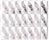 |
Fig. 4 Selected velocity-integrated maps for the different transitions observed in the GC.
Black contour levels for the molecular line emission (on a
|
3.3. Molecular line data cube
In Fig. 4, channel maps with velocity steps of 18 km s-1are presented, allowing us to clearly separate the components based on both their positions and velocities. The total integrated intensity maps are also shown for comparison in the panels on the righthand side. Channel maps in steps of 2 km s-1are presented in the Appendix (Figs. B.2−B.4) to show more detail.
We choose the H2CO (303 → 202) data to describe the individual molecular concentrations. H2CO 303 → 202 emission mainly ranges from −27 to 81 km s-1. In the velocity range [−27,−9], there are two prominent features, the −15 km s-1cloud M 0.02−0.05 at P12, and the southernmost cloud at P1. The latter is part of the 20 km s-1cloud M-0.13−0.08. There is also weak H2CO 303 → 202 emission at P5 close to Sgr A∗, which traces the southwestern lobe of the circumnuclear disk (CND).
Within the velocity range [−9,9], the bulk of the 20 km s-1cloud appears in the south and its size is about 7pc × 15pc. There are three small cores at P9, P11, and P12 with sizes of ~1 to 2pc in the northeast and one small cores at P17 even farther away from Sgr A∗. The peak of the 20 km s-1cloud moves from south (−75′′, −390′′) relative to the Galactic center to north (−30′′, −210′′), increasing the velocity from −27 to +27 km s-1.
Within the velocity range [9,27], there is a dense concentration at P7 with a size of ~2.7pc × 5.4pc. Extended weak emission is detected around P19 in an irregular morphology with a size of ~2pc × 9pc. The northernmost core, M 0.25+0.01, begins to appear at P22. This concentration is not fully covered by our observations.
In the velocity range [27,63], the line emission shows a complex morphology. The prominent features are the 50 km s-1cloud M-0.02−0.07 around P6, P7, and P8, two compact concentrations M 0.07−0.08 at P13 and M 0.11−0.08 at P15, an extended region of weak emission associated with M 0.06−0.04 around P12 and P14, a concentration M 0.10−0.01 around P16, and the northernmost core M 0.25+0.01 at P22. In the velocity range [27,45], the gas in the southeast close to Sgr A∗appears to connect the 20 km s-1and 50 km s-1clouds.
In the extreme velocity range [63,81], the 50 km s-1cloud moves to the west by ~60′′ with respect to [27,63], and peaks at P10, the edge of the cloud. In addition to features identified in the previous velocity ranges, there are three clumps around P18, P20, and P21, with sizes of about 3pc × 6pc.
4. Discussion
4.1. Formaldehyde column density and abundance
In the following we derive H2CO column densities and abundances. Assuming the
line emission is optically thin and the contribution from the cosmic microwave background
is negligible, the H2CO column density,
N(JKAKc),
in an upper state
JKAKc
can be obtained by 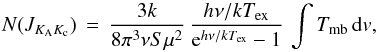 (1)(for the equations in
this subsection, see Mangum & Shirley 20084),
where h is Planck’s constant, k denotes Boltzmann’s
constant, μ is the dipole moment, ν the frequency of the
transition, Tex the excitation temperature, S
the line strength, Tmb the main beam brightness temperature,
and
(1)(for the equations in
this subsection, see Mangum & Shirley 20084),
where h is Planck’s constant, k denotes Boltzmann’s
constant, μ is the dipole moment, ν the frequency of the
transition, Tex the excitation temperature, S
the line strength, Tmb the main beam brightness temperature,
and  the
integrated line intensity for the transition
JKAKc → (J − 1)KAKc−1.
H2CO is a slightly asymmetric top molecule, and its line strength,
S, can be approximately calculated as for a symmetric top molecule by
the
integrated line intensity for the transition
JKAKc → (J − 1)KAKc−1.
H2CO is a slightly asymmetric top molecule, and its line strength,
S, can be approximately calculated as for a symmetric top molecule by
 (2)The total column
density, Ntotal, is related to the column density,
N(JKAKc),
in the upper state
JKAKc
by
(2)The total column
density, Ntotal, is related to the column density,
N(JKAKc),
in the upper state
JKAKc
by  (3)where
gJ(=2J + 1) is the rotational degeneracy,
gK marks the K degeneracy,
gI the nuclear spin degeneracy,
E(JKAKc)
the energy of state
JKAKc
above the ground level, and Z the partition function. The partition
function Z can be calculated by
(3)where
gJ(=2J + 1) is the rotational degeneracy,
gK marks the K degeneracy,
gI the nuclear spin degeneracy,
E(JKAKc)
the energy of state
JKAKc
above the ground level, and Z the partition function. The partition
function Z can be calculated by
 (4)For para-H2CO,
gK = 1, gI = 1,
and Ka can only be even. Here we include 41 levels with
energies above ground state up to 286K and assume the same excitation temperatures for all
transitions (i.e., local thermodynamical equilibrium, LTE) to estimate the partition
function. Substituting units and parameters for H2CO
(303 → 202)in Equation(3), and assuming an excitation temperature
of 10K, the total para-H2CO column density, Ntotal,
is
(4)For para-H2CO,
gK = 1, gI = 1,
and Ka can only be even. Here we include 41 levels with
energies above ground state up to 286K and assume the same excitation temperatures for all
transitions (i.e., local thermodynamical equilibrium, LTE) to estimate the partition
function. Substituting units and parameters for H2CO
(303 → 202)in Equation(3), and assuming an excitation temperature
of 10K, the total para-H2CO column density, Ntotal,
is 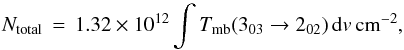 (5)where the integrated line
intensity,
(5)where the integrated line
intensity, 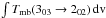 , is in units of K km
s-1.
, is in units of K km
s-1.
For the Sgr A∗complex with a size of 30pc in diameter, corresponding to ~13arcmin, the estimated molecular gas mass is ~0.4 × 10⁶M⊙(Kim et al. 2002), yielding an average H2 column density of 2.6 × 1022cm-2. In this region, 2161 formaldehyde spectra were obtained with a spacing of 15″, and the average spectrum has an integrated intensity of 10.5K km s-1on a Tmb scale. The derived averaged para-H2CO column density is 1.4 × 1013cm-2 assuming an excitation temperature of 10K. Adjusting the excitation temperature in the range of 5 to 40K, the resulting total para-H2CO column density will decrease with increasing Tex from 5K to around 14K, because with increasing Tex the populations of the J = 2 and 3 states become more dominant. Beyond Tex = 14K the resulting column densities will increase with excitation temperature because then also the J > 3 levels will be populated. For Tkin ≲ 100K (see Sect. 4.3 for large velocity gradient (LVG) modeling), Tex values ≳40K require densities ≳106cm-3, which are unrealistically high on a large spatial scale (e.g., Güsten & Henkel 1983). Therefore higher Tex values can probably be excluded and the corresponding averaged para-H2CO column density can be constrained to (1.3−3.1) × 1013cm-2. The resulting para-H2CO abundance is (0.5−1.2) × 10-9. This abundance agrees with the values found by Güsten & Henkel (1983) and Zylka et al. (1992), who used Ka=1 ortho-formaldehyde K-doublet absorption lines to obtain H2CO abundances of ~10-10 to 2 × 10⁻⁹ in the Galactic center region. Thus it is reasonable to adopt two fixed limiting para-H2CO abundances of 10-9 and 10-10 for the LVG analysis in Sect. 4.3.
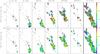 |
Fig. 5 H2CO 322 → 221/303 → 202 (top) and 321 → 220/303 → 202 (bottom) integrated intensity ratio map. Ratios are calculated when the H2CO 303 → 202 line emission is detected above 5σ. The top and bottom rows should be nearly identical, and the difference mainly comes from the CH3OH contamination in H2CO 322 → 221. The wedges at the sides show the line ratios. The beam size of 30″ is shown at the bottom-left corner. Sgr A∗ is the origin for the offset coordinates and shown as a cross. |
4.2. Line ratios
In this survey, the three 218GHz rotational transition lines of H2CO are observed simultaneously at the same angular resolution, providing good data sets to derive the H2CO line ratios. Before quantitatively determining gas kinetic temperatures, we first present H2CO 322 → 221/303 → 202 and 321 → 220/303 → 202 line ratios in Fig. 5 as probes of gas temperature. The line ratio maps are derived from both channel maps and total integrated intensity maps, and the ratios are calculated by integrating channels where the H2CO(303 → 202) line emission is detected above 5 σ. Since the excitation conditions for 322 → 221/303 → 202 and 321 → 220/303 → 202 are very similar, these two line ratio maps should be nearly identical, and indeed the differences mainly arise from the CH3OH contamination in H2CO 322 → 221.
As seen in Fig. 5, the H2CO 321 → 220/303 → 202 line ratio, with a median value of 0.23, varies significantly across the mapped region, from about 0.15 at the edge of the clouds to ~0.35 toward the 20 km s-1GMC and the compact concentration M 0.11−0.08 at P15. In case of narrow one-component features, the 322 → 221/303 → 202 ratios follow the same trend as the 321 → 220/303 → 202 ratios. For the 20 km s-1GMC, the line ratio is higher in the south than in the north in the velocity range [−9,9]. Within the velocity range [9,27], the ratio becomes higher at P3 in the north of the 20 km s-1GMC. The molecular clouds around P18, P19, and P20 have two velocity components as presented in Fig. B.1, one at ~25 km s-1and another at ~78 km s-1, and are characterized by low line ratios as clearly shown in Fig. 5(bottom). Higher line ratios tend to suggest higher gas kinetic temperatures and vice versa because the relative populations of the Ka ladders of H2CO are almost exclusively determined by collisional processes (Mangum & Wootten 1993). To be more quantitative and to relate the line ratios to kinetic temperatures, we need to adopt LVG radiative transfer modeling, which is done in the following section.
4.3. Kinetic temperatures of the Galactic center clouds
To evaluate gas kinetic temperatures, we selected the positions with the Gaussian fits listed in Table A.1 (see also Fig. B.1). To investigate the gas excitation from the H2CO line measurements, we use a one-component LVG radiative transfer model with collision rates from Green (1991) and choose a spherical cloud geometry with uniform kinetic temperature and density as described in Mangum & Wootten (1993). Dahmen et al. (1998) estimated that the velocity gradient ranges from 3 to 6km s-1 pc-1for Galactic center clouds. Here we adopt two fixed para-H2CO abundances of [para-H2CO] = 10-9 and 10-10 (see Sect. 4.1), and a velocity gradient of (dv/dr)=5 (km s-1)pc-1. The modeled parameter space encompasses gas temperatures, Tkin, from 10 to 300K with a step size of 5K and H2 number densities per cm3, lognH2, from 3.0 to 7.0 with a logarithmic step size of 0.1. According to Green (1991), collisional excitation rates for a given transition are accurate to ~20%.
We first choose the H2CO 322 → 221 and 303 → 202 data as input parameters. Although the 322 → 221 transition is blended with CH3OH at a few positions, its line emission is stronger than that of H2CO 321 → 220, and the components can be separated in all cases. This even holds for position P12 (see Sect. 3.2), where we have determined the central velocities of the two velocity components from H2CO 303 → 202 to then carry out a four-component Gaussian fit to both H2CO 303 → 202 and CH3OH 422 → 312. Comparing computed line intensities and their line ratios with the corresponding observational results, we can constrain the kinetic temperature. The gas density is not well known because it is highly dependent on the adopted fractional abundance, velocity gradient, and filling factors. Here we choose a filling factor of unity to fit the data, implying that we obtain beam averaged quantities.
 |
Fig. 6 Example of LVG modeling for P4. Top: reduced χ2 distribution (mainly vertical contours) for a single-component LVG model fit to the H2CO brightness temperatures (black contours, χ2=1,2,4), as well as H2CO 322 → 221/303 → 202 line ratios (mainly horizonal contours) as a function of nH2 and Tkin. The solid lines represent the line ratios: 0.05, 0.1, 0.15, 0.2, 0.25, 0.3, 0.35, 0.4. The red dashed lines show the observed line ratio and its lower and upper limits. The para-H2CO abundances per velocity gradient, [para-H2CO]/(dv/dr), for the LVG models are 2 × 10⁻¹⁰ pc(km s-1)-1 (left) and 2 × 10-11pc(km s-1)-1 (right), respectively. In the left panel the lines with a given H2CO line ratio move downwards (lower Tkin) at high density because the H2CO lines start to become saturated; this causes intensity ratios for a given Tkin to get closer to unity. Bottom: reduced χ2 distribution for the H2CO 321 → 220/303 → 202 line ratios. The kinetic temperature is sensitive to the gas density so this line ratio is a less suitable thermometer. |
H2CO LVG results.
In Fig. 6 (top), an example is presented to show how the parameters are constrained by the reduced χ2 distribution of H2CO line measurements in the Tkin-n parameter space. As can be seen, observed H2CO 322 → 221/303 → 202 line ratios (the approximately horizontal lines in the diagram) are a good measure of Tkin, independent of density, as long as the transitions are optically thin. In contrast, the density is poorly constrained, as can be inferred by the different resulting densities for the chosen limiting fractional H2CO abundances (in the specified case of Fig. 6, the range covers a factor of 3−4 if assuming a filling factor of unity). In Table 1, we present derived gas kinetic temperatures averaged over 30″ boxes at the positions shown in Figs. 2 and B.1. It is worth noting that in most cases the two adopted para-H2CO abundances, differing by a factor of 10 (Sect. 4.1), cause only a slight change of less than 10K in kinetic temperature because the 218GHz H2CO transitions remain optically thin in most parameter ranges except for gas densities higher than 104.6cm-3 in the case of [para-H2CO] = 10-9. For [para-H2CO] = 10-10 this limiting density is well above 105 and outside the plotted range of densities of Fig. 6 (top). This demonstrates that H2CO is a good molecular thermometer and can be used to reliably determine kinetic temperatures.
Gas temperatures range from 50 K in the southern part of the 20 km s-1cloud to
above 100 K in the 50 km s-1cloud and the molecular core of M 0.07−0.08. While
a systematic trend of (decreasing) kinetic temperature versus (increasing) angular
distance from the nucleus is not found, the clouds with highest temperature
(Tkin> 100K) are all located near
the center. To estimate the overall gas temperature on a large scale of ~90pc, we mask the
dense clouds by clipping all the emission above 3σ in
of the
H2CO (303 → 202) line within a 60″ × 60″ box and create
an averaged spectrum, yielding a gas kinetic temperature of 65 ± 10K for more diffuse
molecular gas outside of the dense cores in the GC region.
If we instead use the H2CO 321 → 220/303 → 202 line ratio to constrain gas properties, the kinetic temperature is somewhat more sensitive to the gas density so that this line ratio is not quite as good as a thermometer (see Fig. 6, bottom). Therefore, we focus exclusively on the H2CO 322 → 221/303 → 202 line ratio to derive the gas kinetic temperature in this study.
High gas temperatures were first deduced from the metastable transitions of ammonia (Güsten et al. 1981, 1985a,b; Hüttemeister et al. 1993). Using the CO 7−6/4−3 line ratio, Kim et al. (2002) report, for the Sgr A complex, a gas kinetic temperature of 47 K on a linear scale of 30pc. From mm- and submm-line spectroscopy, Oka et al. (2011) deduced temperatures of at least 63K in the CND. The 20 km s-1and 50 km s-1clouds were studied by Güsten et al. (1981, 1985a,b) with species like NH3 and CH3CN and by Mauersberger et al. (1986) in the (J,K)=(7,7) metastable inversion line of ammonia, yielding gas temperatures in the range 80−100 K. These results are roughly consistent with the temperatures derived by us from H2CO. We emphasize, however, that ammonia may be more affected than H2CO by a peculiar molecule specific chemistry and that the degeneracy between high Tkin and low n(H2) or vice versa is difficult to overcome for the mm- and submm-transitions from linear molecules.
A high gas temperature will affect the Jeans masses of dense cores (e.g., for a molecular
cloud, its Jeans’ mass is
MJ=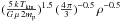 =
= M⊙,
where n is volume density and Tkin is gas
kinetic temperature. MJ ~1.2M⊙for
Tkin=10K and
n=105cm-3, and
14−39M⊙for Tkin=50−100K and
n=105cm-3), and may affect the initial mass
function (IMF) of star formation, resulting in a top-heavy IMF in the Galactic center
region (Klessen et al. 2007). Indeed, Alexander et
al. (2007) suggest a top-heavy IMF to explain the
observed ring of massive stars orbiting about 0.1 pc around the Galactic center. However,
Bartko et al. (2010) do not find evidence of a
top-heavy IMF at distances beyond 12″ from Sgr A∗. Higher densities in the GC
clouds with respect to those in the spiral arms due to a higher stellar density and strong
tidal forces may lead to lower Jeans masses and may thus counteract the effect of higher
temperatures.
M⊙,
where n is volume density and Tkin is gas
kinetic temperature. MJ ~1.2M⊙for
Tkin=10K and
n=105cm-3, and
14−39M⊙for Tkin=50−100K and
n=105cm-3), and may affect the initial mass
function (IMF) of star formation, resulting in a top-heavy IMF in the Galactic center
region (Klessen et al. 2007). Indeed, Alexander et
al. (2007) suggest a top-heavy IMF to explain the
observed ring of massive stars orbiting about 0.1 pc around the Galactic center. However,
Bartko et al. (2010) do not find evidence of a
top-heavy IMF at distances beyond 12″ from Sgr A∗. Higher densities in the GC
clouds with respect to those in the spiral arms due to a higher stellar density and strong
tidal forces may lead to lower Jeans masses and may thus counteract the effect of higher
temperatures.
4.4. Heating mechanisms in the GC: turbulent heating or cosmic-ray heating
What heats the dense gas to high temperatures in the GC? The four most common mechanisms for heating the gas in molecular clouds are (a) photo-electric heating in photon-dominated regions (PDRs), (b) X-ray heating (XDRs), (c) cosmic-ray heating (CRDRs), and (d) turbulent heating. In star-forming regions, gas can be heated by electrons released from normal dust grains or polycyclic aromatic hydrocarbons (PAHs). Gas and dust are thermally coupled in very dense regions (nH2>105cm-3; e.g., Krügel & Walmsley 1984). However, the gas temperatures derived from H2CO are much higher than the fairly uniform dust temperatures of ~14−20 K in the dense clouds of the GC (Pierce-Price et al. 2000; García-Marín et al. 2011; Molinari et al. 2011). Photons can drive such decoupling only at the very surface of irradiated clouds (~a few percent of their total molecular gas mass; see Bradford et al. 2003 and references therein). Only there might they have a chance to dissociate complex molecules, such as H2CO, which then necessarily probe much deeper and UV-shielded gas regions where photo-electric heating of the gas is no longer dominant. Therefore, some other process(es) should exist that are efficient at directly heating the gas from outside. X-ray heating (Maloney et al. 1996), cosmic-ray heating (Güsten et al. 1981, 1985a,b; Papadopoulos 2010), and turbulent heating (Güsten et al. 1985a,b; Schulz et al. 2001; Pan & Padoan 2009) are such potential heating mechanisms.
A few other heating processes also deserve to be mentioned. Gravitational heating (Goldsmith & Langer 1978; Tielens 2005) is important during the collapse phase of molecular cloud cores. However, gravitational collapse is a temporary phase and star-forming activity, with the notable exception of SgrB2 (not covered by our survey), is not vigorous in the clouds of the CMZ. Heating of the gas by magnetic ion-neutral slip (Scalo 1977; Goldsmith & Langer 1978) would require further observations of the ionization fraction and the magnetic fields of the molecular clouds (see, e.g., Ferriére 2009; Croker et al. 2010), which is outside the scope of this paper. In a highly turbulent environment, the effect of a magnetic field on the cloud is to decrease the dissipation of kinetic energy, i.e., turbulent heating, and to lead to a lower gas kinetic temperature. Having already mentioned PDRs, we discuss in the following XDRs, CRDRs, and the dissipation of turbulence.
4.4.1. X-ray heating
In X-ray dominated regions (XDRs), X-rays photoionize atoms and molecules, depositing a
significant fraction of the primary and secondary electron energy in heat (Maloney et
al. 1996; Hollenbach & Tielens 1999). Unlike UV photons, hard X-ray photons are
capable of deeply penetrating dense molecular clouds and heating large amounts of gas.
The X-ray heating rate is given by
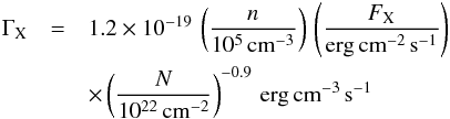 (6)(Maloney
et al. 1996), where n is gas
density in units of cm-3, FX is X-ray flux
density in units of ergcm-2s-1, and N the column
density of hydrogen attenuating the X-ray flux. For the dense cores studied here,
N is of the order of 1023cm-2. In the region
associated with the Galactic center and encompassing a diameter of about 20 arcminutes,
the total X-ray luminosity in the range 2 to 40 KeV (Muno et al. 2004; Koyama et al. 2007;
Yuasa et al. 2008; Dogiel et al. 2010) is 6 × 1036 ergs-1,
yielding an X-ray flux density of 2.0 × 10⁻³
ergcm-2s-1.
(6)(Maloney
et al. 1996), where n is gas
density in units of cm-3, FX is X-ray flux
density in units of ergcm-2s-1, and N the column
density of hydrogen attenuating the X-ray flux. For the dense cores studied here,
N is of the order of 1023cm-2. In the region
associated with the Galactic center and encompassing a diameter of about 20 arcminutes,
the total X-ray luminosity in the range 2 to 40 KeV (Muno et al. 2004; Koyama et al. 2007;
Yuasa et al. 2008; Dogiel et al. 2010) is 6 × 1036 ergs-1,
yielding an X-ray flux density of 2.0 × 10⁻³
ergcm-2s-1.
The gas cooling via gas-dust interaction can be expressed as
 (7)(Tielens
2005), where Tkin
is the gas kinetic temperature and Td dust temperature. For
a gas density range of 104 to 106cm-3, accounting for
the velocity gradient, dv/dr, the
line cooling is approximated well by the expression
(7)(Tielens
2005), where Tkin
is the gas kinetic temperature and Td dust temperature. For
a gas density range of 104 to 106cm-3, accounting for
the velocity gradient, dv/dr, the
line cooling is approximated well by the expression
 (8)(Goldsmith
& Langer 1978; Goldsmith 2001;
Papadopoulos 2010), where
dv/dr is the velocity gradient
adopted to calculate the line cooling rate in the LVG radiative transfer models. The
line cooling is through rotational lines of CO, its isotopologues 13CO and
C18O, and other species (Goldsmith 2001). If the water is highly abundant
in the warm clouds of the CMZ, the line cooling from the water emission will be
important, and this will lead to lower gas kinetic temperatures in this section.
However, this will not drastically change our results, because water is unlikely to be
that dominant. Furthermore, water vapor only affects the cooling rate and not the
heating process, so that our evaluation of relative efficiencies of different heating
processes is not seriously affected.
(8)(Goldsmith
& Langer 1978; Goldsmith 2001;
Papadopoulos 2010), where
dv/dr is the velocity gradient
adopted to calculate the line cooling rate in the LVG radiative transfer models. The
line cooling is through rotational lines of CO, its isotopologues 13CO and
C18O, and other species (Goldsmith 2001). If the water is highly abundant
in the warm clouds of the CMZ, the line cooling from the water emission will be
important, and this will lead to lower gas kinetic temperatures in this section.
However, this will not drastically change our results, because water is unlikely to be
that dominant. Furthermore, water vapor only affects the cooling rate and not the
heating process, so that our evaluation of relative efficiencies of different heating
processes is not seriously affected.
If X-ray heating dominates the heating process, the gas kinetic temperature can be
estimated from the thermal equilibrium
 (9)To simply solve
the equation above, we set the dust temperature to Td = 0K,
yielding a minimum Tkin value and its simple analytic
solution as below
(9)To simply solve
the equation above, we set the dust temperature to Td = 0K,
yielding a minimum Tkin value and its simple analytic
solution as below 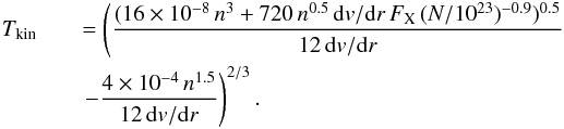 (10)Choosing
a velocity gradient of 5 km s-1pc-1, and adopting the observed
X-ray flux density of 2.0 × 10⁻³ ergcm-2s-1, the
derived gas kinetic temperature is only 1K. It indicates that the observed X-ray flux
density cannot explain the high gas temperatures observed by formaldehyde. Peculiar
conditions in the CMZ, like a potentially high water vapor abundance, enhancing cooling,
or a high magnetic field inhibiting the dissipation of turbulent motion, would not help
to diminish the resulting discrepancy.
(10)Choosing
a velocity gradient of 5 km s-1pc-1, and adopting the observed
X-ray flux density of 2.0 × 10⁻³ ergcm-2s-1, the
derived gas kinetic temperature is only 1K. It indicates that the observed X-ray flux
density cannot explain the high gas temperatures observed by formaldehyde. Peculiar
conditions in the CMZ, like a potentially high water vapor abundance, enhancing cooling,
or a high magnetic field inhibiting the dissipation of turbulent motion, would not help
to diminish the resulting discrepancy.
To simplify this: if the X-ray flux density were about 500 times higher than the
observed value and line cooling dominates the cooling process, we could derive an
approximate gas temperature with
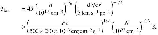 (11)This
equation shows that Tkin depends weakly on the gas density,
velocity gradient, column density of hydrogen attenuating the X-ray emission, and X-ray
flux density. The first three parameters cannot change significantly. If X-rays really
play an important role in heating the gas, an X-ray flux density, about three orders of
magnitude higher than observed, is required. Such an intense X-ray radiation field may
exist in some spatially confined regions. However, it cannot explain the high gas
temperatures on the large spatial scales of the GC. Recent observations (e.g., Eckart et
al. 2012; Nowak et al. 2012) confirm that the X-ray emission from Sgr A∗ shows
flares, almost daily, by factors of a few to ten times over the quiescent emission
level, and rarely even up to more than 100 times that level on time scales from a few
minutes to a few hours. However, this is still much less than what is required to
explain our observed kinetic gas temperatures.
(11)This
equation shows that Tkin depends weakly on the gas density,
velocity gradient, column density of hydrogen attenuating the X-ray emission, and X-ray
flux density. The first three parameters cannot change significantly. If X-rays really
play an important role in heating the gas, an X-ray flux density, about three orders of
magnitude higher than observed, is required. Such an intense X-ray radiation field may
exist in some spatially confined regions. However, it cannot explain the high gas
temperatures on the large spatial scales of the GC. Recent observations (e.g., Eckart et
al. 2012; Nowak et al. 2012) confirm that the X-ray emission from Sgr A∗ shows
flares, almost daily, by factors of a few to ten times over the quiescent emission
level, and rarely even up to more than 100 times that level on time scales from a few
minutes to a few hours. However, this is still much less than what is required to
explain our observed kinetic gas temperatures.
4.4.2. Cosmic-ray heating
For the UV-shielded and mostly subsonic dense gas cores (e.g., dark clouds), cosmic-ray
heating is the major heating process, and it may also play an important role in heating
the gas in the GC because the cosmic-ray flux density is enhanced by the supernovae in
this region. The cosmic-ray heating rate is given by
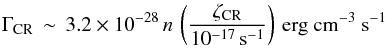 (12)(Goldsmith
& Langer 1978), where
ζCR is the total cosmic-ray ionization rate. If the gas
heating in the GC is dominated by the cosmic-ray heating, we can obtain the gas kinetic
temperature from the energy balance equation
(12)(Goldsmith
& Langer 1978), where
ζCR is the total cosmic-ray ionization rate. If the gas
heating in the GC is dominated by the cosmic-ray heating, we can obtain the gas kinetic
temperature from the energy balance equation
 (13)As above in
Sect. 4.4.1, we set the dust temperature to
Td = 0K, yielding a minimum
Tkin value and the following analytic solution as below
(13)As above in
Sect. 4.4.1, we set the dust temperature to
Td = 0K, yielding a minimum
Tkin value and the following analytic solution as below
 (14)Similarly,
we can obtain a simple solution as below if line cooling dominates the cooling process
(14)Similarly,
we can obtain a simple solution as below if line cooling dominates the cooling process
 (15)If
cosmic-rays are the only heating source, gas temperatures are constrained by three
parameters: gas density, velocity gradient, and the cosmic-ray ionization rate. It is
reasonable to adopt a gas density of 104.5 cm-3 (still low enough
to yield (almost) optically thin H2CO 303 → 202
emission) and a velocity gradient of 5km s-1 pc-1for the clouds in
the GC. The poorly determined parameter is the comic-ray ionization rate. Using the
assumed parameters, the gas kinetic temperatures from Eq. (14) are 22, 54, 70, and 122K
for cosmic-ray ionization rates of 10-15, 10-14, 2 ×
10-14, and 10-13s-1. Thus, if cosmic rays play an
important role in heating the gas, a cosmic-ray ionization rate of at least 1−2 ×
10-14s-1 is required to explain the observed temperatures in the
GC, which is about three orders of magnitude higher than in the solar neighborhood
(e.g., Farquhar et al. 1994). Such an enhanced
flux of cosmic-ray electrons is inferred in SgrB2 by Yusef-Zadeh et al. (2007), and is interpreted as the main molecular-gas
heating source in this region. The required high cosmic ray flux of 1−2 ×
10-14s-1 would lead to an Hi density of about 500
cm-3 (Güsten et al. 1981). Such a
large Hi abundance will cause noticeable 21 cm signals, which have indeed been
seen in Hi absorption surveys toward some GC clouds (e.g., Schwarz et al. 1977; Lang et al. 2010). For comparison, Bradford et al. (2003) estimate that a high supernova rate in the nucleus of NGC253 results in
a cosmic-ray ionization rate of 1.5−5.3 × 10⁻¹⁴s-1. This mechanism
may also play an important role in regulating the gas in ultraluminous infrared galaxies
(ULIRGs) where the cosmic ray energy density may be as high as 1000 times that of the
local Galactic value or even higher (Papadopoulos 2010; Papadopoulos et al. 2011).
(15)If
cosmic-rays are the only heating source, gas temperatures are constrained by three
parameters: gas density, velocity gradient, and the cosmic-ray ionization rate. It is
reasonable to adopt a gas density of 104.5 cm-3 (still low enough
to yield (almost) optically thin H2CO 303 → 202
emission) and a velocity gradient of 5km s-1 pc-1for the clouds in
the GC. The poorly determined parameter is the comic-ray ionization rate. Using the
assumed parameters, the gas kinetic temperatures from Eq. (14) are 22, 54, 70, and 122K
for cosmic-ray ionization rates of 10-15, 10-14, 2 ×
10-14, and 10-13s-1. Thus, if cosmic rays play an
important role in heating the gas, a cosmic-ray ionization rate of at least 1−2 ×
10-14s-1 is required to explain the observed temperatures in the
GC, which is about three orders of magnitude higher than in the solar neighborhood
(e.g., Farquhar et al. 1994). Such an enhanced
flux of cosmic-ray electrons is inferred in SgrB2 by Yusef-Zadeh et al. (2007), and is interpreted as the main molecular-gas
heating source in this region. The required high cosmic ray flux of 1−2 ×
10-14s-1 would lead to an Hi density of about 500
cm-3 (Güsten et al. 1981). Such a
large Hi abundance will cause noticeable 21 cm signals, which have indeed been
seen in Hi absorption surveys toward some GC clouds (e.g., Schwarz et al. 1977; Lang et al. 2010). For comparison, Bradford et al. (2003) estimate that a high supernova rate in the nucleus of NGC253 results in
a cosmic-ray ionization rate of 1.5−5.3 × 10⁻¹⁴s-1. This mechanism
may also play an important role in regulating the gas in ultraluminous infrared galaxies
(ULIRGs) where the cosmic ray energy density may be as high as 1000 times that of the
local Galactic value or even higher (Papadopoulos 2010; Papadopoulos et al. 2011).
4.4.3. Turbulent heating
The dissipation of turbulent kinetic energy provides a potentially important heating
source in Galactic astrophysical environments, such as interstellar clouds (e.g.,
Falgarone & Puget 1995) and the warm
ionized medium (e.g., Minter & Balser 1997), and in extragalactic environments, such as intracluster cooling flows
(Dennis & Chandran 2005). The observed
large velocity dispersion in the GC requires energy input to support the turbulence
because the dynamic timescale is rather short, around 106 years. This implies
a high turbulent heating rate. Following Pan & Padoan (2009), the turbulent heating rate is given by
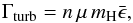 (16)where
n and mH are the number density and the
mass of the hydrogen atom, μ is the mean molecular weight,
μ = 2.35 for molecular clouds, and
(16)where
n and mH are the number density and the
mass of the hydrogen atom, μ is the mean molecular weight,
μ = 2.35 for molecular clouds, and
 is the average dissipation rate per unit mass. The average dissipation rate per unit
mass, is given by
is the average dissipation rate per unit mass. The average dissipation rate per unit
mass, is given by 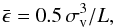 (17)where
σv is the one-dimensional velocity dispersion and
L the size of the cloud. Replacing the expression for
in Eq. (16) and substituting units, the average turbulent heating rate is
(17)where
σv is the one-dimensional velocity dispersion and
L the size of the cloud. Replacing the expression for
in Eq. (16) and substituting units, the average turbulent heating rate is
 (18)where the gas density
n is in units of cm-3, the one-dimensional velocity
dispersion σv is in units of km s-1, and the
cloud size L is in units of pc. We can relate the one-dimensional
velocity dispersion and the observed FWHM line widths by the conversion
σv = VFWHM/2.355 (Pan
& Padoan 2009).
(18)where the gas density
n is in units of cm-3, the one-dimensional velocity
dispersion σv is in units of km s-1, and the
cloud size L is in units of pc. We can relate the one-dimensional
velocity dispersion and the observed FWHM line widths by the conversion
σv = VFWHM/2.355 (Pan
& Padoan 2009).
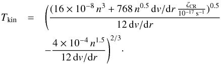
If turbulent heating dominates the heating process, the gas kinetic temperature can be
estimated from thermal equilibrium
 (19)To solve the
equation above simply, we set the dust temperature to
Td = 0K, yielding a minimum Tkin
value and its simple analytic solution as
(19)To solve the
equation above simply, we set the dust temperature to
Td = 0K, yielding a minimum Tkin
value and its simple analytic solution as  (20)Choosing
a velocity gradient of 5 km s-1pc-1, an observed FWHM line width
of 20 km s-1, and a cloud size of 5pc, the derived gas kinetic temperature
ranges between 51 and 62K for a range in gas density of 104 to
105cm-3.
(20)Choosing
a velocity gradient of 5 km s-1pc-1, an observed FWHM line width
of 20 km s-1, and a cloud size of 5pc, the derived gas kinetic temperature
ranges between 51 and 62K for a range in gas density of 104 to
105cm-3.
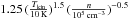
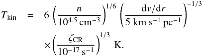
For gas densities n≤105cm-3 and the assumed
parameters as above, line cooling dominates the cooling process and the solution can be
simplified to  (21)This
equation underestimates the gas temperature by less than 10% in comparison with Eq.
(20), and shows that the temperature depends only weakly on the gas density, cloud size,
and velocity gradient, but strongly depends on line width. Considering the line widths
in different clouds, we can use Eq. (20) to calculate the temperatures and present the
results in the last column of Table 1. To compare
the calculated temperatures by turbulent heating with the ones derived from the
H2CO measurements in Sect. 4.3, we
plot both temperatures in Fig. 7. In general, the
temperatures agree within the uncertainties, supporting turbulent heating as a good
candidate to heat the gas to the high temperatures observed in the GC. High gas kinetic
temperatures were also deduced from NH3 absorption lines toward Sgr B2 by
Wilson et al. (1982). They suggested that the
high gas temperatures were caused by turbulence maintained by shearing forces as a
consequence of galactic rotation.
(21)This
equation underestimates the gas temperature by less than 10% in comparison with Eq.
(20), and shows that the temperature depends only weakly on the gas density, cloud size,
and velocity gradient, but strongly depends on line width. Considering the line widths
in different clouds, we can use Eq. (20) to calculate the temperatures and present the
results in the last column of Table 1. To compare
the calculated temperatures by turbulent heating with the ones derived from the
H2CO measurements in Sect. 4.3, we
plot both temperatures in Fig. 7. In general, the
temperatures agree within the uncertainties, supporting turbulent heating as a good
candidate to heat the gas to the high temperatures observed in the GC. High gas kinetic
temperatures were also deduced from NH3 absorption lines toward Sgr B2 by
Wilson et al. (1982). They suggested that the
high gas temperatures were caused by turbulence maintained by shearing forces as a
consequence of galactic rotation.
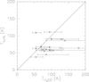 |
Fig. 7 Gas temperatures estimated by turbulent heating versus those derived from the H2CO LVG models with [para-H2CO] = 10-10. The solid line shows the relationship for the cases where both temperatures are the same. |
For turbulent and cosmic-ray heating, we cannot distinguish which mechanism dominates
the heating of molecular clouds in the GC. With a large interferometer such as ALMA, one
can try to search for molecular clumps with thermal line widths, i.e. with line widths
that are dominated by thermal motion. If such objects can be found, turbulent heating
can be excluded because the narrow line widths cannot be explained by turbulent heating,
and the cosmic-ray heating will then be the dominant process to heat the gas to high
temperatures. Future observations of  (the average ionization fraction) can also help distinguish between these two heating
mechanisms, because high cosmic-ray energy densities will boost this fraction, unlike
turbulence (Papadopoulos 2010 and references
therein).
(the average ionization fraction) can also help distinguish between these two heating
mechanisms, because high cosmic-ray energy densities will boost this fraction, unlike
turbulence (Papadopoulos 2010 and references
therein).
The special thermal state of the GC clouds may be the average state of the molecular ISM in ULIRGs, with a direct impact on their stellar IMF (Papadopoulos et al. 2011). The high temperatures of molecular clouds on large scales in the GC region may be driven by turbulent energy dissipation and/or cosmic-rays instead of photons. Such a non-photon-driven thermal state of the molecular gas provides an excellent template for studying the intial conditions and star formation for the galaxy-sized gas in ULIRGs.
5. Conclusions
The JKAKc = 303 → 202, 322 → 221, and 321 → 220 transitions of para-H2CO were observed simultaneously with the APEX telescope, covering an area of roughly 40′ × 8′ along the Galactic plane with a linear resolution of 1.2pc, including the Galactic center. The main results from these measurements follow.
-
(1)
The strongest line of the 218GHz H2CO triplet, H2CO (303 → 202), is widespread in the mapped region, and its emission shows a morphology similar to ammonia (Güsten et al. 1981).
-
(2)
The para-H2CO abundance is found to be 0.5−1.2 × 10⁻⁹, which is consistent with previous studies of formaldehyde absorption lines at cm-wavelengths in the Galactic center region.
-
(3)
Using LVG models, we can constrain gas kinetic temperatures to be of about 85 K for the Galactic center clouds, ranging from 50 to values above 100 K. While a systematic trend of (decreasing) kinetic temperature versus (increasing) angular distance from the nucleus is not found, the clouds with highest temperature (Tkin> 100K) are all located near the center. Molecular gas outside of the dense cores in the Galactic center region is characterized by a gas kinetic temperature of 65 ± 10 K.
-
(4)
The high temperatures found in the Galactic center region may be caused by turbulent heating and/or cosmic-ray heating. Turbulent heating can readily heat the gas to the values deduced from H2CO. If cosmic-ray heating dominates the heating process, a cosmic-ray ionization rate of at least 1−2 × 10-14 is required to explain the observed temperatures. The high temperatures of molecular clouds on large scales in the Galactic center region may be driven by turbulent energy dissipation and/or cosmic-rays instead of photons. Such a non-photon-driven thermal state of the molecular gas make such clouds excellent templates for the starbursts found in ultraluminous infrared galaxies.
Online material
Appendix A: H2CO line parameters
Line parameters.
Appendix B:
B.1. H2CO spectral lines
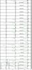 |
Fig. B.1 Spectra of different positions marked by the numbers in Fig. 2. All transitions from a given position are presented in the
same panel but with different offsets along the y-axis on a
|
B.2. Velocity channel maps
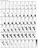 |
Fig. B.2 Channel maps of the H2CO 303 − 202 emission.
Black contour levels for the molecular line emission (on a
|
NH3 energy levels have quantum numbers (J,K), where J denotes the total angular momentum and K its projection on the molecule’s axis. For metastable levels, J=K.
This publication is based on data acquired with the Atacama Pathnder Experiment (APEX). APEX is a collaboration between the Max-Planck-Institut für Radioastronomie, the European Southern Observatory, and the Onsala Space Observatory.
Acknowledgments
We thank the anonymous referee and the Editor Malcolm Walmsley for valuable comments that improved this manuscript. We wish to thank Padelis Papadopoulos for useful discussions. Y.A. acknowledges the supports by the grant 11003044 from the National Natural Science Foundation of China, and 2009’s President Excellent Thesis Award of the Chinese Academy of Sciences. This research has made use of NASAs Astrophysical Data System (ADS).
References
- Alexander, R. D., Begelman, M. C., & Armitage, P. J. 2007, ApJ, 654, 907 [NASA ADS] [CrossRef] [Google Scholar]
- Amo-Baladrón, M. A., Martín-Pintado, J., Morris, M. R., Muno, M. P., & Rodríguez-Fernández, N. J. 2009, ApJ, 694, 943 [NASA ADS] [CrossRef] [Google Scholar]
- Arons, J., & Max, C. E. 1975, ApJ, 196, L77 [NASA ADS] [CrossRef] [Google Scholar]
- Bally, J., Stark, A. A., Wilson, R. W., & Henkel, C. 1987, ApJS, 65, 13 [NASA ADS] [CrossRef] [Google Scholar]
- Bartko, H., Martins, F., Trippe, S., et al. 2010, ApJ, 708, 834 [NASA ADS] [CrossRef] [Google Scholar]
- Bradford, C. M., Nikola, T., Stacey, G. J., et al. 2003, ApJ, 586, 891 [NASA ADS] [CrossRef] [Google Scholar]
- Caselli, P., Hasegawa, T. I., & Herbst, E. 1993, ApJ, 408, 548 [NASA ADS] [CrossRef] [Google Scholar]
- Croker, P. M., Jones, D. L., Melia, F., Ott, J., & Protheroe, R. J. 2010, Nature, 463, 65 [NASA ADS] [CrossRef] [Google Scholar]
- Dahmen, G., Hüttemeister, S., Wilson, T. L., & Mauersberger, R. 1998, A&A, 331, 959 [NASA ADS] [Google Scholar]
- Dame, T. M. 2011, [arXiv:1101.1499] [Google Scholar]
- Dame, T. M., Ungerechts, H., Cohen, R. S., et al. 1987, ApJ, 322, 706 [NASA ADS] [CrossRef] [Google Scholar]
- Dame, T. M., Hartmann, D., & Thaddeus, P. 2001, ApJ, 547, 792 [NASA ADS] [CrossRef] [Google Scholar]
- Danby, G., Flower, D. R., Valiron, P., Schilke, P., & Walmsley, C. M. 1988, MNRAS, 235, 229 [NASA ADS] [CrossRef] [Google Scholar]
- Dennis, T. J., & Chandran, B. D. G. 2005, ApJ, 622, 205 [NASA ADS] [CrossRef] [Google Scholar]
- Dogiel, V. A., Cheng, K.-S., Chernyshov, D. O., et al. 2011, in The Galactic Center: a Window to the Nuclear Environment of Disk Galaxies, eds. M. R. Morris, Q. D. Wang, & F. Yuan (San Francisco: ASP), 426 [Google Scholar]
- Eckart, A., García-Marín, M., Vogel, S. N., et al. 2012, A&A, 537, A52 [NASA ADS] [CrossRef] [EDP Sciences] [Google Scholar]
- Falgarone, E., & Puget, J.-L. 1995, A&A, 293, 840 [NASA ADS] [Google Scholar]
- Farquhar, P. R. A., Millar, T. J., & Herbst, E. 1994, MNRAS, 269, 641 [NASA ADS] [CrossRef] [Google Scholar]
- Ferriére, K. 2009, A&A, 505, 1183 [NASA ADS] [CrossRef] [EDP Sciences] [Google Scholar]
- García-Marín, M., Eckart, A., Weiss, A., et al. 2011, ApJ, 738, 158 [NASA ADS] [CrossRef] [Google Scholar]
- Goldsmith, P. F., & Langer, W. D. 1978, ApJ, 222, 881 [NASA ADS] [CrossRef] [Google Scholar]
- Green, S. 1991, ApJS, 76, 979 [NASA ADS] [CrossRef] [Google Scholar]
- Güsten, R., & Henkel, C. 1983, A&A, 125, 136 [NASA ADS] [Google Scholar]
- Güsten, R., & Philipp, S. D. 2004, The Dense Interstellar Medium in Galaxies, 253 [Google Scholar]
- Güsten, R., Walmsley, C. M., & Pauls, T. 1981, A&A, 103, 197 [NASA ADS] [Google Scholar]
- Güsten, R., Henkel, C., & Batrla, W. 1985a, A&A, 149, 195 [NASA ADS] [Google Scholar]
- Güsten, R., Walmsley, C. M., Ungerechts, H., & Churchwell, E. 1985b, A&A, 142, 381 [NASA ADS] [Google Scholar]
- Güsten, R., Nyman, L. Å., Schilke, P., et al. 2006, A&A, 454, L13 [NASA ADS] [CrossRef] [EDP Sciences] [Google Scholar]
- Hollenbach, D. J., & Tielens, A. G. G. M. 1999, Rev. Mod. Phys., 71, 173 [Google Scholar]
- Hüttemeister, S., Dahmen, G., Mauersberger, R., et al. 1998, A&A, 334, 646 [NASA ADS] [Google Scholar]
- Hüttemeister, S., Wilson, T. L., Bania, T. M., & Martin-Pintado, J. 1993, A&A, 280, 255 [NASA ADS] [Google Scholar]
- Johnstone, D., Boonman, A. M. S., & van Dishoeck, E. F. 2003, A&A, 412, 157 [NASA ADS] [CrossRef] [EDP Sciences] [Google Scholar]
- Jones, P. A., Burton, M. G., Cunningham, M. R., et al. 2012, MNRAS, 419, 2961 [NASA ADS] [CrossRef] [Google Scholar]
- Kim, S., Martin, C. L., Stark, A. A., & Lane, A. P. 2002, ApJ, 580, 896 [NASA ADS] [CrossRef] [Google Scholar]
- Klein, B., Philipp, S. D., Krämer, I., et al. 2006, A&A, 454, L29 [NASA ADS] [CrossRef] [EDP Sciences] [Google Scholar]
- Klessen, R. S., Spaans, M., & Jappsen, A.-K. 2007, MNRAS, 374, L29 [NASA ADS] [CrossRef] [Google Scholar]
- Koyama, K., Hyodo, Y., Inui, T., et al. 2007, PASJ, 59, 245 [NASA ADS] [Google Scholar]
- Krügel, E., & Walmsley, C. M. 1984, A&A, 130, 5 [NASA ADS] [Google Scholar]
- Lang, C. C., Goss, W. M., Cyganowski, C., & Clubb, K. I. 2010, ApJS, 191, 275 [NASA ADS] [CrossRef] [Google Scholar]
- Mühle, S., Seaquist, E. R., & Henkel, C. 2007, ApJ, 671, 1579 [NASA ADS] [CrossRef] [Google Scholar]
- Maloney, P. R., Hollenbach, D. J., & Tielens, A. G. G. M. 1996, ApJ, 466, 561 [NASA ADS] [CrossRef] [Google Scholar]
- Mangum, J. G., & Wootten, A. 1993a, ApJS, 89, 123 [NASA ADS] [CrossRef] [Google Scholar]
- Mangum, J. G., Wootten, A., & Plambeck, R. L. 1993b, ApJ, 409, 282 [NASA ADS] [CrossRef] [Google Scholar]
- Martin-Pintado, J., de Vicente, P., Fuente, A., & Planesas, P. 1997, ApJ, 482, L45 [NASA ADS] [CrossRef] [Google Scholar]
- Mauersberger, R., Henkel, C., Weiß, A., Peck, A. B., & Hagiwara, Y. 2003, A&A, 403, 561 [NASA ADS] [CrossRef] [EDP Sciences] [Google Scholar]
- Mauersberger, R., Henkel, C., Wilson, T. L., & Walmsley, C. M. 1986, A&A, 162, 199 [NASA ADS] [Google Scholar]
- Mauersberger, R., Henkel, C., & Wilson, T. L. 1987, A&A, 173, 352 [NASA ADS] [Google Scholar]
- Minter, A. H., & Balser, D. S. 1997, ApJ, 484, L133 [NASA ADS] [CrossRef] [Google Scholar]
- Molinari, S., Bally, J., Noriega-Crespo, A., et al. 2011, ApJ, 735, L33 [NASA ADS] [CrossRef] [Google Scholar]
- Morris, M., & Serabyn, E. 1996, ARA&A, 34, 645 [NASA ADS] [CrossRef] [Google Scholar]
- Mundy, L. G., Evans, N. J., II, Snell, R. L., & Goldsmith, P. F. 1987, ApJ, 318, 392 [NASA ADS] [CrossRef] [Google Scholar]
- Muno, M. P., Baganoff, F. K., Bautz, M. W., et al. 2004, ApJ, 613, 326 [NASA ADS] [CrossRef] [Google Scholar]
- Myers, P. C., & Benson, P. J. 1983, ApJ, 266, 309 [NASA ADS] [CrossRef] [Google Scholar]
- Nagai, M., Tanaka, K., Kamegai, K., & Oka, T. 2007, PASJ, 59, 25 [NASA ADS] [Google Scholar]
- Nowak, M. A., Neilsen, J., Markoff, S. B., et al. 2012, ApJ, 759, 95 [NASA ADS] [CrossRef] [Google Scholar]
- Nummelin, A., Bergman, P., Hjalmarson, Å., et al. 2000, ApJS, 128, 213 [NASA ADS] [CrossRef] [Google Scholar]
- Nummelin, A., Bergman, P., Hjalmarson, A., et al. 1998, ApJS, 117, 427 [NASA ADS] [CrossRef] [Google Scholar]
- Oka, T., Nagai, M., Kamegai, K., & Tanaka, K. 2011, ApJ, 732, 120 [NASA ADS] [CrossRef] [Google Scholar]
- Pan, L., & Padoan, P. 2009, ApJ, 692, 594 [NASA ADS] [CrossRef] [Google Scholar]
- Papadopoulos, P. P. 2010, ApJ, 720, 226 [NASA ADS] [CrossRef] [Google Scholar]
- Papadopoulos, P. P., Thi, W.-F., Miniati, F., & Viti, S. 2011, MNRAS, 414, 1705 [NASA ADS] [CrossRef] [Google Scholar]
- Pierce-Price, D., Richer, J. S., Greaves, J. S., et al. 2000, ApJ, 545, L121 [Google Scholar]
- Reid, M. J. 1993, ARA&A, 31, 345 [NASA ADS] [CrossRef] [Google Scholar]
- Requena-Torres, M. A., Martín-Pintado, J., Rodríguez-Franco, A., et al. 2006, A&A, 455, 971 [NASA ADS] [CrossRef] [EDP Sciences] [Google Scholar]
- Rodríguez-Fernández, N. J., Martín-Pintado, J., Fuente, A., & Wilson, T. L. 2004, A&A, 427, 217 [NASA ADS] [CrossRef] [EDP Sciences] [Google Scholar]
- Scalo, J. M. 1977, ApJ, 213, 705 [NASA ADS] [CrossRef] [Google Scholar]
- Schulz, A., Güsten, R., Köster, B., & Krause, D. 2001, A&A, 371, 25 [NASA ADS] [CrossRef] [EDP Sciences] [Google Scholar]
- Schwarz, U. J., Shaver, P. A., & Ekers, R. D. 1977, A&A, 54, 863 [NASA ADS] [Google Scholar]
- Tielens, A. G. G. M. (ed.) 2005, The Physics and Chemistry of the Interstellar Medium (Cambridge: Cambridge Univ. Press) [Google Scholar]
- Walmsley, C. M., & Ungerechts, H. 1983, A&A, 122, 164 [NASA ADS] [Google Scholar]
- Weiß, A., Neininger, N., Henkel, C., Stutzki, J., & Klein, U. 2001, ApJ, 554, L143 [NASA ADS] [CrossRef] [Google Scholar]
- Wilson, T. L., Ruf, K., Walmsley, C. M., et al. 1982, A&A, 115, 185 [NASA ADS] [Google Scholar]
- Wootten, A., Evans, N. J., II Snell, R., & van den Bout, P. 1978, ApJ, 225, L143 [NASA ADS] [CrossRef] [Google Scholar]
- Yuasa, T., Tamura, K.-I., Nakazawa, K., et al. 2008, PASJ, 60, 207 [Google Scholar]
- Yusef-Zadeh, F., Wardle, M., & Roy, S. 2007, ApJ, 665, L123 [NASA ADS] [CrossRef] [Google Scholar]
- Zylka, R., Güsten, R., Henkel, C., & Batrla, W. 1992, A&AS, 96, 525 [NASA ADS] [Google Scholar]
All Tables
All Figures
|
Fig. 1 H2CO energy-level diagram up to 200K. The H2CO 218GHz transitions observed in this paper are shown in bold. |
| In the text | |
|
Fig. 2 H2CO (303 → 202) integrated intensity map (left)
and the noise map (right) observed with the APEX in the GC. Left:
black contour levels for the molecular line emission (on a
|
| In the text | |
|
Fig. 3 Integrated intensity maps for the different transitions observed in the GC. The shown
region corresponds to the rectangle (black solid line) in Fig. 2 (left). Black contour levels for the molecular
line emission (on a |
| In the text | |
|
Fig. 4 Selected velocity-integrated maps for the different transitions observed in the GC.
Black contour levels for the molecular line emission (on a
|
| In the text | |
|
Fig. 5 H2CO 322 → 221/303 → 202 (top) and 321 → 220/303 → 202 (bottom) integrated intensity ratio map. Ratios are calculated when the H2CO 303 → 202 line emission is detected above 5σ. The top and bottom rows should be nearly identical, and the difference mainly comes from the CH3OH contamination in H2CO 322 → 221. The wedges at the sides show the line ratios. The beam size of 30″ is shown at the bottom-left corner. Sgr A∗ is the origin for the offset coordinates and shown as a cross. |
| In the text | |
|
Fig. 6 Example of LVG modeling for P4. Top: reduced χ2 distribution (mainly vertical contours) for a single-component LVG model fit to the H2CO brightness temperatures (black contours, χ2=1,2,4), as well as H2CO 322 → 221/303 → 202 line ratios (mainly horizonal contours) as a function of nH2 and Tkin. The solid lines represent the line ratios: 0.05, 0.1, 0.15, 0.2, 0.25, 0.3, 0.35, 0.4. The red dashed lines show the observed line ratio and its lower and upper limits. The para-H2CO abundances per velocity gradient, [para-H2CO]/(dv/dr), for the LVG models are 2 × 10⁻¹⁰ pc(km s-1)-1 (left) and 2 × 10-11pc(km s-1)-1 (right), respectively. In the left panel the lines with a given H2CO line ratio move downwards (lower Tkin) at high density because the H2CO lines start to become saturated; this causes intensity ratios for a given Tkin to get closer to unity. Bottom: reduced χ2 distribution for the H2CO 321 → 220/303 → 202 line ratios. The kinetic temperature is sensitive to the gas density so this line ratio is a less suitable thermometer. |
| In the text | |
|
Fig. 7 Gas temperatures estimated by turbulent heating versus those derived from the H2CO LVG models with [para-H2CO] = 10-10. The solid line shows the relationship for the cases where both temperatures are the same. |
| In the text | |
|
Fig. B.1 Spectra of different positions marked by the numbers in Fig. 2. All transitions from a given position are presented in the
same panel but with different offsets along the y-axis on a
|
| In the text | |
|
Fig. B.2 Channel maps of the H2CO 303 − 202 emission.
Black contour levels for the molecular line emission (on a
|
| In the text | |
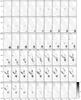 |
Fig. B.3 Same as Fig. B.2 but for the H2CO 322 − 221 emission. |
| In the text | |
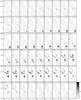 |
Fig. B.4 Same as Fig. B.2 but for the H2CO 321 − 220 emission. |
| In the text | |
Current usage metrics show cumulative count of Article Views (full-text article views including HTML views, PDF and ePub downloads, according to the available data) and Abstracts Views on Vision4Press platform.
Data correspond to usage on the plateform after 2015. The current usage metrics is available 48-96 hours after online publication and is updated daily on week days.
Initial download of the metrics may take a while.