© ESO, 2013

1. Introduction

The magnetic fields configuration is essential for us to understand solar explosive phenomena, such as flares and coronal mass ejections. The corona has been the subject of extensive modeling for decades, but these efforts have been hampered by our limited ability to determine the corona’s three-dimensional structure (Schrijver & Title 2011; Sandman & Aschwanden 2011). Since the corona is optically thin, direct measurements of these magnetic fields are very difficult to implement, and the present observations for the magnetic fields based on the spectropolarimetric method (the Zeeman and the Hanle effects) are limited to low layers of solar atmosphere (photosphere and chromosphere). The problem of measuring the coronal field and its embedded electrical currents thus leads us to use numerical modeling to infer the field strength in the higher layers of the solar atmosphere from the measured photospheric field. Owing the low value of the plasma β (the ratio of gas pressure to magnetic pressure), the solar corona is magnetically dominated (Gary 2001). To describe the equilibrium structure of the static coronal magnetic field when nonmagnetic forces are negligible, the force-free assumption is appropriate: $\begin{array}{ccc}& & \mathrm{(}\mathrm{\nabla }\mathrm{\times }{B}\mathrm{)}\mathrm{\times }{B}\mathrm{=}\mathrm{0}\\ & & \mathrm{\nabla }\mathrm{·}{B}\mathrm{=}\mathrm{0}\end{array}$subject to the boundary condition ${B}\mathrm{=}{B}\mathrm{obs} \mathrm{onphotosphere}\mathit{,}$(3)where B is the magnetic field, and B_obs is measured vector field on the photosphere. Equation (1) states that the Lorentz force vanishes (as a consequence of J ∥ B, where J is the electric current density) and Eq. (2) describes the absence of magnetic monopoles. Based on the above assumption, the coronal magnetic field is modeled with a nonlinear force-free field (NLFFF) extrapolation (Inhester & Wiegelmann 2006; Valori et al. 2005; Wiegelmann 2004; Wheatland 2004; Wheatland & Régnier 2009; Tadesse et al. 2009; Wheatland & Leka 2011; Amari & Aly 2010; Wiegelmann et al. 2012; Jiang & Feng 2012). From a mathematical point of view, appropriate boundary condition for force-free modeling are the vertical magnetic field B_n and the vertical current J_n prescribed only for one polarity of B_n (Amari et al. 1997, 1999, 2006). A direct use of these boundary conditions is implemented in Grad-Rubin codes (Amari et al. 1999). Wheatland & Régnier (2009) and Wheatland & Leka (2011) implemented the use of ${\mathit{B}}_{\mathit{n}}^{\mathrm{+}}$ and ${\mathit{B}}_{\mathit{n}}^{\mathrm{-}}$ solution together with an error approximation to derive consistent solutions. Using the three components of B as boundary condition requires consistent magnetograms, as outlined in Aly (1989). We use preprocessing and relaxation of the boundary condition to derive these consistent data on the boundary.

As an alternative to real measurement, NLFFF models are thought to be viable tools for investigating the structure, dynamics, and evolution of the coronae of solar active regions. It has been found that NLFFF models are successful in application to analytic test cases (Schrijver et al. 2006; Metcalf et al. 2008), but they are less successful in application to real solar data. However, NLFFF models have been adopted to study various magnetic field structures and properties in the solar atmosphere. For instance, Régnier et al. (2002); Régnier & Amari (2004); Canou et al. (2009); Canou & Amari (2010); Guo et al. (2010); Valori et al. (2012) have substantially studied various magnetic field structures and properties using their respective NLFFF model codes. Different NLFFF models have been found to have markedly different field line configurations and to provide widely varying estimates of the magnetic free energy in the coronal volume, when applied to solar data (DeRosa et al. 2009). The main reasons for that problem are (1) the forces acting on the field within the photosphere; (2) the uncertainties on vector-field measurements, particularly on the transverse component; and (3) the large domain that needs to be modeled to capture the connections of an active region to its surroundings (Tadesse et al. 2011, 2012a). In this study, we have considered those three points explicitly into account. However, caution must still be needed while assessing results from this modeling. This is because many aspects of the specific approach to modeling used in this work, such as the use of preprocessed boundary data, the missing boundary data, and the departure of the model fields from the observed boundary fields may influence the results.

In this work, we use full-disk SDO/HMI and SOLIS/VSM photospheric magnetic field measurements to model the nonlinear force-free coronal field above multiple solar active regions. Comparison of vector magnetograms for one particular active region observed with two different instruments from SOLIS and HMI and their corresponding force-free models have been studied by Thalmann et al. (2012) in Cartesian coordinates. We use a larger computational domain which accommodates most of the connectivity within the coronal region. We use a spherical version of the optimization procedure that has been implemented in Tadesse et al. (2011). We compare quantities like the total magnetic energy content and free magnetic energy and the longitudinal distribution of the magnetic pressure in the HMI and VSM-based model volumes in spherical geometry. We relate the appearing differences to the photospheric quantities such as the magnetic fluxes and electric currents but also show the extent of agreement of NLFFF extrapolations from different data sources.

2. Instrumentation and data set

2.1. Solar Dynamics Observatory (SDO) – Helioseismic and Magnetic Imager (HMI)

The Helioseismic and Magnetic Imager (HMI; Schou et al. 2012) is part of the Solar Dynamics Observatory (SDO) and observes the full Sun at six wavelengths and full Stokes profile in the Fe I 617.3 nm spectral line. HMI consists of a refracting telescope, a polarization selector, an image stabilization system, a narrow band tunable filter and two 4096 pixel CCD cameras with mechanical shutters and control electronics. Photospheric line-of-sight LOS and vector magnetograms are retrieved from filtergrams with a plate scale of 0.5 arc-second. From filtergrams averaged over about ten minutes, Stokes parameters are derived and inverted using the Milne-Eddington (ME) inversion algorithm of Borrero et al. (2011) (the filling factor is held at unity). Within automatically identified regions of strong magnetic fluxes (Turmon et al. 2010), the full disk inversion data are from the second HMI vector data release (JSOC data series hmi.ME_720s_e15w1332). The 180-degree azimuthal ambiguity in the strong field region is resolved using the minimum energy algorithm (Metcalf 1994; Metcalf et al. 2006; Leka et al. 2009), taken from the AR patches in the second release also (data series hmi.B_720s_e15w1332_cutout). For the weak field region where noise dominates, we adopt a radial-acute angle method to resolve the azimuthal ambiguity. The weak field region is defined as where field strength is below 200 G at disk center, 400 G on the limb, and varies linearly in between. The noise level is  ≈ 10 G and  ≈ 100 G for the longitudinal and transverse magnetic field, respectively.

2.2. Synoptic Optical Long-term Investigations of the Sun (SOLIS) – Vector-SpectroMagnetograph (VSM)

The Vector Spectromagnetograph (VSM; see Jones et al. 2002) is part of the Synoptic Optical Long-term Investigations of the Sun (SOLIS) synoptic facility (SOLIS; see Keller et al. 2003). VSM is a full disk Stokes polarimeter. As part of daily synoptic observations, it takes four different observations in three spectral lines: Stokes I (intensity), V (circular polarization), Q, and U (linear polarization) in photospheric spectral lines Fe I 630.15 nm and Fe I 630.25 nm, Stokes I and V in Fe I 630.15 nm and Fe I 630.25 nm, similar observations in chromospheric spectral line Ca II 854.2 nm, and Stokes I in the He I 1083.0 nm line and the near by Si I spectral line. Observations of I, Q, U, and V are used to construct full disk vector magnetograms, while I − V observations are employed to create separate full disk longitudinal magnetograms in the photosphere and the chromosphere. The vector data are provided with a plate scale of one arc-second. The lower limits for the noise levels are a few Gauss in the longitudinal and 70 G in the transverse field measurements.

Quick-look (QL) vector magnetograms were created based on an algorithm by Auer et al. (1977). Beginning January 2012, QL vector magnetograms are created using weak-field approximation (Ronan et al. 1987). The algorithm uses the Milne-Eddington model of solar atmosphere, which assumes that the magnetic field is uniform (no gradients) through the layer of spectral line formation (Unno 1956). It also assumes symmetric line profiles, disregards magneto-optical effects (e.g., Faraday rotation), and does not distinguish the contributions of magnetic and nonmagnetic components in spectral line profiles (i.e., magnetic filling factor is set to unity). A complete inversion of the spectral data is performed later using a technique developed by Skumanich & Lites (1987). This latter inversion (called ME magnetogram) also employs Milne-Eddington model of atmosphere, but solves for magneto-optical effects and determines the magnetic filling factor. The ME inversion is only performed for pixels with spectral line profiles above the noise level. For pixels below the polarimetric noise threshold, the magnetic field parameters are set to zero.

From the measurements, the azimuths of transverse magnetic field can be determined with 180-degree ambiguity. This ambiguity is resolved using the nonpotential field calculation (NPFC; see Georgoulis 2005). The NPFC method was selected on the basis of a comparative investigation of several methods for 180-degree ambiguity resolution (Metcalf et al. 2006). Both QL and ME magnetograms can be used for potential and/or force-free field extrapolation. However, in strong fields inside sunspots, the QL field strengths may exhibit an erroneous decrease inside the sunspot umbra due to so-called magnetic saturation. For this study, we choose to use fully inverted ME magnetograms.

3. Method

Photospheric field measurements are often subject to measurement errors. In addition to this, there are finite nonmagnetic forces which make the data inconsistent as a boundary for a force-free field in the corona. In order to deal with these uncertainties, one has to: 1.) preprocess the surface measurements in order to make them compatible with a force-free field and 2.) keep a balance between the force-free constraint and deviation from the photospheric field measurements. Both methods contain free parameters, which have to be optimized for use with data from SOLIS/VSM and SDO/HMI.

3.1. Preprocessing of HMI and VSM data

To serve as suitable lower boundary condition for a force-free modeling, vector magnetograms have to be approximately flux balanced and on average a net tangential force acting on the boundary and shear stresses along axes lying on the boundary have to reduce to zero. We use dimensionless parameters, ϵ_flux, ϵ_force and ϵ_torque, to quantify such properties (Wiegelmann et al. 2006; Tadesse et al. 2009; Aly 1989; Molodensky 1969). Even if we choose a sufficiently flux balanced region (ϵ_flux), we find that the force-free conditions ϵ_force ≪ 1 and ϵ_torque ≪ 1 are not usually fulfilled for measured vector magnetograms. In order to fulfill those conditions, we use preprocessing method as implemented in Wiegelmann et al. (2006). The preprocessing scheme of Tadesse et al. (2009) involves minimizing a two-dimensional functional of quadratic form in spherical geometry similar to $\begin{array}{ccc}& & {B}\mathrm{=}\mathrm{argmin}\mathrm{\left(}{\mathit{L}}_{\mathrm{p}}\mathrm{\right)}\mathit{,}\\ & & {\mathit{L}}_{\mathrm{p}}\mathrm{=}{\mathit{\mu }}_{\mathrm{1}}{\mathit{L}}_{\mathrm{1}}\mathrm{+}{\mathit{\mu }}_{\mathrm{2}}{\mathit{L}}_{\mathrm{2}}\mathrm{+}{\mathit{\mu }}_{\mathrm{3}}{\mathit{L}}_{\mathrm{3}}\mathrm{+}{\mathit{\mu }}_{\mathrm{4}}{\mathit{L}}_{\mathrm{4}}\mathit{,}\end{array}$(4)where B is the preprocessed surface magnetic field from the input observed field B_obs. Each of the constraints L_n is weighted by an as yet undetermined factor μ_n. The first term (n = 1) corresponds to the force-balance condition, the next (n = 2) to the torque-free condition, and the last term (n = 4) controls the smoothing. The explicit form of L₁, L₂, and L₄ can be found in Tadesse et al. (2009). The term (n = 3) controls the difference between measured and preprocessed vector fields.

3.2. Optimization principle

We solve the force-free Eqs. (1) and (2) by optimization principle, as proposed by Wheatland et al. (2000) and generalized by Wiegelmann (2004) for cartesian geometry. The method minimizes a joint measure of the normalized Lorentz forces and the divergence of the field throughout the volume of interest, V. Throughout this minimization, the photospheric boundary of the model field B is matched exactly to the observed B_obs and possibly preprocessed magnetogram values B. Here, we use the optimization approach for functional (L_ω) in spherical geometry (Wiegelmann 2007; Tadesse et al. 2009) along with the new method, which instead of an exact match enforces a minimal deviation between the photospheric boundary of the model field B and the magnetogram field B_obs by adding an appropriate surface integral term L_photo (Wiegelmann & Inhester 2010; Tadesse et al. 2011). These terms are given by $\begin{array}{ccc}& & {B}\mathrm{=}\mathrm{argmin}\mathrm{\left(}{\mathit{L}}_{\mathit{\omega }}\mathrm{\right)}\\ & & {\mathit{L}}_{\mathit{\omega }}\mathrm{=}{\mathit{L}}_{\mathrm{f}}\mathrm{+}{\mathit{L}}_{\mathrm{d}}\mathrm{+}\mathit{\nu }{\mathit{L}}_{\mathrm{photo}}\\ & & {\mathit{L}}_{\mathrm{f}}\mathrm{=}{\mathrm{\int }}_{\mathit{V}}{\mathit{\omega }}_{\mathrm{f}}\mathrm{\left(}\mathit{r,\theta ,\phi }\mathrm{\right)}{\mathit{B}}^{-2}|\mathrm{(}\mathrm{\nabla }\mathrm{\times }{B}\mathrm{)}\mathrm{\times }{B}{|}^{\mathrm{2}}{\mathit{r}}^{\mathrm{2}}\sin \mathit{\theta }\mathrm{d}\mathit{r}\mathrm{d}\mathit{\theta }\mathrm{d}\mathit{\phi }\\ & & {\mathit{L}}_{\mathrm{d}}\mathrm{=}{\mathrm{\int }}_{\mathit{V}}{\mathit{\omega }}_{\mathrm{d}}\mathrm{\left(}\mathit{r,\theta ,\phi }\mathrm{\right)}|\mathrm{\nabla }\mathrm{·}{B}{|}^{\mathrm{2}}{\mathit{r}}^{\mathrm{2}}\sin \mathit{\theta }\mathrm{d}\mathit{r}\mathrm{d}\mathit{\theta }\mathrm{d}\mathit{\phi }\\ & & {\mathit{L}}_{\mathrm{photo}}\mathrm{=}{\mathrm{\int }}_{\mathit{S}}({B}\mathrm{-}{B}\mathrm{obs})\mathrm{·}{W}\mathrm{\left(}\mathit{\theta ,\phi }\mathrm{\right)}\mathrm{·}({B}\mathrm{-}{B}\mathrm{obs}){\mathit{r}}^{\mathrm{2}}\sin \mathit{\theta }\mathrm{d}\mathit{\theta }\mathrm{d}\mathit{\phi }\end{array}$(5)where L_f and L_d measure how well the force-free Eqs. (1) and divergence-free (2) conditions are fulfilled, respectively, and both ω_f(r, θ, φ) and ω_d(r, θ, φ) are weighting functions. The weighting functions ω_f and ω_d in L_f and L_d in Eq. (5) are chosen to be unity within the inner physical domain V′ and decline with a cosine profile in the buffer boundary region (Wiegelmann 2004; Tadesse et al. 2009, 2012b). They reach a zero value at the boundary of the outer volume V. The distance between the boundaries of V′ and V is chosen to be nd = 10 grid points wide. The third integral, L_photo, is the surface integral over the photosphere which allows us to relax the field on the photosphere towards force-free solution without too much deviation from the original surface field data.

W(θ, φ) is a space-dependent diagonal matrix the element of which are inverse proportional to the estimated squared measurement error of the respective field component. In principle one could compute W from the measurement noise and errors obtained from the inversion of measured Stokes profiles to field components. Until these quantities become available, a reasonable assumption is that the magnetic field is measured in strong field regions more accurately than in the weak field and that the error in the photospheric transverse field is at least one order of magnitude higher as the line-of-sight component. Appropriate choices to optimize ν and W for use with SDO/HMI (Wiegelmann et al. 2012) and SOLIS/VSM (Tadesse et al. 2011) magnetograms have been investigated. For a detailed description of the current code implementation, we refer to Wiegelmann & Inhester (2010) and Tadesse et al. (2011).

4. Results

Within this work, we use the full disk data from SOLIS/VSM and SDO/HMI instruments obsrved on November 09, 2011 around 17:45UT. During this observation there were four active regions (ARs 11338, 11339, 11341 and 11342) along with other smaller sunspots spreading on the disk. To accommodate the connectivity between those ARs and their surroundings, we adopt a non uniform spherical grid r, θ, φ with n_r = 225, n_θ = 375, n_φ = 425 grid points in the direction of radius, latitude, and longitude, respectively, with the field of view of  [r_min = 1   R_⊙:   r_max = 2   R_⊙]  ×  [θ_min = −50°:   θ_max = 50°]  ×  [φ_min = 90°:   φ_max = 270°] . Given the twice as large plate scale of VSM, we bin the HMI vector maps to the resolution of VSM in order to compare the photospheric magnetic field and subsequent force free modeling. To deal with vector magnetogram data being inconsistent with the force-free assumption, we use a preprocessing routine in spherical geometry, which derives suitable boundary conditions for force-free modeling from the measured photospheric data. Applying this procedure to both SDO/HMI and SOLIS/VSM reduces ϵ_force and ϵ_torque further significantly. The two quantities are very well below unity after preprocessing, which gives us some confidence that the data might serve as suitable boundary condition for a force-free modeling. Doing this, we do not intend to suppress the existing forces in the photosphere. Instead, we try to approximate the magnetic field at a chromospheric level where magnetic forces are expected to be much weaker than in the layers below. Both vector magnetograms are almost flux balanced and the field of view was large enough to cover the full-disk. The unsigned magnetic flux of longitudinal surface magnetic field from HMI is 1.57 times that of VSM magnetogram. This is in agreement with recent comparative study by Pietarila et al. (2012), who found that the factor to convert SOLIS/VSM to SDO/HMI increases with flux density from about 1 (weak fields) to about 1.5 (strong fields) for the line-of-sight full disk magnetograms. HMI inverts weak field regions, however, for VSM zeros are assigned to pixels where the measured polarization signal is too weak to perform a reliable inversion. Disregarding these zero-pixels, about 20% of the total number of pixels in the HMI and VSM full disk vector maps are remaining for comparison. HMI is found to detect most transverse field.

We used a standard preprocessing parameter set μ₁ = μ₂ = 1 and μ₃ = 0.001, which are similar to the values calculated from vector data used in previous studies (Wiegelmann et al. 2012) for HMI data in Cartesian coordinates. Table 1 lists the values of dimensionless parameters for the used HMI and VSM data-sets. In this study, we have found that the optimal value for smoothing parameter is μ₄ = 0.05 for full-disk HMI data. These parameters control the amount of force-freeness, torque-freeness, nearness to the actually observed data and smoothing, respectively. As the result of parameter study, Tadesse et al. (2011) have found μ₁ = μ₂ = 1, μ₃ = 0.03 and μ₄ = 0.45 as optimal for full-disk VSM data.

Fig. 1 Magnetic vector maps of VSM and HMI on part of the lower boundary. The color coding shows Br on the photosphere and the white arrow indicates the transverse components of the field. The vertical and horizontal axes show latitude, θ and longitude, φ on the photosphere respectively.

The preprocessing influences the structure of the magnetic vector data. It does not only smooths B_t (transverse field) but also alters its values in order to reduce the net force and torque. The change in B_t is more pronounced than the radial component B_r (radial field) since B_t is measured with lower accuracy than the longitudinal magnetic field. Figure 1 shows the preprocessed and observed surface vector magnetic field obtained from SDO/HMI and SOLIS/VSM magnetograms. To identify the similarity of vector components from HMI and VSM on the bottom surface, we calculate their pixel-wise correlations before and after preprocessing. The correlation were calculated from ${\mathit{C}}_{\mathrm{vec}}\mathrm{=}\frac{{\sum }_{\mathit{i}}{v}\mathit{i}\mathrm{·}{u}\mathit{i}}{({\sum }_{\mathit{i}}\mathrm{\left|}{v}\mathit{i}{\mathrm{|}}^{\mathrm{2}}{\sum }_{\mathit{i}}\mathrm{\right|}{u}\mathit{i}{\mathrm{|}}^{\mathrm{2}}{)}^{\mathrm{1}\mathit{/}\mathrm{2}}}\mathit{,}$(6)where v_i and u_i are the vectors at each grid point i on the bottom surface. If the vector fields are identical, then C_vec = 1; if v_i ⊥ u_i, then C_vec = 0. Table 2 shows the correlation (C_vec) of the 2D surface magnetic field vectors of observed and preprocessed data from HMI and VSM for the radial and transverse components. The vector correlation between B_t in the preprocessed HMI and VSM surface vector maps is clearly more closer to unity than the corresponding surface vector maps without preprocessing. There is no such difference in correlations between B_r before and after preprocessing. This is to be expected since the preprocessing scheme only smooths the longitudinal field while it smooths and alters the transverse field. The mean value of the changes due to preprocessing in the longitudinal field is 10^-3 G and for the transverse field on the order of 10 G, i.e., well within the measurement uncertainty of the HMI and VSM.

Fig. 2 Mask function for magnetic vector field distribution on full disk from a) VSM and b) HMI. The vertical and horizontal axes show latitude, θ and longitude, φ on the photosphere respectively.

Before we perform NLFFF extrapolations, we use the preprocessed radial component B_r of the VSM and HMI-data to compute the corresponding potential fields using spherical harmonic expansion for initializing our code. We implement the new term L_photo in Eq. (5) to work with boundary data of different noise levels and qualities or even neglect some data points completely. SOLIS/VSM provides full-disk vector-magnetograms, but for some individual pixels the inversion from line profiles to field values may not have been successfully inverted and field data there will be missing for these pixels. Since the old code without the L_photo term requires complete boundary information, it cannot be applied to this set of SOLIS/VSM data. In our new code, these data gaps are treated by setting W = 0 for these pixels in Eq. (5) (Wiegelmann & Inhester 2010; Tadesse et al. 2011). For those pixels, for which B_obs was successfully inverted, we allow deviations between the model field B and the input fields observed B_obs surface field using Eq. (5), so that the model field can be iterated closer to a force-free solution even if the observations are inconsistent.

The improved optimization scheme allows us to relax the magnetic field also on the lower boundary. The relaxation of the lower boundary introduces a further modification of the vector data, in addition to that by the preprocessing applied before. The mean modification of the longitudinal field due to the relaxation of the lower boundary is 10^-4 G and absolute values are on the order of 1 G. The mean changes of the transverse field are on the order of 10 G and absolute values can be several 100 G. Given the noise levels of HMI and VSM measurements of the longitudinal (≈10 G and a few G, respectively) and transverse field (≈100 G and  ≳70 G, respectively), the modifications are on the order of the measurement error.

For NLFFFs, we minimize the functional Eq. (5). In order to control the speed with which the lower boundary is injected during the extrapolation, we vary the Lagrangian multiplier ν. Unless an exact error computation becomes available from inversion and ambiguity removal of the photospheric magnetic field vector, a reasonable assumption is that the field is measured more accurately in strong field regions and one can carry out computations with the mask  ∝ B_t and  ∝ ${\mathit{B}}_{\mathit{t}}^{\mathrm{2}}$. We choose a mask function of W = (B_t/max(B_t))², which gives more weight to strong field regions than to weak ones as investigated in Wiegelmann et al. (2012). Figure 2 shows surface distribution of mask function W for VSM and HMI full-disk data. For strong field regions W is close to unity and decline to zero in weaker field regions. We vary the Lagrangian multiplier ν between 0.1 and 0.0001 to investigate the optimal parameter for HMI full-disk data. To evaluate how well the force-free and divergence-free condition are satisfied for different Lagrangian multiplier ν, we monitor a number of expressions, such as L_f, L_d and ${\mathit{\sigma }}_{\mathit{j}}\mathrm{=}\left(\sum _{\mathit{i}}\frac{\mathrm{|}{J}\mathit{i}\mathrm{\times }{B}\mathit{i}\mathrm{|}}{{\mathit{B}}_{\mathit{i}}}\right)/\sum _{\mathit{i}}{\mathit{J}}_{\mathit{i}}\mathit{,}$(7)where σ_j is the sine of the current weighted average angle between the magnetic field B and electric current J.

For a sufficiently small Lagrangian multiplier ν = 0.001 we found that the resulting coronal fields are force and divergence free compared to other values as shown in Table 3. The weighted angle between the magnetic field and electric current is about 5° for ν = 0.001. Injecting the boundary faster by choosing a higher Lagrangian multiplier (ν = 0.1) speeds up the computation, but the residual forces are higher and current and field are not well aligned as investigated by Wiegelmann et al. (2012) for single AR.

To understand the physics of solar flares, including the local reorganization of the magnetic field and the acceleration of energetic particles, one has to estimate the free magnetic energy available for these phenomena (Régnier & Priest 2007a; Aschwanden 2008; Schrijver 2009). This is the free energy that can be converted into kinetic and thermal energy. From the energy budget and the observed magnetic activity in the active region, Régnier & Priest (2007b) and Thalmann et al. (2008) investigated the free energy above the minimum-energy state for the flare process. We estimate the free magnetic energy to be the difference between the extrapolated force-free fields and the potential field with the same normal boundary conditions in the photosphere. We therefore estimate the upper limit to the free magnetic energy associated with coronal currents of the form ${\mathit{E}}_{\mathrm{free}}\mathrm{=}\frac{\mathrm{1}}{\mathrm{8}\mathit{\pi }}{\mathrm{\int }}_{\mathit{V}}({\mathit{B}}_{\mathrm{nlff}}^{\mathrm{2}}\mathrm{-}{\mathit{B}}_{\mathrm{pot}}^{\mathrm{2}}){\mathit{r}}^{\mathrm{2}}\sin \mathit{\theta }\mathrm{d}\mathit{r}\mathrm{d}\mathit{\theta }\mathrm{d}\mathit{\phi ,}$(8)where B_pot and B_nlff represent the potential and NLFFF magnetic field, respectively. The magnetic energy densities associated with the potential field configurations from SDO/HMI and SOLIS/VSM data are found to be 7.306 × 10³³ erg and 7.234 × 10³³ erg, respectively. This has to be expected as the unsigned magnetic flux of longitudinal surface magnetic field from HMI is greater than that of VSM magnetogram. The magnetic energy of NLFFF obtained from HMI data is greater that the one obtained from VSM data as shown in Table 4. This is due to the fact that HMI data has more longitudinal unsigned magnetic flux and detects more transverse field than VSM.

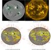Fig. 3 a) SDO/HMI and b) AIA images and their respective selected magnetic field lines plots reconstructed from c) SOLIS and d) HMI magnetograms using NLFFF modeling. The color coding shows Br on the photosphere. Yellow field lines represent closed field lines, while field lines changing in color from yellow to brown (from bottom to the top) represent the open ones. The gray area indicates the region where magnetic field values are close to zero.

To study the influence of the use of preprocessed boundary data from the observed boundary fields on the estimation of free-magnetic energy, we have computed the magnetic energy associated with the potential field and NLFFF configurations from the original SDO/HMI data without preprocessing and with preprocessing. The case for SOLIS/VSM has been studied by Tadesse et al. (2012a). As preprocessing procedure filters out small scale surface field fluctuations, the magnetic energy associated with NLFFF obtained from preprocessed SDO/HMI boundary data is weaker than the one without preprocessing. Obviously, the potential field energies of boundary data with and without preprocessing are close in value, since the potential field calculation makes use of the radial magnetic field component which is not affected too much by preprocessing procedure. The computed magnetic energy from SDO/HMI original data without preprocessing is about 9.067 × 10³³   erg, which is about 1.7% higher than the one obtained from preprocessed and modified observational HMI boundary data. However, this energy does not correspond to the nonlinear force-free magnetic field solution since the original boundary data without preprocessing is not a consistent boundary condition for NLFFF modeling (Tadesse et al. 2012a).

Fig. 4 Magnetic pressure pm in the longitudinal cross-section at θ = 20° for the a) VSM and b) HMI. The vertical and horizontal axes show radial distance in solar radius and longitude, φ on the photosphere, respectively.

Fig. 5 Vector plot of the radial component of electric current density and vector field plot of transverse component of electric current density with white arrows. The colour coding shows Jr on the photosphere. The vertical and horizontal axes show latitude, θ and longitude, φ on the photosphere respectively.

We investigated the magnetic field configurations of the VSM and HMI models by comparing the vector components. We calculated the vector correlation (using Eq. (6) in the computational volume) of the potential fields and the NLFFF fields. The average vector correlation between the potential fields based on the HMI and VSM data is 0.97. The average vector correlation between the NLFFF fields of HMI and VSM data is 0.94. Figures 3a and b. show the surface radial magnetic field component observed by HMI instrument on November 09 2011 and the corresponding AIA (Atmospheric Imaging Assembly) image in 171 Å, respectively. The magnetic field lines obtained from NLFFF extrapolation based on HMI and VSM data have good correlations as shown in Figs. 3c and d, with the foot points of the field lines from the two magnetograms are identical. However, there are some differences. For example, extrapolated field lines from SDO/HMI magnetogram (Fig. 3d) do not show transequatorial loops connecting trailing polarity of NOAA AR 11339 (west of central meridian in northern hemisphere) and trailing polarity of AR11338 (southern hemisphere). This transequatorial loop is well represented by NLFFF extrapolation based on SOLIS/VSM. This difference can be attributed to presence of a patch of weak fields between two active regions (in SDO/HMI data). With this weak field patch, SDO/HMI model tends to close field lines originating in trailing polarity of AR11339, while SOLIS/VSM model extends them to AR11338. Both extrapolations indicate loops connecting AR11339 and AR11342 (East of central meridian in Northern hemisphere). Although SDO/AIA image (Fig. 3b) does not show coronal loops connecting these two active region, such loops are clearly visible in images taken by X-ray Telescope on Hinode. These loops appear to fit better field lines from SOLIS/VSM model. Despite a relatively good visual agreement in extrapolated fields, the models show some notable disagreement in derived magnetic energy. Thus, for example, the estimated free magnetic energy obtained from SDO/HMI is 14.4% higher than that of SOLIS/VSM. This is due to the fact that HMI data includes small scale magnetic fields measurements. We study the magnetic pressure, p_m, in a longitudinal cross-section at about θ = 20° as shown in Fig. 4. The overall pattern of p_m appears to be the same when calculated from the HMI and VSM NLFFF model volume. In this study we found that the magnetic pressure of NLFFF model field from HMI is greater than that of VSM for same locations in the cross section. This is expected, since the magnetic pressure is proportional to the magnetic energy density as the magnetic energy of NLFFF model field from HMI is greater than that of VSM. The surface radial (J_r) and transverse (J_t) electric current densities of the NLFFF field models based on HMI and VSM data are shown in Fig. 5. The value of the total radial surface electric current density flux of the NLFFF field models based on HMI is greater that than that of VSM. It agrees with fact that the HMI instrument measures more transverse magnetic field than that of VSM instrument. The transverse surface electric current density of the NLFFF field model based on HMI spreads more around the active regions than that of VSM as shown in Fig. 5. This could reflect the fact (see Pietarila et al. 2012) that the scaling factor between SOLIS/VSM and SDO/HMI is different for weak and strong fluxes. This difference is scaling factor may act as a weighting function when comparing electric currents derived from two models. In addition, the vector correlations of the radial and transverse surface electric current densities of the NLFFF field models based on HMI and VSM are 0.96 and 0.88, respectively. This indicate that there is more pronounced discrepancy in transverse electric current densities than radial one.

5. Conclusion and outlook

We have investigated the coronal magnetic field associated with full solar disk on November 09, 2011 by analysing SDO/HMI and SOLIS/VSM data. We carried out nonlinear force-free coronal field extrapolations of a full disk magnetograms. The vector magnetogram is almost perfectly flux balanced and the field of view was large enough to cover all the weak field surrounding the active regions. Both conditions are necessary in order to carry out meaningful force-free computations. We have used the optimization method for the reconstruction of nonlinear force-free coronal magnetic fields in spherical geometry (Wiegelmann 2007; Tadesse et al. 2009) to campare the final NLFFF model field solution from HMI and VSM full disk data.

We have found that the optimal value for smoothing parameter is μ₄ = 0.05 for full-disk HMI data for the purpose of preprocessing. We conclude that the choice ν = 0.001 is the optimal choices for HMI full disk data set for our new code as investigated in Wiegelmann et al. (2012).

The magnetic field lines obtained from NLFFF extrapolation based on HMI and VSM data have good correlations. However, the models show some disagreement on the estimated relative free magnetic energy which can be released during explosive events and surface electric current density. Reconstructed magnetic field based on SDO/HMI data have more contents of total magnetic energy, free magnetic energy, the longitudinal distribution of the magnetic pressure and surface electric current density compared to SOLIS/VSM data. Since the disagreement in free energy can be attributed to presence of weaker transverse fields in SDO/HMI measurements, it is not clear how important is the found (14.4%) difference in free magnetic energy for flare and CME processes originating in magnetic fields higher in the corona. This aspect deserves a separate study.

Acknowledgments

The authors thank the anonymous referee for helpful comments. Data are courtesy of NASA/SDO and the AIA and HMI science teams. SOLIS/VSM vector magnetograms are produced cooperatively by NSF/NSO and NASA/LWS. The National Solar Observatory (NSO) is operated by the Association of Universities for Research in Astronomy, Inc., under cooperative agreement with the National Science Foundation. This work was supported by NASA grant NNX07AU64G and the work of T. Wiegelmann was supported by DLR-grant 50 OC 453 0501.

References

All Tables

All Figures

	Fig. 1 Magnetic vector maps of VSM and HMI on part of the lower boundary. The color coding shows Br on the photosphere and the white arrow indicates the transverse components of the field. The vertical and horizontal axes show latitude, θ and longitude, φ on the photosphere respectively.
In the text

	Fig. 2 Mask function for magnetic vector field distribution on full disk from a) VSM and b) HMI. The vertical and horizontal axes show latitude, θ and longitude, φ on the photosphere respectively.
In the text

Fig. 3 a) SDO/HMI and b) AIA images and their respective selected magnetic field lines plots reconstructed from c) SOLIS and d) HMI magnetograms using NLFFF modeling. The color coding shows Br on the photosphere. Yellow field lines represent closed field lines, while field lines changing in color from yellow to brown (from bottom to the top) represent the open ones. The gray area indicates the region where magnetic field values are close to zero.

In the text

	Fig. 4 Magnetic pressure pm in the longitudinal cross-section at θ = 20° for the a) VSM and b) HMI. The vertical and horizontal axes show radial distance in solar radius and longitude, φ on the photosphere, respectively.
In the text

	Fig. 5 Vector plot of the radial component of electric current density and vector field plot of transverse component of electric current density with white arrows. The colour coding shows Jr on the photosphere. The vertical and horizontal axes show latitude, θ and longitude, φ on the photosphere respectively.
In the text

References

- Aly, J. J. 1989, Sol. Phys., 120, 19 [NASA ADS] [CrossRef] [Google Scholar]
- Amari, T., & Aly, J. 2010, A&A, 522, A52 [NASA ADS] [CrossRef] [EDP Sciences] [Google Scholar]
- Amari, T., Aly, J. J., Luciani, J. F., Boulmezaoud, T. Z., & Mikic, Z. 1997, Sol. Phys., 174, 129 [NASA ADS] [CrossRef] [Google Scholar]
- Amari, T., Boulmezaoud, T. Z., & Mikic, Z. 1999, A&A, 350, 1051 [NASA ADS] [Google Scholar]
- Amari, T., Boulmezaoud, T. Z., & Aly, J. J. 2006, A&A, 446, 691 [NASA ADS] [CrossRef] [EDP Sciences] [Google Scholar]
- Aschwanden, M. J. 2008, JA&A, 29, 115 [NASA ADS] [Google Scholar]
- Auer, L. H., House, L. L., & Heasley, J. N. 1977, Sol. Phys., 55, 47 [NASA ADS] [CrossRef] [Google Scholar]
- Borrero, J. M., Tomczyk, S., Kubo, M., et al. 2011, Sol. Phys., 273, 267 [Google Scholar]
- Canou, A., & Amari, T. 2010, ApJ, 715, 1566 [NASA ADS] [CrossRef] [Google Scholar]
- Canou, A., Amari, T., Bommier, V., et al. 2009, ApJ, 693, L27 [NASA ADS] [CrossRef] [Google Scholar]
- DeRosa, M. L., Schrijver, C. J., Barnes, G., et al. 2009, ApJ, 696, 1780 [Google Scholar]
- Gary, G. A. 2001, Sol. Phys., 203, 71 [NASA ADS] [CrossRef] [Google Scholar]
- Georgoulis, M. K. 2005, ApJ, 629, L69 [NASA ADS] [CrossRef] [Google Scholar]
- Guo, Y., Ding, M. D., Schmieder, B., et al. 2010, ApJ, 725, L38 [NASA ADS] [CrossRef] [Google Scholar]
- Inhester, B., & Wiegelmann, T. 2006, Sol. Phys., 235, 201 [NASA ADS] [CrossRef] [Google Scholar]
- Jiang, C., & Feng, X. 2012, ApJ, 749, 135 [NASA ADS] [CrossRef] [Google Scholar]
- Jones, H. P., Harvey, J. W., Henney, C. J., Hill, F., & Keller, U. C. 2002, ESA SP, 505, 15 [Google Scholar]
- Keller, U. C., Harvey, J. W., & Giampapa, M. S. 2003, 4853, 194 [Google Scholar]
- Leka, K. D., Barnes, G., Crouch, A. D., et al. 2009, Sol. Phys., 260, 83 [Google Scholar]
- Metcalf, T. R. 1994, Sol. Phys., 155, 235 [Google Scholar]
- Metcalf, T. R., Leka, K. D., Barnes, G., et al. 2006, Sol. Phys., 237, 267 [Google Scholar]
- Metcalf, T. R., De Rosa, M. L., Schrijver, C. J., et al. 2008, Sol. Phys., 247, 269 [Google Scholar]
- Molodensky, M. M. 1969, SvA-AJ, 12, 585 [Google Scholar]
- Pietarila, A., Bertello, D., Harvey, F., & Pevtsov, A. 2012, Sol. Phys., 256 [Google Scholar]
- Régnier, S., & Amari, T. 2004, 425, 345 [Google Scholar]
- Régnier, S., & Priest, E. R. 2007a, A&A, 468, 701 [NASA ADS] [CrossRef] [EDP Sciences] [Google Scholar]
- Régnier, S., & Priest, E. R. 2007b, ApJ, 669, L53 [NASA ADS] [CrossRef] [Google Scholar]
- Régnier, S., Amari, T., & Kersalé, E. 2002, A&A, 392, 1119 [NASA ADS] [CrossRef] [EDP Sciences] [Google Scholar]
- Ronan, R. S., Mickey, D. L., & Orrall, F. Q. 1987, Sol. Phys., 113, 353 [NASA ADS] [CrossRef] [Google Scholar]
- Sandman, A. W., & Aschwanden, M. J. 2011, Sol. Phys., 270, 503 [NASA ADS] [CrossRef] [Google Scholar]
- Schou, J., Scherrer, P. H., Bush, R. I., et al. 2012, Sol. Phys., 275, 229 [Google Scholar]
- Schrijver, C. J. 2009, Adv. Space Res., 43, 739 [NASA ADS] [CrossRef] [Google Scholar]
- Schrijver, C. J., & Title, A. M. 2011, J. Geophys. Res., 116, A04108 [Google Scholar]
- Schrijver, C. J., Derosa, M. L., Metcalf, T. R., et al. 2006, Sol. Phys., 235, 161 [Google Scholar]
- Skumanich, A., & Lites, B. W. 1987, ApJ, 322, 473 [Google Scholar]
- Tadesse, T., Wiegelmann, T., & Inhester, B. 2009, A&A, 508, 421 [NASA ADS] [CrossRef] [EDP Sciences] [Google Scholar]
- Tadesse, T., Wiegelmann, T., Inhester, B., & Pevtsov, A. 2011, A&A, 527, A30 [NASA ADS] [CrossRef] [EDP Sciences] [Google Scholar]
- Tadesse, T., Wiegelmann, T., Inhester, B., & Pevtsov, A. 2012a, Sol. Phys., 281, 53 [NASA ADS] [Google Scholar]
- Tadesse, T., Wiegelmann, T., Inhester, B., & Pevtsov, A. 2012b, Sol. Phys., 277, 119 [NASA ADS] [CrossRef] [Google Scholar]
- Thalmann, J. K., Wiegelmann, T., & Raouafi, N.-E. 2008, A&A, 488, L71 [NASA ADS] [CrossRef] [EDP Sciences] [Google Scholar]
- Thalmann, J. K., Pietarila, A., Sun, X., & Wiegelmann, T. 2012, AJ, 144, 33 [Google Scholar]
- Turmon, M., Jones, H. P., Malanushenko, O. V., & Pap, J. M. 2010, Sol. Phys., 262, 277 [NASA ADS] [CrossRef] [Google Scholar]
- Unno, W. 1956, Publ. Astron. Soc. Japan, 8, 108 [Google Scholar]
- Valori, G., Kliem, B., & Keppens, R. 2005, A&A, 433, 335 [NASA ADS] [CrossRef] [EDP Sciences] [Google Scholar]
- Valori, G., Green, L. M., Démoulin, P., et al. 2012, Sol. Phys., 278, 73 [NASA ADS] [CrossRef] [Google Scholar]
- Wheatland, M. S. 2004, Sol. Phys., 222, 247 [NASA ADS] [CrossRef] [Google Scholar]
- Wheatland, M. S., & Leka, K. D. 2011, ApJ, 728, 112 [NASA ADS] [CrossRef] [Google Scholar]
- Wheatland, M. S., & Régnier, S. 2009, ApJ, 700, L88 [NASA ADS] [CrossRef] [Google Scholar]
- Wheatland, M. S., Sturrock, P. A., & Roumeliotis, G. 2000, ApJ, 540, 1150 [Google Scholar]
- Wiegelmann, T. 2004, Sol. Phys., 219, 87 [NASA ADS] [CrossRef] [Google Scholar]
- Wiegelmann, T. 2007, Sol. Phys., 240, 227 [NASA ADS] [CrossRef] [Google Scholar]
- Wiegelmann, T., & Inhester, B. 2010, A&A, 516, A107 [NASA ADS] [CrossRef] [EDP Sciences] [Google Scholar]
- Wiegelmann, T., Inhester, B., & Sakurai, T. 2006, Sol. Phys., 233, 215 [NASA ADS] [CrossRef] [Google Scholar]
- Wiegelmann, T., Thalmann, J. K., Inhester, B., et al. 2012, Sol. Phys., 281, 37 [NASA ADS] [Google Scholar]
All Tables
Flux-balance, force and torque free parameters of SOLIS/VSM and SDO/MHI full disk magnetograms.
Magnetic energy associated with extrapolated NLFFF field configurations from full disk SDO/HMI and SOLIS/VSM data.