| Issue |
A&A
Volume 659, March 2022
|
|
|---|---|---|
| Article Number | A174 | |
| Number of page(s) | 11 | |
| Section | The Sun and the Heliosphere | |
| DOI | https://doi.org/10.1051/0004-6361/202038001 | |
| Published online | 23 March 2022 | |
Coronal magnetic field evolution over cycle 24
1
Max-Planck-Institut für Sonnensystemforschung, Justus-von-Liebig-Weg 3, 37077 Göttingen, Germany
e-mail: chifu@mps.mpg.de
2
Institute of Astrophysics and Geophysics, University of Göttingen, Friedrich-Hund-Platz 1, 37077 Göttingen, Germany
Received:
22
March
2020
Accepted:
27
December
2021
Context. The photospheric magnetic field vector is continuously derived from measurements, while reconstruction of the three-dimensional (3D) coronal magnetic field requires modelling with photospheric measurements as a boundary condition. For decades, the cycle variation of the magnetic field in the photosphere has been investigated. Until now, there has been no study of the evolution of the coronal magnetic flux in the corona or of the evolution of solar cycle magnetic free energy.
Aims. The aim of this paper is to analyze the temporal variation of the magnetic field and free magnetic energy in the solar corona for solar cycle 24 and the behavior of the magnetic field in the two hemispheres. We want to investigate whether or not we can obtain better estimates of the magnetic field at Earth using the nonlinear force-free field extrapolation method.
Methods. To model the magnetic field over cycle 24 we apply the nonlinear force-free field (NLFFF) optimization method to the entire set of the synoptic vector magnetic maps derived from observations made using the Heliospheric and Magnetic Imager (HMI) on board Solar Dynamic Observatory (SDO).
Results. From our results, we find that during solar cycle 24, the maximum of the Sun’s dynamics is different than the sunspot number (SSN) maximum peak. The major contribution to the total unsigned flux is provided by the flux coming from the magnetic field structures other than sunspots (MSOS) within latitudes of −30° and +30°. The magnetic flux variation during solar cycle 24 shows a different evolution in the corona than in the photosphere. We find a correlation value of 0.8 between the derived magnetic energy from our model and the flare energy index derived from observations. On average, cycle 24 had a higher number of sunspots in the northern hemisphere (NH) but stronger flux in the southern hemisphere (SH) which could more effectively reach the higher layers of the atmosphere. The coupling between the hemispheres increases with height. The strongest asymmetries in the unsigned magnetic flux are between the two SSN peaks.
Key words: Sun: activity / Sun: corona / Sun: evolution / Sun: magnetic fields
© I. Chifu et al. 2022
 Open Access article, published by EDP Sciences, under the terms of the Creative Commons Attribution License (https://creativecommons.org/licenses/by/4.0), which permits unrestricted use, distribution, and reproduction in any medium, provided the original work is properly cited.
Open Access funding provided by Max Planck Society.
1. Introduction
In 1843, the German astronomer Schwabe discovered the 11-year solar cycle. A few years later, Wolf compiled Schwabe’s observations of sunspots with other observations dating back to Galileo’s first recordings. Based on Wolf’s numbering, cycle number one falls into the period 1755–1766. The connection between the solar cycle and a variation in the Sun’s magnetic activity was only recognised at the beginning of the 20th century by the American astronomer Hale (see Hathaway 2010, for a review paper).
Investigating the cycle variation in more detail, it was found that the SSN for many maxima displays a double peak known as the Gnevyshev peak (Gnevyshev 1977, 1963; Karak et al. 2018). The period between the two peaks is known as the Gnevyshev gap. It was noted that the two peak phenomena seem to appear in both hemispheres (Norton & Gallagher 2010; Temmer et al. 2006). One possible explanation was suggested by Karak et al. (2018) based on dynamo simulations. The authors conclude that the double peaks of one cycle are due to surges of opposite polarity in the polar surface magnetic field observed in the previous cycle. The global magnetic field variation during a solar cycle can be related to the coupling between the northern and southern hemispheres, and the coupling strength then determines the phase-lag between them (Norton & Gallagher 2010).
The effects of the solar cycle in the corona did not receive as much attention as those in the photosphere. The main reason for this difference is probably the difficulty in measuring the magnetic field in the corona. While the vector magnetic field in the photosphere is derived from daily observations made by HMI/SDO, the magnetic field in the corona has occasionally been derived from direct measurements. Instead, an estimate of the coronal magnetic field can be obtained through extrapolation from the magnetic field in the photosphere.
The variation of the sunspot activity during the solar cycle certainly has an impact on the solar corona. The strong magnetic flux from larger sunspots shapes the magnetic field in most of the corona. The contribution from numerous small-scale flux concentrations in quiet Sun surface regions is less obvious (Lagg et al. 2010). While the effect of the concentrated flux in the sunspots can be clearly seen in the extreme ultra-violet (EUV) coronal images, the effect of the flux from smaller regions is not as visible in the corona. The data of reduced spacial scale used as input in the NLFFF extrapolations do not allow us to see if there are any effects in the corona due to small-area photospheric magnetic flux concentrations.
One of the few investigations of the solar cycle variations in the corona deals with the temperature and emission measure using EUV data from 2010–2017; see Morgan & Taroyan (2017). The authors compared these thermal plasma properties with variations in the surface magnetic field and concluded that their analysis could be improved if the comparison was made with the coronal magnetic field modeled over long time periods of for example a solar cycle.
In this paper, we pick up the suggestion by Morgan & Taroyan (2017) and model the coronal magnetic field for the entirety of solar cycle 24. To our knowledge, there has been no comparable investigation of the temporal evolution of the magnetic flux and magnetic energy in the solar corona during an entire solar cycle. We consider the above quantities in each hemisphere separately to see how the hemispheric balance changes from photosphere to the corona.
Solar cycle 24 appears to be the weakest compared with the previous four cycles, which were already weak. Janardhan et al. (2018) reports an unusual polar field reversal during cycle 24. The extent to which our results can be generalised to previous solar cycles is therefore unclear.
The paper is structured as follows: in Sect. 2, we briefly describe the extrapolation method used for deriving the coronal magnetic field; in Sect. 3, we describe the data and the setup of the extrapolation. The results are presented in Sect. 4, followed by discussions and conclusions in Sect. 5.
2. The coronal magnetic field extrapolation method
A basic assumption of the extrapolation method is the stationarity of the coronal magnetic field and its photospheric boundary on scales larger than the spatial resolution of the field model and on temporal scales longer than an Alfven transit time through the model domain. Both these assumptions hold because the spatial and temporal scales we consider in this study are large, a fraction of the solar radius and a fraction of the 11-year cycle, respectively. The other major assumption is that nonmagnetic forces such as thermal and dynamic pressure and gravitational forces can be neglected. The ratio of the thermal pressure to the magnetic pressure is expressed by the plasma beta parameter (β). According to a study by Gary (2001), in the corona, the magnetic pressure dominates the plasma pressure over a large range of coronal altitudes. Gravitational forces and dynamic pressure can be neglected on the scales considered here where the gravitational escape speed and the plasma flow speed stay well below the Alfven speed.
For a review of global coronal magnetic field extrapolations, including a discussion of the effects of neglecting terms from a full magnetohydrodynamic (MHD) model effect, can be found in Wiegelmann et al. (2017). The work done in the present paper is based on global NLFFF extrapolations. A source for evaluating both the problems and achievements of NLFFF on global scales in comparison with other nonpotential global models is the study by Yeates et al. (2018). In this latter paper, which was based on two ISSI1 meetings, seven different global nonpotential codes (two NLFFF codes, magnetohydrostatics (MHS), force-free electrodynamics, magneto frictional, MHD, and zero-beat MHD) were applied to model the solar corona during the solar eclipse from March 2015, and the results were compared. The authors found that in all investigated models, some details match with observations, while others do not. A main reason for this is related to the distribution of electric currents, because currents are a key aspect regarding the nonpotentiality of the coronal magnetic field. It was concluded that the NLFFF extrapolations perform best in active regions (ARs) where reliable vector magnetic fields are measured. Such data are not available outside ARs and to compute the free energy here requires time-evolving models, as in for example the magneto-frictional approach. As a result, the global NLFFF approach is likely to underestimate the amount of free energy, because it neglects energy sources outside ARs. Peter et al. (2015) questioned the assumption that the plasma β is orders of magnitudes lower than unity in the corona, a basic assumption of the NLFFF extrapolations. By performing MHD simulations, which are also an approximation, the authors concluded that the low plasma β assumption in the corona does not hold, and plasma β can be larger than 0.1. The authors further concluded that neglecting the finite-beta effects in NLFFF makes estimations of the free magnetic energy unreliable if the plasma β is of the order of the free energy. This effect is strongest for ARs with relatively small free energy (5%−10% of the potential field energy). For ARs with strong parallel electric currents and high relative magnetic energy, the effect becomes weaker. Another effect is that the spatial resolution of the computation is important, and higher resolution computations show more free magnetic energy (see DeRosa et al. 2015, for details). As a consequence, these three effects (missing vector magnetograms in the quiet Sun, neglecting finite-beta effects, limited spatial resolution) cause an underestimation of the free magnetic energy in global NLFFF models. The free energies deduced from these models can be considered as a lower limit on the magnetic energy. Nevertheless, despite these shortcomings, the amount of energy computed from NLFFF is a useful quantity. Simpler potential field source surface models have a free magnetic energy of zero by construction and even if NLFFF models provide only a lower limit on the access energy, this can give some insight into the energy sources available for the activity of the Sun. De Rosa et al. (2009) address the limitation of NLFFF methods when applied to an AR in a small computational box and they suggested that the extrapolation of an AR should be performed using a much larger field of view (FOV) around the target. Such data are now (since 2010) available from SDO/HMI and the global computations based on synoptic vector maps have the largest possible FOV. It was also pointed out that the NLFFF codes should incorporate measurement errors in the vector fields, which current state-of-the-art NLFFF codes do. Another identified issue was that the traced magnetic field lines from the solution of the extrapolation do not always perfectly match the observations and that the photosphere-corona interface is not well understood. Progress regarding a better modelling of this forced interface region has been done with a MHS model; see for example Zhu et al. (2020). MHS models take nonmagnetic forces and finite-beta effects into account self-consistently, but for a physical understanding of the thin layer between photosphere and corona, very high-resolution vector magnetograms are required and MHS models need a much longer computing time than NLFFF. Currently, the resolution of the available synoptic vector magnetograms is not sufficient and consequently this approach is still not feasible for global models. For more details about force-free coronal magnetic fields, see the review papers by Wiegelmann & Sakurai (2012, 2021).
The extrapolation method we use was initially proposed by Wheatland et al. (2000) and implemented by Wiegelmann (2004). It is described in detail in Wiegelmann (2007) and so we only mention the special variant that we used for this study. The method is based on the force-free field assumption, that is, the Lorentz force j × B = 0 vanishes together with ∇ ⋅ B = 0. This assumption is an idealization as it implies stationarity and the vanishing of pressure and gravity forces. The coronal field B in domain V is obtained by simultaneously minimising the three integral terms from the functional L = L1 + L2 + L3, where

which intend to cause the resulting field to be force-free (term L1), divergence-free (term L2) and to match the photospheric boundary observations Bobs (term L3). Here, wd is a space-dependent weight which tapers the lateral and top boundaries (see Wiegelmann 2004, for more details), and  is the space-dependent variance of the measurement error in the surface field Bobs at the bottom boundary S of V (see Tadesse et al. 2014, for more details).
One of the main assumptions of the force-free magnetic field modeling is that the plasma β is much – or at least one order of magnitude – lower than unity. In the corona, this assumption is valid (see Gary 2001), but in the photosphere, plasma β is of the order of unity. According to Wiegelmann et al. (2006) (and the references therein), a vector magnetogram fulfils the force-free assumption if the total flux, force, and torque are much lower than unity (see Tadesse 2011, for the expression of these quantities). If this condition is not fulfilled, one should apply preprocessing on the vector magnetograms (Wiegelmann et al. 2006; Tadesse 2011). Wiegelmann et al. (2012) checked the consistency of the HMI vector magnetogram with the force-free assumption by calculating the expressions of force, torque, and flux. For the evaluation, the authors used a FOV comprised of an AR and its surroundings but not the entire vector magnetogram. They concluded that for the investigated data set, the HMI vector magnetograms do not need preprocessing because the values of the force, torque, and flux were of the order of 10−2, 10−3, respectively. Nevertheless, one should always check the consistency of the boundary data.
The computational domain V extends over r = [1, 2.5] solar radius (Rs) in the heliocentric radial direction, θ = [ − 70° ,70° ] in latitude, and ϕ = [0° ,360° ] in longitude. At altitudes beyond 2.5 Rs, the plasma β increases toward unity and dynamic forces can no longer be neglected as the solar wind bulk velocity approaches the Alfvèn speed. The latitudinal boundaries exclude the pole areas because the surface data in polar latitudes are of poor quality and the numerical finite-difference representation we use for the integrals in Eqs. (1)–(3) becomes singular at the poles. The method uses the observed vector magnetogram as the bottom boundary. The lateral and top boundaries are fixed from an initially calculated potential field.
The NLFF field reconstructions are calculated iteratively from an initial magnetic field until the field B has relaxed to a force-free state. We use the multiscale approach. On the coarsest grid of 45 × 70 × 180 in r × θ × ϕ, we use an initial potential field determined from the normal component of the surface field. The solution of the NLFFF extrapolation, on all but the finest grid, is interpolated on the next grid and used as the initial condition for the extrapolation on the new grid. The final coronal field model analyzed below is the result obtained on the 180 × 280 × 720 grid. At any level change, the grid size is reduced (enhanced) by a factor of two.
3. The data
As the bottom boundary input for the NLFFF extrapolation, we used vector magnetic field data from the HMI instrument on board SDO (Pesnell et al. 2012). One of the data products suitable for the full Sun extrapolation provided by the HMI team (Liu et al. 2017) is the synoptic maps which are derived from the daily HMI vector magnetograms. Each longitude stripe from the synoptic map represents the average of 20 magnetograms obtained at the central meridian passage of that longitude. The size of the HMI synoptic magnetograms is 3600 × 1440 pixels and the pixel size is 0.1 deg in longitude and 0.001 in sin latitude.
We used the synoptic data from June 2010 to August 2019, which corresponds to Carrington rotation (CR) 2097 to 2220. Figure 1 shows a sample of a synoptic vector magnetogram for CR 2103.
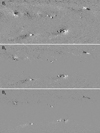 |
Fig. 1. HMI synoptic vector magnetogram for the CR 2103 showing all of the three components of the magnetic field with the Br component displayed on top, Bθ in the middle, and Bϕ at the bottom. |
For verifying the consistency of the boundary data with the force-free assumption, we evaluated the flux, force, and torque for all of the synoptic maps used. While the values obtained for torque are comparable with the one by Wiegelmann et al. (2012), the values for flux and force are in some cases one order of magnitude higher but are still sufficiently low.
4. Results
The magnetic activity is highly influenced by the appearance of the strong concentrations of magnetic flux, which can take the shape of sunspots, faculae, and inter-granular high flux concentrations.
A good proxy for the temporal evolution of the magnetic activity of a cycle is represented by the SSN within that cycle. Using the daily total SSN database of the World Data Center (WDC) – Sunspot Index and Long term Solar Observations (SILSO) updated by the Royal Observatory of Belgium (ROB), we derived the SSN for each CR between June 2010 (CR 2097) and August 2019 (CR 2220). Figure 2 shows the running average over the four CRs of the total SSN (solid black line), and the northern (dashed red line) and southern (dash-dotted blue line) hemisphere contributions.
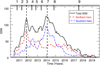 |
Fig. 2. Sunspot number variation during solar cycle 24. Running average over the four CRs is shown with a solid black line for the total SSN, with a dashed red line for the NH, and with a dash-dotted blue line for the SH. The vertical marks numbered from 1 to 9 show points of interest, which are described in the main text. Data source: WDC-SILSO, ROB, Brussels. |
For all of the figures, we set points of interest and marked them. Marks 1 and 2 show the tip of an oscillatory pattern during the ascending phase of the cycle. The dashed vertical lines 3 and 7 mark the sunspot cycle peaks, also known as Gnevyshev peaks, identified as the highest values in the SSN data averaged over four CRs. Each hemisphere has its Gnevyshev peaks, that is, numbers 3 and 5 for the NH, and 4 and 7 for the SH. Mark 6 is part of the Gnevyshev gap in the total SSN. Mark 8 shows the solar cycle maximum; it is not identifiable as a maximum in the evolution of the SSN (Fig. 2), but it shows a clear maximum in the variation of the magnetic flux at Sun and Earth in the free energy and flare index. Mark 9 is the last remarkable rise in the cycle activity which is not clearly visible in the SSN variation but is more prominent in the variation of the magnetic flux.
The variation of the magnetic flux gives more detailed information about the evolution of the magnetic activity of the cycle than the variation of the SSNs. Using the HMI radial magnetic field, we calculated the temporal variation of the total unsigned magnetic flux,
in the photosphere (r = 1 Rs), and we derived the total unsigned flux, Φr (Fig. 5), at various heights above the photosphere (r = 1…2.5 Rs) based on the NLFFF solutions. For the flux calculations, we differentiate between five latitudinal regions (Fig. 3): the southern region (SR) flux (ΦSR) with θ = [ − 70° , − 30°], the center region with θ = [ − 30° ,30°] which is the sunspot latitudinal band during a cycle (Charbonneau 2020), the northern region (NR) flux (ΦNR) with θ = [30° ,70° ] and northern (ΦNH) and southern hemispheres (ΦSH) with θ = [ ± 70° ,0° ]. We separate the center region in sunspot umbra flux (ΦSU), sunspot penumbra flux (ΦSPU), and flux originating from magnetic structures other than sunspots (ΦMSOS). We choose the latitudinal limit of ±70 for comparison with the NLFFF extrapolation.
 |
Fig. 3. HMI radial magnetic field at the CR 2158. The y axis of the image is scaled with the sine of the latitude. The yellow stripes are drawn at ±30° and the black lines are the demarcations for ±70°. The red contour represents UPB. |
In order to calculate the total unsigned magnetic sunspot umbra flux ΦSU, we considered all the photospheric flux larger than 1693 G. We chose this threshold based on previous empirical studies. Using HINODE data, Jurčák et al. (2018) found the sunspot umbra–penumbra boundary (UPB) has the most probable value of 1867 G. Mullan & MacDonald (2019) point out that Schmassmann et al. (2018), using data from HMI/SDO, report a UPB of 1693 G. As we use HMI/SDO data, we chose the value reported by Schmassmann et al. (2018). As there is no clear separation between the penumbra and the quiet Sun, we use the value from Schlichenmaier & Solanki (2003) as a threshold, which says that the magnetic field reaches 800 G at the outer sunspot boundary. We consider the total unsigned magnetic sunspot penumbra flux (ΦSPU) to be the flux between 800 G and 1693 G.
The unsigned magnetic flux within θ = [ − 30° ,30° ] shows the closest resemblance to the SSN variation, mainly the flux from the sunspots ΦSS, defined as the sum of the flux from the sunspot umbra (ΦSU) and penumbra (ΦSPU) (Fig. 4 panel a, violet dash-dotted curve). A difference with the SSN evolution is seen in the total magnetic flux  and ΦMSOS at mark number 8, which is about six months after the second Gnevyshev peak (mark 7), that is, at the time when SSNs are already in their descending phase. The maximum of the cycle activity in terms of emerging flux occurs at the end of 2014, a different epoch than the SSN maximum. For the entire solar cycle, ΦMSOS was the main contributor to the total flux in the photosphere. The value of the total unsigned flux from sunspots ΦSS is one order of magnitude lower than the ΦMSOS and a factor of two to five lower than the value from N−S regions. A similar result was obtained by Jin & Wang (2019), who reported that the total flux from the inter-network magnetic field is larger than from the sunspots or pores over solar cycle 24. These latter authors used a threshold of 950 G and 1.0 × 10²⁰ Mx to differentiate between sunspot or pore and the rest of the magnetic structures. According to Abramenko et al. (2018) and Nikbakhsh et al. (2019), the ARs variability and total unsigned flux present a good correlation with the SSN variation for cycle 24. In our results, the total unsigned flux variation does not follow the SSN variation. The source of the unsigned flux at mark 8 has its roots not only in the AR flux but also in the MSOS flux.
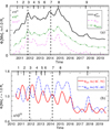 |
Fig. 4. Evolution with time of the photospheric magnetic flux calculated from the HMI data. (a) Evolution of the total photospheric magnetic flux ( |

The unsigned magnetic flux from the northern and southern regions presented in Fig. 4b manifest an anti-phase relationship during most of the cycle, except during the period around mark 9, when the hemispherical regions are almost in phase. The temporal synchronisation has an impact on Φr (Eq. (4)) at each atmospheric level from the photosphere (Fig. 4a) to the corona (Fig. 5).
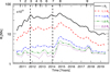 |
Fig. 5. Variation with time of the total unsigned magnetic flux Φri derived from the solution of the NLFFF extrapolation at r = 1.0 Rs (black solid line), 1.1 Rs (dashed red line), 1.5 Rs (dash-dotted blue line), 1.8 Rs (triple dot-dashed green line), and 2.2 Rs (dotted purple line). The flux is shown on a logarithmic scale. |
The beginning of 2016 marks an event in two steps for the evolution of the hemispherical Φr. The first part of the event is visible as a sudden drop in Φr from the northern and southern region (Fig. 4b), seen also in the variation of the total unsigned flux (Fig. 4a). The second part of the event is the beginning of a lower level Φr with respect to the earlier phase of the cycle. From observations, the magnetic flux from the sunspot band diffuses and migrates towards the poles by meridional circulation (Wang et al. 1989). A possible explanation for the first part of the event is that during the migration period, a larger part of the flux canceled and the effect was seen in the unsigned magnetic flux which suffered a sudden drop. A stronger decrease in the SH as observed in Fig. 4b suggests that the sink or cancelation of the magnetic field was more efficient than in the NH.
The second part of the event can probably be explained with the dynamo theory. An important ingredient in the solar dynamo models is the transport of the flux from mid to high latitudes. Some models consider single or multiple-cell meridional circulation which transports the flux from the sunspot band towards the poles. The presence of turbulence gradients in convectively unstable layers give rise to the turbulent pumping mechanism (Guerrero & de Gouveia Dal Pino 2008) which transports the magnetic fields from (near-) surface solar layers to the deep interior (Tobias et al. 1998; Dorch & Nordlund 2001; Ziegler & Rüdiger 2003; Hazra & Nandy 2016). The downward turbulent pumping is considered to be a better mechanism for reducing the polar field strength (Charbonneau 2020). From observations of cycle 23, Hathaway & Rightmire (2010) showed that the meridional flow velocity is higher at solar minimum than SSN maximum. Petrovay (2020) mentions that the overall flow at mid-latitudes is slower before and during maxima, and faster during the decay phase. A faster transport at minimum from the sunspot band to higher latitudes would mean an increase in the unsigned flux above the sunspot band boundary. Cycle 24 observations show that in the descending phase of the cycle there is a decrease in the flux strength within the latitudinal interval of ±30 to ±70 (Fig. 4b). To explain the second part of the event, turbulent pumping might be a solution as considered by Hazra & Nandy (2016). However, we believe such pumping should happen not only at the poles as suggested by Charbonneau (2020). Nandy (2010) considers turbulent pumping to be the most dominant flux transport mechanism for downward transport of the poloidal field. Another possible mechanism explaining the second part of the event is the appearance of multiple meridional circulation cells during the descending phase of the cycle. This would effect the subduction of more magnetic field compared with the previous cycle phase when only one meridional cell would activate.
Over the cycle, the unsigned magnetic flux changes its behaviour with coronal altitudes in respect to the photosphere (Fig. 5). Around the mark labeled number 8, the flux Φri at heights above 1.5 Rs shows an increase by almost a factor of two, much more pronounced than Φri at lower heights. The reason for this increase might be a concentrated strong and complex magnetic field in the photosphere, which has a strong impact on higher layers of the atmosphere.
Figure 6 shows the temporal evolution at r = 1.5, 1.8, and 2.2 Rs of the unsigned Φr from sunspots (right column), MSOS, and northern and southern regions (left column). Except for the NR, all the other components have their highest flux value at mark 8.
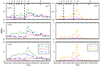 |
Fig. 6. Variation with time of the total unsigned magnetic flux Φri derived from the solution of the NLFFF extrapolation at different heights in the corona. Right panel: evolution of the unsigned flux derived from the solution of the NLFFF extrapolation for the sunspot umbra (solid violet line) and sunspot penumbra (dashed light orange line) within ±30° latitude at heights r = 1.5 (bottom panel), 1.8 (middle panel), and 2.2 (top panel) Rs. Left panel: evolution of the unsigned flux derived from the solution of the NLFFF extrapolation for the magnetic structures other than sunspot umbra (MSOSU) within ±30° latitude (dashed green line) for the NR ΦNR (red dash-dot line) and the SR ΦSR (triple dot-dashed blue line) at heights r = 1.5 (bottom panel), 1.8 (middle panel), and 2.2 (top panel) Rs. |
From the beginning of 2016 until the end of the cycle, the northern and southern regions contribute equal amounts of unsigned flux to the Φr. Starting with the middle of 2017 (Fig. 6, left column), the hemispherical region flux (ΦNR, ΦSR) is higher than the ΦMSOS flux from the sunspot band. On average, over the entire cycle for latitudes between ±30°, the MSOS flux represents around 56% of the total flux in the photosphere and the sunspot flux is around 5%. Cycle 24 had more sunspots in the NH than the SH, but stronger flux in the SH. The NH represents 52 % of the total SSN in Fig. 2. On the other hand, the unsigned flux at the photosphere (Fig. 4b) and corona (Fig. 6, left column) is dominated by the SR, with approximately 53%.
In Fig. 7a we show the normalised asymmetry index for the unsigned magnetic flux at different heights (ΦNH − ΦSH)/(ΦNH + ΦSH) and in Fig. 7b we plot the evolution of the signed magnetic flux from the NH and SH at r = 1.0, 1.5, and 1.8 Rs.
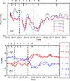 |
Fig. 7. Variation with time of the asymmetry index between NH and SH, and of the signed magnetic flux from the two hemispheres. Panel a: normalized asymmetry flux index for NH and SH, θ = [0° , ± 70° ] derived from the solution of the NLFFF extrapolation at r = 1.0 Rs (dash-dotted black line), 1.5 Rs (dashed blue line), and 1.8 Rs (solid red line). Panel b: signed flux for the NH at r = 1 Rs (thick solid red line), r = 1.5 Rs (dashed red line), and r = 2.2 Rs (dash-dotted red line) and for the SH at r = 1 Rs (thin solid blue line), r = 1.5 Rs (triple dot-dashed blue line), and r = 2.2 Rs (dotted blue line). |
Figure 7a shows, for all heights, the NH flux contributed to the total flux, mainly in the ascending phase, first peak (mark 3), and the second part of the descending phase of the cycle. A small northern flux dominance during the cycle is also noticeable during the Gnevyshev gap (mark 5). The year 2016 marks the beginning of a more symmetric N−S flux for the descending phase of the cycle.
Investigating the SSNs from northern and southern hemispheres of solar cycles 18–23, Temmer et al. (2006) conclude that the hemispheres are in phase during the solar minimum, while high asymmetries beyond statistical uncertainties are noted in the SSN at maximum. The authors report other studies that showed that the N−S asymmetry is higher at solar minimum. From our data, we observe that the N−S asymmetry of the unsigned flux changes with height. In Fig. 7a, strong asymmetries are identified at marks 2, 3, 4–5, 7, and 8 for r = 1.0 Rs, and marks 4–5 and 8 for r = 1.5, 1.8 Rs. Starting with 1.5 Rs, the N−S contribution becomes more symmetric in regions with initial NH dominance. A possible explanation for this is that while in the photosphere the northern emergent flux had its source on larger areas (more sunspots), it was weaker than the southern one, and so it could not penetrate the high layers of the atmosphere as the southern flux could. One of the strong asymmetries (between marks 4 and 5) is co-temporal with an equal number of sunspots from the two hemispheres (Fig. 2) and with the highest amplitude in the SR flux (Fig. 4b). Over all of the atmospheric layers, the strongest asymmetries in the unsigned flux (Fig. 7a) occur during the Gnevyshev gap (between marks 4 and 5) and after the SSN maximum (mark 8).
The hemispheric asymmetry is also an indication of the hemispheric coupling (Antonucci et al. 1990). Analyzing the N−S asymmetry for solar cycles 18–23, Temmer et al. (2006) concluded that the two hemispheres are weakly coupled. According to Antonucci et al. (1990), the time-reversal of the polar fields, the weak interdependence of the magnetic field systems, the level of activity – which differs significantly –, and the asymmetry between the rotation rates from the two hemispheres indicate a weak coupling between the northern and southern hemispheres.
Evaluating the total unsigned magnetic flux (see Fig. 4b), we notice an anti-phase relationship in the photosphere between the two hemispheric regions. At heights above 1.4 Rs (Figs. 6 and 7b), the N−S relation changes with height, and in the top part of the corona, we find that the N and S regions have almost the same level of activity during most of the cycle. From our results (see Figs. 6 and 7a, b), and considering the perspective of Antonucci et al. (1990) on coupling, we observe that, starting from 2016, the two hemispheres become more coupled compared with the previous part of the cycle, and that the coupling between the hemisphere increases with height (Figs. 6 and 7a, b). The correlation between the unsigned flux from the N and S hemispheres increases with height from approximately 0.55 to 0.85.
The observation of the polarity inversion is used as a constraint in the models to predict the evolution and strength of the following solar cycle. In Fig. 7b, we plot the evolution of the magnetic signed flux from the NH and SH at three heights in the atmosphere. Pishkalo (2019), in a study of the photospheric polar (±[50, 90]) magnetic field reversal for the last three cycles, reported multiple reversals in the NH for cycle 24 but just a single SH reversal. These authors published other studies that identify single and multiple reversals in the NH and a single reversal in the SH. From our data, for the photospheric magnetic field within ±[45, 90] we note multiple polarity changes for both hemispheres, while for the field within ±[70, 90] we note single polarity changes in both hemispheres. At heights above 1.5 Rs, the flux (Fig. 7b) has more sign changes than in the photosphere.
Pishkalo (2019) finds that the NH completes the reversal in April 2014 and the SH does this in April–May 2015. Sun et al. (2015a) show that the averaged magnetic field between ±[60, 90] reversed sign in November 2012 (N hem) and in March 2014 (S hem). Janardhan et al. (2018) report that the SH reversed polarity during mid-2013, while the NH started the field reversal as early as June 2012 and completed around November 2014. According to our results, the first change of polarity in the NH (r = 1 Rs) occurs in September–October 2014 (Fig. 7b, solid red line). In agreement with Sun et al. (2015a), we find that the SH changes sign in March–April 2014, an epoch close to the second cycle peak. Janardhan et al. (2018) report different polarity reversal times based on observations made in the low solar corona (17 GHz microwave emission). From our results, we can confirm that the polarity change can also vary with height and not only with time (Fig. 7b). This might be because the differential rotation occurs not only with latitude but also with height and time (Vats et al. 2001; Badalyan 2010). The year 2016 marks the beginning of simultaneous polarity reversals at all atmospheric layers (Fig. 7b) until the end of the cycle.
4.1. Magnetic energy
Most dynamic processes in the corona are driven by the Lorenz forces. As the potential field for a given vertical surface flux distribution in the photosphere has the lowest possible energy, a field configuration involving currents must have excess energy, so-called free energy, if it matches the same photospheric vertical flux distribution. The free energy can therefore serve as a proxy for the probability and the strength of dynamic processes in the corona, such as flares, prominence eruption, or coronal mass ejections (CMEs). Thalmann & Wiegelmann (2008) showed that free energy increases right before a flare eruption and decreases again after the eruption.
We estimate the free energy,
by calculating the actual coronal field BNLFFF through NLFFF extrapolation and determine the potential Bpot using the same vertical surface flux distribution in the photosphere.
In Fig. 8 we show the time evolution of the free energy obtained in the latitudinal range ±70°. Compared to the SSN variation (Fig. 2), we find enhancement at the first major peak at mark 3 (dominated by the northern sunspot) and the first minor peak (dominated by the southern sunspot), the latter with much higher energy. During the second half of the activity cycle, the correlation between SSN and the free energy is poorer. The energy variation shows similarities to the unsigned magnetic flux variation in the corona (Fig. 5), emphasizing the peak at mark 8.
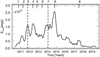 |
Fig. 8. Variation with time of the magnetic free energy obtained from evaluation of the NLFFF magnetic flux. |
In Fig. 9a we display the four-CR running average flare index published by the Kandilli Observatory and Earthquake Research Institute at Bogazici University and made available through the National Oceanic and Atmospheric Administration (NOAA), National Geophysical Data Center (NGDC)2. The flare index is roughly proportional to the mean energy emitted by flares, which is estimated by the product of importance of the flare (see Özgüç et al. 2003, for details) and its duration in minutes. The importance takes into account the area and the intensity of the flare3.
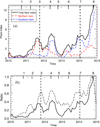 |
Fig. 9. Evolution with time of the flare index, of the total flare index ratio, and free energy ratio. Panel a: variation of the flare index during January 2010 and December 2014: total flare index (solid black line), the contribution from the NH (dashed red line), and from the SH (dash-dotted blue line). Panel b: ratio of the total flare index to its maximum (solid black line) and the ratio of the free energy to its maximum (dash-dotted black line). |
Figure 9b shows the ratios of total flare index to the maximum of the total flare index (solid black line) and of free energy to the maximum of the free energy (dash-dotted black line). We calculated the match between free energy and flare index using Pearson’s correlation coefficient, which gave us a value of 0.88 for the four-CR running averaged curves.
In Fig. 10 we show the four-CR running average of the flare energy. The green dotted curves represent the averages for B class flares while the dashed blue, dash-dotted orange, solid purple curves show the C, M, and X class flares. The figure is constructed based on the data from the Geostationary Operational Environmental Satellite (GOES) through the NOAA NGDC4.
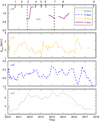 |
Fig. 10. Evolution of the flare energy for the B class (dotted green line), C class (dashed blue line), M class (dash-dotted orange line), and X class (solid purple line) flares. The energy is shown on a logarithmic scale. |
The X-ray flares are classified according to the peak burst intensity measured at the earth in the 1 to 8 angstrom band. There are four classes: the B class flare has an energy peak of less than 10−6 W m−2, the C class has energy of between 10−6 and 10−5 W m−2, M class between 10−5 and 10−4 W m−2, and X class flares between 10−4 and 10−3 W m−2.
In the flare index variation, we identify a first spike shortly before the first solar cycle peak (mark number 3). The free energy (Fig. 9b, dash-dot line) is co-temporal with the first Gnevyshev peak (Fig. 9b, mark number 3) and is not perfectly aligned with the first spike of the flare index (Fig. 9b, solid line). We believe that the free energy peak after the flare index is not the cause of the latter. Previous studies (Thalmann & Wiegelmann 2008) showed an increase in free energy before the occurrence of an AR flare and a decrease in free energy after the eruption. One reason for these phenomena might be that the dependence of the flaring time, which is taken into account when calculating the flare index, is influencing the time variation. While the B class flares follow the unsigned flux variation, including even the oscillatory pattern, the behavior is not present for the C, M, and X class flares. The M class flares show a first energy peak right before mark number 3. These M flares are responsible for the first flare index spike, which appears right before the first cycle peak. We observe the appearance of the X class flares during all SSN peaks, which are prominent in the magnetic flux and energy: the two major peaks, marks 3 and 7, and the first (southern) minor peak, mark 4. In addition, a large number of X class flares are present near the peak marked with the number 8, which can only be seen in magnetic flux and energy. While the strongest flare occurs early in the activity cycle at the first major peak, the highest occurrence rate is at the peak shown by mark 8 during the descending phase of the SSN.
4.2. Magnetic field at Earth
Our estimation of the magnetic field at Earth is based on the open modeled magnetic field in the solar corona at the source surface:
The height at which the coronal field is considered to be “open” is at r = 2.5 Rs, the approximate boundary where the plasma pressure dominates again over the magnetic pressure. Based on the potential field and NLFFF extrapolations, we derived the radial magnetic flux at 1 AU (Eq. (6)).
In Fig. 11a we show the radial component of the observed interplanetary magnetic field at Earth (solid black line), that is, the calculated magnetic field at 1 AU from the NLFFF extrapolation at r = 2.5 Rs (triple dot-dashed red line), r = 2.0 Rs (dashed orange line), and r = 1.8 Rs (dot-dashed violet line). The observed field is from the OMNIWeb5 data center, which is a compilation of data from spacecraft in geocentric or Lagrange one (L1) orbit. Figure 11b shows the ratio between the observed field |Bx| at Earth and that derived with the NLFFF method (|Br1 AU|).
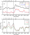 |
Fig. 11. Variation with time of the magnetic field derived from NLFFF and of the magnetic field recorded at 1 AU. Panel a: temporal variation of the observed magnetic field (solid black line) at 1 AU together with the magnetic field derived from the solution of the NLFFF extrapolation at a height of r = 2.5 Rs (triple dot-dashed red line), r = 2.0 Rs (dashed orange line), and r = 1.8 Rs (dot-dashed violet line) and with the magnetic field derived from the potential field at r = 1.8 Rs (dotted blue line). Panel b: ratio between the observed and derived radial unsigned magnetic field at 1 AU. The derived magnetic field was calculated from the solution of the NLFFF at coronal heights of r = 2.5 Rs (dash-dotted black line), r = 2.0 Rs (dotted red line), and r = 1.8 Rs (dashed green line). |
Linker et al. (2017) consider the existence of an “open flux problem” because the calculated flux at Earth based on the open magnetic flux, most often obtained using the potential field source surface (PFSS) method, is much lower than observed flux as in Fig. 11a. Using different magnetograms as bottom boundary for the CR 2098, Linker et al. (2017) modeled the magnetic field in the solar corona using PFSS and MHD methods from which they calculated the magnetic field at Earth. From the solutions of the two methods, these authors obtained the magnetic flux at different heights (r = 1.3, 1.4, 2.0, 2.5 Rs) in the atmosphere from which they calculated the magnetic field at one astronomical unit (1 AU). With one exception (r = 1.3 Rs), the results underestimate the magnetic field at Earth. From our results, the calculation of the magnetic field at 1 AU based on NLFFF extrapolations (Fig. 11) presents the same underestimation expressed by Linker et al. (2017). The magnetic field at Earth based on the solution of the NLFFF is slightly closer to the observations compared to the field obtained from the solution of the potential field. The temporal variation of the magnetic field at 1 AU obtained from in situ measurements (Fig. 11a, solid black line) shows a similar behaviour to the one obtained from extrapolations. By referring to other studies, Linker et al. (2017) argue that one reason for the underestimation of the interplanetary magnetic field values obtained with the models is the appearance of magnetic switchbacks (the behavior of the interplanetary magnetic field to fold back on itself). The consequence is the changing of the magnetic field sign, which will have the effect of an over-counting field value. Linker et al. (2017) analyzed the open flux for one CR at the minimum of activity, and by investigating the sign reversal at Earth they found a total of 88 h of this behavior. Re-evaluating the new observed field, these latter authors obtained a 20% lower value than the recorded one. In the first part of the cycle (from the beginning of our data until mark 7, which coincides with the second SSN peak), we see an underestimation of the calculated field at Earth which might be due to the switchbacks. The lowering of the source surface is not a solution to the discrepancy between the model and the observations; by lowering the source surface to r = 1.8 Rs we obtain a better estimate than for r = 2.5 Rs, but this differs from the folding mechanism and a source-surface below 2 Rs does not agree with field structures concluded from eclipse observations. At the maximum of cycle dynamics (around mark 8) which differs from the indicated maximum of activity in the SSN, we obtain better agreement between the |Bx| and |Br1 AU| compared to the rest of the cycle.
5. Summary and conclusions
We applied the NLFFF optimization method to the HMI vector synoptic maps during solar cycle 24. From the solution of the extrapolation, we calculated the unsigned magnetic flux from photosphere to corona for MSOS and sunspot within latitude θ = [ − 30° ,30° ], for northern (θ = [30° ,70° ]) and southern (θ = [ − 70° ,30° ]) regions and for northern and southern hemispheres (θ = [ ± 70° ,0° ]). The free magnetic energy from the NLFFF model indicates the dynamics in the corona, and the flare index and flare energy reflect the Sun’s dynamics from observations. We calculated the asymmetry index and the signed flux for the N and S hemispheres. In the corona, the N−S contribution becomes more symmetric at the times with an initial high asymmetry (in the photosphere) and NH dominance. The change in symmetry with height might be due to the variation of the differential rotation with height (Vats et al. 2001; Badalyan 2010). From the open magnetic flux maps from the NLFFF solutions at three different heights in the corona (r = 1.4, 1.8, 2.2 Rs), we derive the temporal variation of the magnetic field at 1 AU and compare it with the in situ measurements.
We draw a number of conclusions:
-
The maximum of the cycle activity in terms of emerging flux occurs at the end of 2014, about ten months after the SSN maximum.
-
For the entire solar cycle, ΦMSOS was the main contributor to the total unsigned flux in the photosphere.
-
Cycle 24 had more sunspots in the NH but a stronger unsigned flux in the SH.
-
During the decaying phase of cycle 24, the Φr from the northern and southern regions presents a sudden drop.
-
After the drop, the flux values remain low compared to Φr during the raising and the maximum phase of the cycle.
-
The strongest asymmetries in the unsigned flux occur in all of the atmospheric layers during the Gnevyshev gap (between marks 4 and 5) and after the SSN maximum (mark 8).
-
The coupling between N and S hemispheres increases with height.
-
The polarity change can vary with height and not only with time.
-
The maximum of the free energy at mark 8 indicates that during cycle 24, the maximum occurs ten months later than the maximum in the SSN.
-
The Pearson correlation coefficient between the free energy (calculated from the NLFFF model) and the flare index (calculated from observations) is 0.88.
-
The NLFFF method underestimates the magnetic field at 1 AU but to a slightly lesser extent than PFSS models.
6. Discussions
The first observation from our data is that the Sun had a different magnetic activity maximum during solar cycle 24 (marked number 8 in Figs. 2, 5, 8–11) than the maximum peak of the SSN (mark 7). We support our conclusion with the results obtained from the temporal evolution of the unsigned magnetic flux which gives us the first indication. The magnetic activity peak (mark 8) is also present in the temporal evolution of the free energy, the flare index, and in situ measurements of the magnetic field at Earth. The correlation of 0.88 between the free energy and the flare index gives us confidence that the NLFFF extrapolation provides us with a relatively realistic trend of the solar activity. In the X-ray flare energy data we see that the highest density of the X class flares occurs also in the region marked number 8.
Based on differential emission measure (DEM) profiles, Morgan & Taroyan (2017) created synoptic maps from which they extracted information about temperature (T) and emission measure (EM) in the corona. They compared the T and EM with the radial component of the smoothed photospheric magnetic field. By separating the analysis in the quiet corona and the AR, they conclude that there is no one-to-one correlation between the photospheric magnetic field and the temperature or between the photospheric magnetic field and the emission measure. Figure 3A of Morgan & Taroyan (2017) shows the quiet corona temporal evolution during cycle 24 of |Br|, T, and EM. The temperature has the highest peak immediately before 2015 near the region marked number 8 in our plots where the unsigned magnetic flux (Fig. 5), the free energy (Fig. 8), and the flare index (Fig. 9) have their highest peak. A rigorous comparison between the solution of the magnetic field extrapolation in the corona and the DEM profiles presented by Morgan & Taroyan (2017) might give a better correlation.
The second conclusion that we make based on our results is that the major contribution to the total unsigned flux within the sunspot band latitudes θ ∈ [ − 30° ,30° ] is provided by MSOS. The next important contributors to Φr are the N−S regions (Fig. 4). The total sunspot flux is one order of magnitude lower than the MSOS flux. This result is in agreement with the study of Jin & Wang (2019), even though they made a slightly different classification between the flux sources in sunspots and pores and other magnetic structures. Usually, the dynamo models employ the SSN variation as a reference for the following solar cycle predictions. Including the unsigned magnetic flux activity for these purposes might lead to improved models or predictions.
From the photosphere to the corona, we notice an oscillatory behavior with different frequencies and amplitudes in each of the considered categories (Figs. 2, 4, and 5). The flux activity in sunspots and faculae influences the N−S region oscillations in the unsigned magnetic flux. For example, in Fig. 4 at mark 7 (activity peak in the SSN), we see one of the peaks in the magnetic flux while in the N−S region variation flux we notice low values that are probably the consequence of the Gnevyshev gap (mark 6). The unsigned magnetic MSOS and sunspot flux are contributing to the maximum of the solar cycle dynamics (mark 8) but these probably also contribute to the flux from the N−S regions after it drifted and diffused poleward. On top of this, the superposition of the magnetic shear component over the radial component gives rise to an even further enhanced activity immediately after the SSN peak.
We consider that the reason for the increase in the total unsigned solar and interplanetary magnetic flux visible at mark 8 is the appearance of the AR 12192 in October 2014. This AR contains “the largest sunspot since November 1990”6. For almost ten days, the AR 12192 produced M and X class flares, but it was poor in CMEs (see e.g., Sun et al. 2015b). The effects of its activity were seen at 1 AU for an extended period (Fig. 11).
Linker et al. (2017) suggest a couple of reasons for the underestimation of the magnetic flux at 1 AU calculated from the extrapolation models. One is that the observatory maps systematically underestimate the solar surface magnetic flux. Another argument in favor of underestimation of the interplanetary magnetic field from extrapolations is that, on average, the observed unsigned radial magnetic field is amplified due to switchbacks of the interplanetary magnetic field as suggested by the frequent sign flips of the radial component. The switchbacks would enhance the unsigned flux without changing the total flux average over large sectors (Linker et al. 2017). These presumably transient field irregularities cannot be modeled by a global field extrapolation. If this last mechanism holds, the formation of the folds seems to occur preferentially during the maximum of the SSN. From recent observations by the Parker Solar Probe (Bale et al. 2019), it was found that the switchbacks of the magnetic fields occur already at 36.6 Rs at a minimum of solar activity. When a series of strong events occur, such as the ones triggered by AR 12192, the fold-backs may be destroyed or inhibited by rapidly propagating transients or by an increase in magnetic pressure. The AR 2192 appeared in the SH, and its dissipation had a strong and immediate effect on the unsigned flux from the SR (Fig. 4b, blue curve). In the NR, the dissipation of the unsigned flux was more gentle and occurred at a later time (see the red curves in Fig. 4b).
Acknowledgments
Data are courtesy of NASA/SDO and the HMI science teams. This research was supported by the DFG-grant WI 3211/5-1.
References
- Abramenko, V. I., Zhukova, A. V., & Kutsenko, A. S. 2018, Geomagn. Aeron., 58, 1159 [NASA ADS] [CrossRef] [Google Scholar]
- Antonucci, E., Hoeksema, J. T., & Scherrer, P. H. 1990, ApJ, 360, 296 [Google Scholar]
- Badalyan, O. G. 2010, New Astron., 15, 135 [NASA ADS] [CrossRef] [Google Scholar]
- Bale, S. D., Badman, S. T., Bonnell, J. W., et al. 2019, Nature, 576, 237 [NASA ADS] [CrossRef] [Google Scholar]
- Charbonneau, P. 2020, Liv. Rev. Sol. Phys., 17, 4 [Google Scholar]
- De Rosa, M. L., Schrijver, C. J., Barnes, G., et al. 2009, ApJ, 696, 1780 [NASA ADS] [CrossRef] [Google Scholar]
- DeRosa, M. L., Wheatland, M. S., Leka, K. D., et al. 2015, ApJ, 811, 107 [NASA ADS] [CrossRef] [Google Scholar]
- Dorch, S. B. F., & Nordlund, Å. 2001, A&A, 365, 562 [NASA ADS] [CrossRef] [EDP Sciences] [Google Scholar]
- Gary, G. A. 2001, Sol. Phys., 203, 71 [Google Scholar]
- Gnevyshev, M. N. 1963, Sov. Astron., 7, 311 [NASA ADS] [Google Scholar]
- Gnevyshev, M. N. 1977, Sol. Phys., 51, 175 [NASA ADS] [CrossRef] [Google Scholar]
- Guerrero, G., & de Gouveia Dal Pino, E. M. 2008, A&A, 485, 267 [NASA ADS] [CrossRef] [EDP Sciences] [Google Scholar]
- Hathaway, D. H. 2010, Liv. Rev. Sol. Phys., 7, 1 [Google Scholar]
- Hathaway, D. H., & Rightmire, L. 2010, Science, 327, 1350 [NASA ADS] [CrossRef] [Google Scholar]
- Hazra, S., & Nandy, D. 2016, ApJ, 832, 9 [NASA ADS] [CrossRef] [Google Scholar]
- Janardhan, P., Fujiki, K., Ingale, M., Bisoi, S. K., & Rout, D. 2018, A&A, 618, A148 [NASA ADS] [CrossRef] [EDP Sciences] [Google Scholar]
- Jin, C.-L., & Wang, J.-X. 2019, Res. Astron. Astrophys., 19, 069 [CrossRef] [Google Scholar]
- Jurčák, J., Rezaei, R., González, N. B., Schlichenmaier, R., & Vomlel, J. 2018, A&A, 611, L4 [NASA ADS] [CrossRef] [EDP Sciences] [Google Scholar]
- Karak, B. B., Mandal, S., & Banerjee, D. 2018, ApJ, 866, 17 [CrossRef] [Google Scholar]
- Lagg, A., Solanki, S. K., Riethmüller, T. L., et al. 2010, ApJ, 723, L164 [NASA ADS] [CrossRef] [Google Scholar]
- Linker, J. A., Caplan, R. M., Downs, C., et al. 2017, ApJ, 848, 70 [NASA ADS] [CrossRef] [Google Scholar]
- Liu, Y., Hoeksema, J. T., Sun, X., & Hayashi, K. 2017, Sol. Phys., 292, 29 [NASA ADS] [CrossRef] [Google Scholar]
- Morgan, H., & Taroyan, Y. 2017, Sci. Adv., 3 [CrossRef] [Google Scholar]
- Mullan, D. J., & MacDonald, J. 2019, ApJ, 873, L10 [NASA ADS] [CrossRef] [Google Scholar]
- Nandy, D. 2010, Astrophys. Space Sci. Proc., 19, 86 [NASA ADS] [CrossRef] [Google Scholar]
- Nikbakhsh, S., Tanskanen, E. I., Käpylä, M. J., & Hackman, T. 2019, A&A, 629, A45 [NASA ADS] [CrossRef] [EDP Sciences] [Google Scholar]
- Norton, A. A., & Gallagher, J. C. 2010, Sol. Phys., 261, 193 [NASA ADS] [CrossRef] [Google Scholar]
- Özgüç, A., Ataç, T., & Rybák, J. 2003, Sol. Phys., 214, 375 [CrossRef] [Google Scholar]
- Pesnell, W. D., Thompson, B. J., & Chamberlin, P. C. 2012, Sol. Phys., 275, 3 [Google Scholar]
- Peter, H., Warnecke, J., Chitta, L. P., & Cameron, R. H. 2015, A&A, 584, A68 [NASA ADS] [CrossRef] [EDP Sciences] [Google Scholar]
- Petrovay, K. 2020, Liv. Rev. Sol. Phys., 17, 2 [Google Scholar]
- Pishkalo, M. I. 2019, Sol. Phys., 294, 137 [Google Scholar]
- Schlichenmaier, R., & Solanki, S. K. 2003, A&A, 411, 257 [NASA ADS] [CrossRef] [EDP Sciences] [Google Scholar]
- Schmassmann, M., Schlichenmaier, R., & Bello González, N. 2018, A&A, 620, A104 [NASA ADS] [CrossRef] [EDP Sciences] [Google Scholar]
- Sun, X., Hoeksema, J. T., Liu, Y., & Zhao, J. 2015a, ApJ, 798, 114 [NASA ADS] [CrossRef] [Google Scholar]
- Sun, X., Bobra, M. G., Hoeksema, J. T., et al. 2015b, ApJ, 804, L28 [Google Scholar]
- Tadesse, T. 2011, PhD Thesis, Addis Ababa University [Google Scholar]
- Tadesse, T., Wiegelmann, T., Gosain, S., MacNeice, P., & Pevtsov, A. A. 2014, A&A, 562, A105 [NASA ADS] [CrossRef] [EDP Sciences] [Google Scholar]
- Temmer, M., Rybák, J., Bendík, P., et al. 2006, A&A, 447, 735 [NASA ADS] [CrossRef] [EDP Sciences] [Google Scholar]
- Thalmann, J. K., & Wiegelmann, T. 2008, A&A, 484, 495 [NASA ADS] [CrossRef] [EDP Sciences] [Google Scholar]
- Tobias, S. M., Brummell, N. H., Clune, T. L., & Toomre, J. 1998, ApJ, 502, L177 [NASA ADS] [CrossRef] [Google Scholar]
- Vats, H. O., Cecatto, J. R., Mehta, M., Sawant, H. S., & Neri, J. A. C. F. 2001, ApJ, 548, L87 [NASA ADS] [CrossRef] [Google Scholar]
- Wang, Y. M., Nash, A. G., & Sheeley, N. R., Jr. 1989, Science, 245, 712 [NASA ADS] [CrossRef] [Google Scholar]
- Wheatland, M. S., Sturrock, P. A., & Roumeliotis, G. 2000, ApJ, 540, 1150 [Google Scholar]
- Wiegelmann, T. 2004, Sol. Phys., 219, 87 [NASA ADS] [CrossRef] [Google Scholar]
- Wiegelmann, T. 2007, Sol. Phys., 240, 227 [NASA ADS] [CrossRef] [Google Scholar]
- Wiegelmann, T., & Sakurai, T. 2012, Liv. Rev. Sol. Phys., 9, 5 [Google Scholar]
- Wiegelmann, T., & Sakurai, T. 2021, Liv. Rev. Sol. Phys., 18, 1 [NASA ADS] [CrossRef] [Google Scholar]
- Wiegelmann, T., Inhester, B., & Sakurai, T. 2006, Sol. Phys., 233, 215 [Google Scholar]
- Wiegelmann, T., Thalmann, J. K., Inhester, B., et al. 2012, Sol. Phys., 281, 37 [NASA ADS] [Google Scholar]
- Wiegelmann, T., Petrie, G. J. D., & Riley, P. 2017, Space Sci. Rev., 210, 249 [CrossRef] [Google Scholar]
- Yeates, A. R., Amari, T., Contopoulos, I., et al. 2018, Space Sci. Rev., 214, 99 [CrossRef] [Google Scholar]
- Zhu, X., Wiegelmann, T., & Solanki, S. K. 2020, A&A, 640, A103 [NASA ADS] [CrossRef] [EDP Sciences] [Google Scholar]
- Ziegler, U., & Rüdiger, G. 2003, A&A, 401, 433 [EDP Sciences] [Google Scholar]
All Figures
|
Fig. 1. HMI synoptic vector magnetogram for the CR 2103 showing all of the three components of the magnetic field with the Br component displayed on top, Bθ in the middle, and Bϕ at the bottom. |
| In the text | |
|
Fig. 2. Sunspot number variation during solar cycle 24. Running average over the four CRs is shown with a solid black line for the total SSN, with a dashed red line for the NH, and with a dash-dotted blue line for the SH. The vertical marks numbered from 1 to 9 show points of interest, which are described in the main text. Data source: WDC-SILSO, ROB, Brussels. |
| In the text | |
|
Fig. 3. HMI radial magnetic field at the CR 2158. The y axis of the image is scaled with the sine of the latitude. The yellow stripes are drawn at ±30° and the black lines are the demarcations for ±70°. The red contour represents UPB. |
| In the text | |
|
Fig. 4. Evolution with time of the photospheric magnetic flux calculated from the HMI data. (a) Evolution of the total photospheric magnetic flux ( |
| In the text | |
|
Fig. 5. Variation with time of the total unsigned magnetic flux Φri derived from the solution of the NLFFF extrapolation at r = 1.0 Rs (black solid line), 1.1 Rs (dashed red line), 1.5 Rs (dash-dotted blue line), 1.8 Rs (triple dot-dashed green line), and 2.2 Rs (dotted purple line). The flux is shown on a logarithmic scale. |
| In the text | |
|
Fig. 6. Variation with time of the total unsigned magnetic flux Φri derived from the solution of the NLFFF extrapolation at different heights in the corona. Right panel: evolution of the unsigned flux derived from the solution of the NLFFF extrapolation for the sunspot umbra (solid violet line) and sunspot penumbra (dashed light orange line) within ±30° latitude at heights r = 1.5 (bottom panel), 1.8 (middle panel), and 2.2 (top panel) Rs. Left panel: evolution of the unsigned flux derived from the solution of the NLFFF extrapolation for the magnetic structures other than sunspot umbra (MSOSU) within ±30° latitude (dashed green line) for the NR ΦNR (red dash-dot line) and the SR ΦSR (triple dot-dashed blue line) at heights r = 1.5 (bottom panel), 1.8 (middle panel), and 2.2 (top panel) Rs. |
| In the text | |
|
Fig. 7. Variation with time of the asymmetry index between NH and SH, and of the signed magnetic flux from the two hemispheres. Panel a: normalized asymmetry flux index for NH and SH, θ = [0° , ± 70° ] derived from the solution of the NLFFF extrapolation at r = 1.0 Rs (dash-dotted black line), 1.5 Rs (dashed blue line), and 1.8 Rs (solid red line). Panel b: signed flux for the NH at r = 1 Rs (thick solid red line), r = 1.5 Rs (dashed red line), and r = 2.2 Rs (dash-dotted red line) and for the SH at r = 1 Rs (thin solid blue line), r = 1.5 Rs (triple dot-dashed blue line), and r = 2.2 Rs (dotted blue line). |
| In the text | |
|
Fig. 8. Variation with time of the magnetic free energy obtained from evaluation of the NLFFF magnetic flux. |
| In the text | |
|
Fig. 9. Evolution with time of the flare index, of the total flare index ratio, and free energy ratio. Panel a: variation of the flare index during January 2010 and December 2014: total flare index (solid black line), the contribution from the NH (dashed red line), and from the SH (dash-dotted blue line). Panel b: ratio of the total flare index to its maximum (solid black line) and the ratio of the free energy to its maximum (dash-dotted black line). |
| In the text | |
|
Fig. 10. Evolution of the flare energy for the B class (dotted green line), C class (dashed blue line), M class (dash-dotted orange line), and X class (solid purple line) flares. The energy is shown on a logarithmic scale. |
| In the text | |
|
Fig. 11. Variation with time of the magnetic field derived from NLFFF and of the magnetic field recorded at 1 AU. Panel a: temporal variation of the observed magnetic field (solid black line) at 1 AU together with the magnetic field derived from the solution of the NLFFF extrapolation at a height of r = 2.5 Rs (triple dot-dashed red line), r = 2.0 Rs (dashed orange line), and r = 1.8 Rs (dot-dashed violet line) and with the magnetic field derived from the potential field at r = 1.8 Rs (dotted blue line). Panel b: ratio between the observed and derived radial unsigned magnetic field at 1 AU. The derived magnetic field was calculated from the solution of the NLFFF at coronal heights of r = 2.5 Rs (dash-dotted black line), r = 2.0 Rs (dotted red line), and r = 1.8 Rs (dashed green line). |
| In the text | |
Current usage metrics show cumulative count of Article Views (full-text article views including HTML views, PDF and ePub downloads, according to the available data) and Abstracts Views on Vision4Press platform.
Data correspond to usage on the plateform after 2015. The current usage metrics is available 48-96 hours after online publication and is updated daily on week days.
Initial download of the metrics may take a while.