| Issue |
A&A
Volume 550, February 2013
|
|
|---|---|---|
| Article Number | A106 | |
| Number of page(s) | 14 | |
| Section | Interstellar and circumstellar matter | |
| DOI | https://doi.org/10.1051/0004-6361/201219928 | |
| Published online | 04 February 2013 | |
Low-velocity shocks: signatures of turbulent dissipation in diffuse irradiated gas ⋆
1
ENS, LERMA, UMR 8112, CNRS, LRA/ENS, Observatoire de Paris,
24 rue Lhomond, 75005
Paris, France
e-mail: This email address is being protected from spambots. You need JavaScript enabled to view it.
2
Institut d’Astrophysique Spatiale (IAS), UMR 8617, CNRS,
Université Paris-Sud 11, Bâtiment
121, 91405
Orsay Cedex,
France
3
Departamento de Astrofísica, Centro de Astrobiología, CSIC-INTA,
Torrejón de Ardoz, Madrid, Spain
4
Spitzer Science Center (SSC), California Institute of
Technology, MC
220-6, Pasadena,
CA
91125,
USA
Received: 30 June 2012
Accepted: 5 November 2012
Abstract
Context. Large-scale motions in galaxies (supernovae explosions, galaxy collisions, galactic shear etc.) generate turbulence, which allows a fraction of the available kinetic energy to cascade down to small scales before it is dissipated.
Aims. We establish and quantify the diagnostics of turbulent dissipation in mildly irradiated diffuse gas in the specific context of shock structures.
Methods. We incorporated the basic physics of photon-dominated regions into a state-of-the-art steady-state shock code. We examined the chemical and emission properties of mildly irradiated (G0 = 1) magnetised shocks in diffuse media (nH = 102 to 104 cm-3) at low- to moderate velocities (from 3 to 40 km s-1).
Results. The formation of some molecules relies on endoergic reactions. Their abundances in J-type shocks are enhanced by several orders of magnitude for shock velocities as low as 7 km s-1. Otherwise most chemical properties of J-type shocks vary over less than an order of magnitude between velocities from about 7 to about 30 km s-1, where H2 dissociation sets in. C-type shocks display a more gradual molecular enhancement with increasing shock velocity.
We quantified the energy flux budget (fluxes of kinetic, radiated and magnetic energies) with emphasis on the main cooling lines of the cold interstellar medium. Their sensitivity to shock velocity is such that it allows observations to constrain statistical distributions of shock velocities.
We fitted various probability distribution functions (PDFs) of shock velocities to spectroscopic observations of the galaxy-wide shock in Stephan’s Quintet and of a Galactic line of sight which samples diffuse molecular gas in Chamaeleon. In both cases, low velocities bear the greatest statistical weight and the PDF is consistent with a bimodal distribution. In the very low velocity shocks (below 5 km s-1), dissipation is due to ion-neutral friction and it powers H2 low-energy transitions and atomic lines. In moderate velocity shocks (20 km s-1 and above), the dissipation is due to viscous heating and accounts for most of the molecular emission. In our interpretation a significant fraction of the gas in the line of sight is shocked (from 4% to 66%). For example, C+ emission may trace shocks in UV irradiated gas where C+ is the dominant carbon species.
Conclusions. Low- and moderate velocity shocks are important in shaping the chemical composition and excitation state of the interstellar gas. This allows one to probe the statistical distribution of shock velocities in interstellar turbulence.
Key words: shock waves / astrochemistry / ISM: molecules / ISM: kinematics and dynamics / ISM: abundances
Output data of models are available at the CDS via anonymous ftp to cdsarc.u-strasbg.fr (130.79.128.5) or via http://cdsarc.u-strasbg.fr/viz-bin/qcat?J/A+A/550/A106 and at http://cemag.ens.fr
© ESO, 2013
1. Introduction
Bulk motions in galaxies are generated for instance by supernovae explosions, galaxy collisions and galactic shear. These motions drive turbulence in the cold interstellar medium (ISM). A fraction of the available kinetic energy cascades down to smaller scales and lower velocities. This is spectacularly illustrated by the observations of the galaxy collision in Stephan’s Quintet (SQ). The relative velocities of the galaxies (of about 1000 km s-1) would be expected to dissipate in high-velocity shocks, thus creating a warm and hot plasma devoid of molecules. However, one observes that H2 cooling is greater than the X-ray luminosity (Appleton et al. 2006; Cluver et al. 2010). This demonstrates that energy dissipation in the interstellar space involves an energy cascade and molecular gas cooling. Moreover, the H2 excitation diagram in SQ implies a distribution of temperatures much higher than the equilibrium temperature set by UV and cosmic ray heating. The same holds on much smaller scales in the case of the diffuse ISM in the solar neighbourhood (Gry et al. 2002; Ingalls et al. 2011). The range of gas temperatures can only be accounted for if the dissipation heats the gas through spatially localised events (Falgarone et al. 2005). This idea is also supported by observations of chemical species in the diffuse ISM such as CH+ and SH+, which cannot be reproduced by UV alone (Nehmé et al. 2008; Godard et al. 2012).
These dissipation processes have yet to be studied. Dissipative structures could for instance take the form of shocks, vortices, current sheets, or shear layers and most likely involve the magnetic field. This broad variety of processes, their different time scales and therefore different impacts onto the global gas energetics and chemistry call for simplified models to quantify observational diagnostics. Spectroscopy of molecular H2 with Copernicus in the diffuse ISM motivated the first magnetohydrodynamics (MHD) shock models propagating in diffuse gas. These first models were also the key to provide a first interpretation of CH+ in the diffuse ISM (Mullan 1971; Draine et al. 1983; Flower et al. 1986; Gredel et al. 2002). Observations (Falgarone et al. 2005) by the instrument ISO-SWS of the pure rotational lines of H2 in diffuse gas were also interpreted in the framework of mild turbulent dissipation (low-velocity MHD shocks and/or velocity shears in small-scale vortices). More recently, Godard et al. (2009) have modelled turbulent dissipation bursts in the diffuse ISM as vortices at very small scales and computed the chemical signatures they imprint on the gas.
In the present work, we use an updated version of the magnetised shock models of Flower & Pineau des Forêts (2003) to quantify composition and cooling lines for a range of shock velocities (from 3 to 40 km s-1) including very low velocities that were not thoroughly considered before. We compute grids of these shocks for two strengths of the magnetic field and for three different densities. Our preshock conditions are representative of the cold diffuse ISM. Hence, we have incorporated the treatment of mild irradiation which includes UV heating, but also impacts the chemistry through photo-ionisation and photo-dissociation.
The shock velocity can be a crucial parameter even at very low velocity. Incidentally, the
generation of molecules in the interstellar medium (ISM) is initiated by the formation of
the H2 molecule on dust grains surfaces. Then, the formation of more elaborate
molecules relies on two main paths. One can either add a proton to H2 to form
H and then transfer the extra proton to a
single atom (C, O, S, and Si, with the notable exception of N). But
and then transfer the extra proton to a
single atom (C, O, S, and Si, with the notable exception of N). But
 is usually much less abundant than
H2. Alternatively, one can directly exchange an atom with one proton of the
H2 molecule. But these reactions are subject to energy barriers with high
characteristic temperatures (such as 2980 K in the case of the oxygen atom). Hence both
paths are difficult and the observed molecular complexity of the ISM remains a puzzle.
Nevertheless, temperatures required to open the second path are obtained in low-velocity
shocks (7.5 km s-1 is enough to reach 3000 K). These shocks may therefore play an
important role in shaping the molecular chemistry of the ISM.
is usually much less abundant than
H2. Alternatively, one can directly exchange an atom with one proton of the
H2 molecule. But these reactions are subject to energy barriers with high
characteristic temperatures (such as 2980 K in the case of the oxygen atom). Hence both
paths are difficult and the observed molecular complexity of the ISM remains a puzzle.
Nevertheless, temperatures required to open the second path are obtained in low-velocity
shocks (7.5 km s-1 is enough to reach 3000 K). These shocks may therefore play an
important role in shaping the molecular chemistry of the ISM.
The results of the present models may contribute to interpreting the observations of the full set of cooling lines of the cold neutral medium (CII, CI, OI, H2, CO, and H2O) in galaxies observed with the Spitzer and Herschel space telescopes. To illustrate this, we built models from statistical distributions of shock velocities, which we compared to observed data in SQ and in a line of sight in the Chamaeleon (Gry et al. 2002). We use our best fit models to discuss the impact of kinetic energy dissipation on the physical state and chemistry of the molecular gas in these two sources. We also predict other diagnostic lines to be observed with Herschel.
We present the numerical method for our shock models in Sect. 2, with the properties of our grid of shocks in Sect. 3. In Sect. 4, we use our results to interpret the H2-excitation diagram observed in SQ and Chamaeleon. We summarise and discuss our results in Sect. 5.
2. Numerical method
The models we present in this paper are based on the plane-parallel steady-state shock code implemented in Flower & Pineau des Forêts (2003). We work from their version and include several more refinements mainly to deal with moderate irradiation.
2.1. Radiation
We started from the reactions network used in Flower
& Pineau des Forêts (2003) and included the relevant photo-reactions. The
photo-reactions have rates of the form
 (1)where α and
β are constants. We used an incident field equal to the standard
interstellar radiation field (ISRF, Draine 1978),
thus taking G0 = 1. The extinction
Av is integrated along the model from the
pre-shock where we use a value of
Av = Av0 = 0.1,
which models extinction from the irradation source by a “buffer” of matter. The value of
Av0 is a parameter of the problem that
selects how much mass is contained in this buffer. The local value for the extinction is
then computed as
(1)where α and
β are constants. We used an incident field equal to the standard
interstellar radiation field (ISRF, Draine 1978),
thus taking G0 = 1. The extinction
Av is integrated along the model from the
pre-shock where we use a value of
Av = Av0 = 0.1,
which models extinction from the irradation source by a “buffer” of matter. The value of
Av0 is a parameter of the problem that
selects how much mass is contained in this buffer. The local value for the extinction is
then computed as  (2)where
σg = 5.34 × 10⁻²² cm3 pc-1
is the effective extinction per H nuclei column density, nH is
the local density of H nuclei, x is the current position, and
x0 is the position at the entrance of the preshock (i.e. the
point where we started our simulations). Our shocks are hence assumed to be irradiated
“backward” compared to their direction of propagation. However, this matters only a little
because the total extinction through these shocks is low (about
ΔAv = 0.01 (nH/100 cm-3),
where nH is the pre-shock density). This setup is indeed
exactly similar to the one used by Bergin et al.
(2004). However, these authors focused on the properties of a uniform-pressure
photon-dominated region (PDR) following the shock, whereas we stop our computation
immediately after the shock, and they considered pre-shock densities of
nH = 1 cm-3 much lower than we did.
(2)where
σg = 5.34 × 10⁻²² cm3 pc-1
is the effective extinction per H nuclei column density, nH is
the local density of H nuclei, x is the current position, and
x0 is the position at the entrance of the preshock (i.e. the
point where we started our simulations). Our shocks are hence assumed to be irradiated
“backward” compared to their direction of propagation. However, this matters only a little
because the total extinction through these shocks is low (about
ΔAv = 0.01 (nH/100 cm-3),
where nH is the pre-shock density). This setup is indeed
exactly similar to the one used by Bergin et al.
(2004). However, these authors focused on the properties of a uniform-pressure
photon-dominated region (PDR) following the shock, whereas we stop our computation
immediately after the shock, and they considered pre-shock densities of
nH = 1 cm-3 much lower than we did.
The reaction rates for the photo-dissociation of H2 and CO include an
additional factor fshield to account for the shielding and
self-shielding. We used the tables of Lee et al.
(1996) for CO and Draine & Bertoldi
(1996) for H2 with a Doppler parameter
 (3)where uth is the
thermal velocity of H2 molecules and
uturb = 1 km s-1 accounts for microturbulence.
However, we neglect the effect of velocity gradients on the self-shielding. For instance:
(3)where uth is the
thermal velocity of H2 molecules and
uturb = 1 km s-1 accounts for microturbulence.
However, we neglect the effect of velocity gradients on the self-shielding. For instance:
 (4)where
 (5)with
x = N(H2)/(5 × 1014 cm-2).
Here, the quantity N(H2) is the column density of
H2 molecules, computed in the same way as for the
extinction:
(5)with
x = N(H2)/(5 × 1014 cm-2).
Here, the quantity N(H2) is the column density of
H2 molecules, computed in the same way as for the
extinction: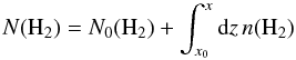 (6)where n(H2) is
the local density of H2 molecules and
N0(H2) is the quantity of H2 molecules
in the buffer that shields the medium from the external radiation field. We match
N0(H2) ≃ 1020 cm-2 to
Av0 = 0.1 by assuming this buffer is mainly
molecular. Similarly, we define N0(CO) for the CO
self-shielding but use N0(CO) = 0 because
Av0 = 0.1 is usually well below the
extinction at which CO is self-shielded in standard models of PDR.
(6)where n(H2) is
the local density of H2 molecules and
N0(H2) is the quantity of H2 molecules
in the buffer that shields the medium from the external radiation field. We match
N0(H2) ≃ 1020 cm-2 to
Av0 = 0.1 by assuming this buffer is mainly
molecular. Similarly, we define N0(CO) for the CO
self-shielding but use N0(CO) = 0 because
Av0 = 0.1 is usually well below the
extinction at which CO is self-shielded in standard models of PDR.
With this irradiation model, we integrated the chemical and thermal evolution of a fluid parcel with fixed density moving away from the radiation source at a constant velocity vPDR where the subscript PDR refers to the PDR. The resulting spatial profile (the trace of the thermal and chemical composition history of this fluid parcel along its path) corresponds to a steady PDR front moving towards the irradiation source at speed vPDR. For very low velocities we recover a steady PDR front that compares quite satisfactorily to the Meudon PDR code (Le Petit et al. 2006) for G0 = 1. In the frame of this comparison we switched off grains and polycyclic aromatic hydrocarbons (PAHs) reactions to remain closer to the Meudon PDR code setup. The PDR structure is insensitive to the choice of Lee et al. (1996) or Draine & Bertoldi (1996) for H2 photo-dissociation. This is because the rates differ only in regions where the absolute value of the rates are low, hence unimportant. For the same reason, we expect that our results only weakly depend on the exact value of the above mentioned Doppler parameter bD. Black & van Dishoeck (1987) also showed that this parameter is not crucial in PDRs.
Compared to Flower & Pineau des Forêts (2003), we refreshed the collision rates of OI by H atoms with the rates computed by Abrahamsson et al. (2007). These rates enter the computation of the atomic cooling due to O atoms. Atomic and molecular cooling are otherwise identical to those employed in Flower & Pineau des Forêts (2003). For instance, we used the molecular cooling rates tabulated in Neufeld & Kaufman (1993) for the cooling by CO and H2O.
Values for the main physical parameters in our models.
2.2. H2-excitation
We followed the time-dependent excitation of H2 along the shock structure as detailed in Flower & Pineau des Forêts (2003). Here, we include the treatment of the H2 population for the 149 lowest energy levels. We checked that this allows us to compute the H2 cooling accurately for shock velocities up to at least 40 km s-1 for the range of densities we consider in this work (see also Flower & Pineau des Forêts 2003).
We also used the knowledge of the population of the eight lowest H2 rotational levels to compute the rate of the reaction C+ + H2 more accurately. To compute the rate state by state, we used the information in Gerlich et al. (1987) (as in Agúndez et al. 2010, line 2 of Table 1) for H2 levels with J = 0...7 and v = 0 and the information in Hierl et al. (1997) (as in Agúndez et al. (2010), line 3 of Table 1) for the other levels.
2.3. Grains
As in Flower & Pineau des Forêts (2003), we treated adsorption, collisional sputtering, and collisional desorption of molecules from and onto grains. However, unlike these authors, we assumed pre-shock conditions without ice mantles. We accounted for the charge of grains by including all charge exchanges involving grains and electron detachment by cosmic-ray-induced secondary photons. The heating through the photo-electric effect was included, but we discarded the detachment of electrons that is caused by the radiation field in the chemical network.
3. Grid of models
3.1. Numerical protocol
For each value of our parameters described in the next section, we integrated the steady-state equations of multi-fluid MHD shocks (Flower et al. 1985; Heck et al. 1990) from entrance conditions at thermal and chemical equilibrium (see details of the pre-shock chemical conditions below). As stated above, we accounted for the changes in the properties of the irradiation field caused by the increasing absorption as we penetrated deeper into the shock structure. The computation was stopped when the temperature decreased to 20% above the temperature of the pre-shock.
3.2. Choice of parameters
We tuned most of our parameters to the typical conditions encountered in the dilute interstellar gas in our galaxy. We list the main physical parameters of our model in Table 1.
We indirectly specified the strength of the magnetic field transverse to the shock speed
by using the nondimensional parameter 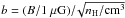 , which Crutcher et al. (2010) observed to take values from b = 0.1 to
b = 1 for our range of densities. We refer to these values below by
highly magnetised shocks for b = 1 and weakly magnetised shocks for
b = 0.1.
, which Crutcher et al. (2010) observed to take values from b = 0.1 to
b = 1 for our range of densities. We refer to these values below by
highly magnetised shocks for b = 1 and weakly magnetised shocks for
b = 0.1.
For both of these assumptions on the magnetic field, we built three grids of models, one
for each pre-shock density between
nH = 102 cm-3,
nH = 103 cm-3, and
nH = 104 cm-3. In the following, we
will use the term low velocity for shocks below 20 km s-1,
moderate velocity for shocks exceeding 20 km s-1, and
high velocity for shocks at and higher than 40 km s-1. Each
grid spans a range of velocities from 3 to 40 km s-1 with steps of
0.5 km s-1 for an integration time of about six hours per grid on a typical
workstation. We chose our lowest velocity of 3 km s-1 above the Alfvén speed in
the neutral gas for b = 1
 (7)where the mean mass per H nucleus is
μH = ρ/nH = 1.4
a.m.u. We chose the upper bound of 40 km s-1 because of the limitations of our
shock models1.
(7)where the mean mass per H nucleus is
μH = ρ/nH = 1.4
a.m.u. We chose the upper bound of 40 km s-1 because of the limitations of our
shock models1.
Elemental composition of the pre-shock gas (as in Godard et al. 2009).
At each fixed pre-shock density, we first evolved the gas chemically and thermally during 107 years, which brings the gas close to thermal and chemical equilibrium. We started with the same elemental abundances as in Godard et al. (2009), which are summarised in Table 2. The gas phase abundance in the pre-shock is set to a tenth of the Si locked in the grains cores, consistent with observations (Jenkins 2009). We also included PAHs with a fraction n(PAH)/nH = 10-6 of the representative species C54H18. Without irradiation (G0 = 0), PAHs influence the ionisation degree of the gas and the charge-ion coupling. However, with mild irradiation (at G0 = 1) the C+ ions dominate the charge fluid and the role of PAHs is negligible. With our current irradiation parameters (G0, extinction and H2 buffer), the atomic hydrogen fraction is n(H)/nH = 7.9(− 2), 1.3(–2) and 2.0(–3) in the preshock gas with respective densities nH = 102 cm-3, 103 cm-3 and 104 cm-3. We then used the resulting state as our pre-shock conditions to run the shock model for each velocity in turn.
3.3. C- and J-type shocks
Steady-state magnetised shocks in the interstellar medium are of two kinds: J-type shocks
in which the kinetic energy is dissipated viscously in a very sharp velocity jump
(hence “J”) followed by a thermal and chemical relaxation layer, and C-type
shocks in which kinetic energy is continuously (hence “C”) degraded into
heat and photons via ion-neutral friction and cooling. Mullan (1971) was first to discover that strong magnetic fields can transfer
kinetic energy to thermal energy in a continuous manner and coined the term C shock. Draine (1980), Draine
et al. (1983), and Roberge & Draine
(1990) then described the multifluid nature of these shocks. C shocks occur as
long as the shock velocity remains below the propagation speed of the magnetic precursor.
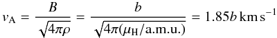
This critical velocity above which a C shock cannot exist is the magnetosonic velocity
 (8)where
  is the Alfvén speed in the charged
fluid and cs is the speed of sound. The Alfvén speed
in the charges depends both on the magnetic field and on the inertia in the charged fluid.
Thanks to the irradiation field, the gas is well ionised and provides ample free electrons
to stick onto the grains. As a result, most grains are charged negatively in our models
and hence they dominate the inertia in the charged fluid. Moreover, Guillet et al. (2007) showed that even the neutral grains spend an
extensive fraction of their time attached to the magnetic field and should also be
included in the charged fluid inertia. We hence included all PAH and grains in the
computation of the magnetosonic speed. As a result, the Alfvén speed in the charged fluid
vAc is higher than vA by a
factor
is the Alfvén speed in the charged
fluid and cs is the speed of sound. The Alfvén speed
in the charges depends both on the magnetic field and on the inertia in the charged fluid.
Thanks to the irradiation field, the gas is well ionised and provides ample free electrons
to stick onto the grains. As a result, most grains are charged negatively in our models
and hence they dominate the inertia in the charged fluid. Moreover, Guillet et al. (2007) showed that even the neutral grains spend an
extensive fraction of their time attached to the magnetic field and should also be
included in the charged fluid inertia. We hence included all PAH and grains in the
computation of the magnetosonic speed. As a result, the Alfvén speed in the charged fluid
vAc is higher than vA by a
factor  , where
ρ/ρd ~ 180 is the gas-to-dust mass
ratio. The actual number in our simulations is
vm = 21.2 km s-1, 21.7 km s-1, and
22.9 km s-1 for
nH = 102 cm-3,
103 cm-3, and 104 cm-3 for
b = 1 and about ten times lower values for b = 0.1.
, where
ρ/ρd ~ 180 is the gas-to-dust mass
ratio. The actual number in our simulations is
vm = 21.2 km s-1, 21.7 km s-1, and
22.9 km s-1 for
nH = 102 cm-3,
103 cm-3, and 104 cm-3 for
b = 1 and about ten times lower values for b = 0.1.
Shocks with speeds greater than vm will always be J shocks. For instance, all shocks in our b = 0.1 grid are J shocks. However, time-dependent shocks with velocities lower than vm could be C shocks, J shocks, or even a combination of the two (see Chièze et al. 1998; Lesaffre et al. 2004a,b). Indeed, (i) the transverse magnetic field could be lower for various orientations of the field (see Wardle 1998 for oblique C shocks); (ii) or the C shock could be at an earlier development of its structure where it still has a J shock component (Chièze et al. 1998; Lesaffre et al. 2004a); (iii) or the final fate of the shock could be a steady-state CJ shock, depending on the history of the shock (Lesaffre et al. 2004a,b). As a result, we built our grids of models with C shocks for shock velocities up to vm and used J shocks for higher shock velocities. In the following, we explore the properties of the resulting shocks.
3.4. Weakly magnetised shocks (b = 0.1)
For high compression ratios (i.e. Mach numbers much greater than 1), the maximum
temperature in a J shock (obtained just behind the leading adiabatic shock front) is
 (9)where μ is the mean
molecular weight of the gas, kB is the Boltzman constant, and
u is the shock velocity in the shock frame. The shock velocity is very
close to the velocity difference between upstream and downstream gas for high Alfvénic
Mach number. In particular, this relation shows that the peak temperature in a shock is
proportional to the square of the shock velocity.
(9)where μ is the mean
molecular weight of the gas, kB is the Boltzman constant, and
u is the shock velocity in the shock frame. The shock velocity is very
close to the velocity difference between upstream and downstream gas for high Alfvénic
Mach number. In particular, this relation shows that the peak temperature in a shock is
proportional to the square of the shock velocity.
For such dilute molecular gas, only the lowest energy levels of H2 are
populated and the appropriate value for γ is γ = 5/3.
With μ = 2.33 a.m.u. (which corresponds to the above
μH = 1.4 in our almost fully molecular conditions) relation
(9)becomes  (10)Figure 1a displays this theoretical value and the actual maximum temperature reached in
our models for each velocity tested in our grid at
nH = 102 cm-3. Both values remain
close to one another. At high temperature (high velocity), the maximum temperature is
closer to the value obtained in Eq. (9)with
γ = 7/5. This stems from the excitation of rotational levels of the
H2 molecules in the adiabatic front. We used a viscous length
λ = 1/σnH with a viscous
cross-section σ = 3 × 10-15 cm2 based on
H2-H2 collision data computed by Monchick & Schaefer (1980) for a velocity dispersion of 1 km s-1.
We checked that the viscous front between the peak temperature and the pre-shock is always
adiabatic. Its width of 1013 cm, visible in Fig. 1b, corresponds to the viscous length for
nH = 102 cm-3. This figure
surprisingly shows that higher velocity shocks return to pre-shock temperature on a
smaller distance than low-velocity shocks. However, the range of scales spans only one
order of magnitude from 2 × 1015 cm to 2 × 1014 cm with all
shocks with velocities higher than 20 km s-1 around the scale of
2 × 1014 cm. The range of flowing time through these shock structures also
spans about one order of magnitude, from 400 yr to 2000 yr. For higher densities, the
picture is much the same, and in particular time scales vary little within one category
(J-type or C-type) of shocks. However, shocks that strongly dissociate H2 (such
as dense shocks at moderate velocity) have a wide H2 reformation plateau where
H2 reformation provides the necessary heat to keep the gas warm (Flower et al. 2003).
(10)Figure 1a displays this theoretical value and the actual maximum temperature reached in
our models for each velocity tested in our grid at
nH = 102 cm-3. Both values remain
close to one another. At high temperature (high velocity), the maximum temperature is
closer to the value obtained in Eq. (9)with
γ = 7/5. This stems from the excitation of rotational levels of the
H2 molecules in the adiabatic front. We used a viscous length
λ = 1/σnH with a viscous
cross-section σ = 3 × 10-15 cm2 based on
H2-H2 collision data computed by Monchick & Schaefer (1980) for a velocity dispersion of 1 km s-1.
We checked that the viscous front between the peak temperature and the pre-shock is always
adiabatic. Its width of 1013 cm, visible in Fig. 1b, corresponds to the viscous length for
nH = 102 cm-3. This figure
surprisingly shows that higher velocity shocks return to pre-shock temperature on a
smaller distance than low-velocity shocks. However, the range of scales spans only one
order of magnitude from 2 × 1015 cm to 2 × 1014 cm with all
shocks with velocities higher than 20 km s-1 around the scale of
2 × 1014 cm. The range of flowing time through these shock structures also
spans about one order of magnitude, from 400 yr to 2000 yr. For higher densities, the
picture is much the same, and in particular time scales vary little within one category
(J-type or C-type) of shocks. However, shocks that strongly dissociate H2 (such
as dense shocks at moderate velocity) have a wide H2 reformation plateau where
H2 reformation provides the necessary heat to keep the gas warm (Flower et al. 2003).
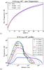 |
Fig. 1 a) Maximum temperature in the weakly magnetised shocks. b) Temperature profiles for some representative weakly magnetised shocks, the fluid flows from left to right with the pre-shock on the left and the post-shock on the right. Only J shocks are present for this low value of the magnetic field. nH = 102 cm-3. |
Figure 2a shows the total column density of H nuclei (NH) across each shock in the grid. Also displayed is the total H2 column density. The total NH column density is surprisingly constant around NH = 3–4 × 1018 cm-2 over the range of velocities in our grid except at the two ends. The increase of the compression factor at higher shock speed is compensated for by the shorter cooling length. This result is in contrast to the results obtained by Hollenbach & McKee (1989) in the velocity range 30 to 150 km s-1, where the cooling column density behind the shocks is seen to vary greatly. Shocks with velocities below about 7 km s-1 have a lower than average total column density, and shocks with velocities above 35 km s-1 dissociate H2, which decreases the amount of cooling and increases the total column density.
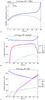 |
Fig. 2 For each shock velocity in our weakly magnetised shocks (b = 0.1), we plot a) the total H nuclei and H2 molecules column densities b) some neutrals of interest and c) some ions of interest; nH = 102 cm-3. |
Figures 2b and c show the total column densities across the shock for various neutrals and ions. We recall that the end of each shock is defined as the moment when the temperature decreases to 20% above the pre-shock temperature. Since the overall column density is a slowly varying function of the shock velocity (Fig. 2a), these plots also give a good estimate on how the average relative abundance of each of these species varies with respect to the shock velocity. One striking feature of these figures is the sharp rise of some molecular abundances at low velocity. We traced these apparent velocity thresholds to temperature barriers or endothermicities of key reactions that initiate the production of molecules. Equation (10)allows us to relate these critical temperatures to the key velocities in J shocks. We list in Table 3 the main bottleneck reactions that involve H2 and a single atom or monoatomic ion along with their characteristic temperatures and J shock velocities. At high velocities, the decrease in molecular content (around 35 km s-1) corresponds to the absence of H2 molecules due to dissociation in the shock front.
Figure 2c illustrates the variation of a few ions of
interest. The abundance of C+ is controlled mainly by photo-ionisation of C and
charge exchange with PAHs and H2. As the velocity increases, the post-shock
density increases with enhanced charge exchange, thus decreasing the C+
abundance. For very high velocities (above 35 km s-1) H2 starts to
be dissociated and C+ increases again. In a molecular medium, the abundance of
is controlled by the balance between
cosmic ray ionisation of H2 (followed by a hydrogen exchange with
H2) and recombination of . The charge balance links the ionisation
degree to the abundance of C+, thus the abundance of
is inversely proportional to C+
with an extra dependence on the square root of the temperature due to the temperature
sensitivity of the recombination rate.
In Fig. 3 we display the variation of the total emission of various lines of interest depending on the shock velocities. This can be of interest for observers who aim to characterise the velocities of observed shocks. Figure 3a shows some of the most observed atomic lines with the H2 0-0 S(1) line for comparison. The C+ ion emission decrease at moderate velocities is an abundance effect. Atomic O cooling is enhanced at moderate velocities because these shocks dissociate H2: this slows down the cooling and yields a temperature plateau where O is the dominant cooling agent. The stronger the shock, the longer it takes for H2 to reform, then the plateau widens and the O emission increases.
Figure 3b shows how the lowest energy lines of H2 change with the velocity of the shock. The relative strengths of these lines vary greatly between u = 3 km s-1 and u = 10 km s-1. For example, the ratio S(1)/S(3) decreases from more than a hundred at 3 km s-1 to about a fifth at 10 km s-1. Indeed, the shock peak temperature in this range of velocities spans the energies of the upper levels of these transitions (J = 7 corresponds to 3474 K, for instance, and see Fig. 1a for how the maximum temperature in the shock varies with shock velocity): the excitation diagram in the low levels of H2 is greatly affected in this range of temperatures. By contrast, the aspect of the excitation diagram does not change above 10 km s-1: the emissivities of these lines are unable to distinguish the shock velocity u for u > 10 km s-1. Indeed, above 10 km s-1 the temperature experienced in these shocks is much greater than the J = 7 energy. Observers should use lines with upper levels with higher J values (such as rovibrational lines) to probe the velocities of these shocks, or they should use diagnostics based on atomic lines.
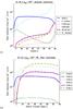 |
Fig. 3 a) Atomic and b) pure rotational H2 line emission for weakly magnetised shocks. nH = 102 cm-3. |
In Fig. 4 we examine that fraction of the kinetic
energy flux input 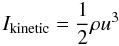 (11)into the shock that is radiated away by each
coolant. Individual coolings are integrated through the whole shock structure as follows:
(11)into the shock that is radiated away by each
coolant. Individual coolings are integrated through the whole shock structure as follows:
 (12)where Λ is the local rate of cooling and
x1 is the end point of the shock (i.e. where the temperature
decreases to 20% above the pre-shock temperature). We also display the magnetic energy
flux accross the shock,
(12)where Λ is the local rate of cooling and
x1 is the end point of the shock (i.e. where the temperature
decreases to 20% above the pre-shock temperature). We also display the magnetic energy
flux accross the shock,  (13)where ui is the
ion velocity and Be is the magnetic field at the end of the
shock. H2 cooling dominates almost everywhere except (i) at very low velocity,
where atomic O or C+ cooling takes over depending on the density; and (ii)
above the velocity for H2 dissociation (which is lower for higher densities),
where atomic O and H (Lyman-α) cooling take over. At density
nH = 104 cm-3, and below
20 km s-1, note that H2O cooling becomes important.
(13)where ui is the
ion velocity and Be is the magnetic field at the end of the
shock. H2 cooling dominates almost everywhere except (i) at very low velocity,
where atomic O or C+ cooling takes over depending on the density; and (ii)
above the velocity for H2 dissociation (which is lower for higher densities),
where atomic O and H (Lyman-α) cooling take over. At density
nH = 104 cm-3, and below
20 km s-1, note that H2O cooling becomes important.
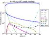 |
Fig. 4 Cooling integrated along the shock length, normalised by kinetic power
|

3.5. Strongly magnetised shocks (b = 1)
In a C shock, the kinetic energy is continuously transformed into thermal energy via
ion-neutral friction. As a result, the heating is spread out on a much more extended
region than for J shocks and the peak temperature is hence much lower as seen in
Fig. 5a. However, reactions between neutral and ion
species benefit from the ion-neutral drift, and the effective temperature that is used to
compute the reaction rate is higher (see Pineau des Forêts
et al. 1986). For instance, the effective temperature for reactions involving
C+ and H2 is
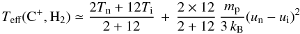 (14)where
(un − ui) is the local drift
velocity between the ions and the neutrals, mp is the proton
mass and Tn and Ti are
respectively the temperatures of the neutral and ionised gas. Figure 5a shows the maximum effective temperature of the reaction C+
+ H2, which incidentally is very close to the highest temperature that would be
obtained in the corresponding J shock.
(14)where
(un − ui) is the local drift
velocity between the ions and the neutrals, mp is the proton
mass and Tn and Ti are
respectively the temperatures of the neutral and ionised gas. Figure 5a shows the maximum effective temperature of the reaction C+
+ H2, which incidentally is very close to the highest temperature that would be
obtained in the corresponding J shock.
Compared to the temperature profile of a J shock, the temperature profile of a C shock is broad, with a lower temperature: see Fig. 5b. However, within each type of shock, the total size of the shock structure varies over less than an order of magnitude for the range of velocities we tested, as is apparent in Fig. 5b. This is even more striking for the flowing time scale across the shock structures which, for nH = 102 cm-3, varies only from 8000 to 6000 years for the C shocks and from 1500 to 1000 years for the J shocks. As mentioned above, this holds for higher densities as well.
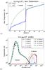 |
Fig. 5 a) Highest temperature in the highly magnetised shocks. b) Temperature profiles for some representative highly magnetised shocks; the fluid flows from left to right with the pre-shock on the left and the post-shock on the right; nH = 102 cm-3. |
Slightly above 20 km s-1, all shocks in our grids of models are J shocks, but the strength of the magnetic field varies from b = 0.1 in the previous subsection to b = 1 in this subsection. The higher magnetic field limits the compression in the shock and the collisional processes take longer to occur. In particular, the cooling length for the J shocks above 20 km s-1 is between 4 × 1015 cm and 7 × 1015 cm: much wider than for the corresponding weakly magnetised J shocks. The lower density but larger size of the shock impacts on the chemical composition and structure in subtle ways. A careful comparison of the right hand sides of Figs. 2 and 6 shows that the column density of H nuclei is higher in magnetised shocks and moderate variations in the chemical composition are noticeable.
Figure 6 shows the molecule production over the range of models in our grid at nH = 102 cm-3. The transition from C shocks (velocity lower than 21 km s-1) to J shocks (higher shock speed) is clear. The column densities of most species have a drop at 21 km s-1 that expresses a boosted molecular production in C shocks. Three effects are at play that favour molecule production in C shocks.
First, the ion-neutral drift helps to overcome reaction barriers of ion-neutral reactions (which impact C-bearing species, for example, whose bottleneck reaction is C++H2). Second, the resulting frictional heating keeps the temperature warm throughout the shock. By comparison, a J shock is very hot at the peak temperature immediately behind the viscous front, but quickly cools down in the trailing relaxation layer. Third, the steady frictional heating slows down cooling and compression in the relaxation layer, and the net result is an increased total NH column density in C shocks compared to J shocks (see the drop at 21 km s-1 in Fig. 6a). This is the main factor that impacts those molecular species whose production relies mainly on neutral-neutral reactions (such as O-bearing species). In particular, these species show a more gradual rise at low velocities, because of the slower rise of the maximum neutral temperature in C shocks.
We display the total integrated emission in various lines of interest in Figs. 7a and b: as for Fig. 3, these give clues on which observations constrain what shock velocity. In particular, the emissivities of H2 lines with low-J upper levels now vary from 3 to 20 km s-1, but are independent of velocity above 20 km s-1. The neutral temperature in C shocks rises more slowly than J shocks, as shown by the comparison between Figs. 1 and 5, but the maximum temperature in C shocks is more representative of the temperature in the whole mass of the shock and the column density in C shocks is higher. As a result, the left hand sides (between 3 and 20 km s-1) of Figs. 7a and b look like blow ups of Figs. 3a and b shifted to greater emissivities. However, C+ stands out even more for C shocks because its excitation benefits from the ion-neutral drift. The right-hand sides of Figs. 7a and b are similar to the corresponding weakly magnetised J shocks seen in Figs. 3a and b: the emissivities are only weakly affected by the density change caused by the magnetic field except for C+.
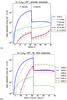 |
Fig. 7 a) Atomic and b) rotational H2 lines emission for highly magnetised shocks. nH = 102 cm-3. |
In Fig. 8 we examine, averaged over the whole shock structure as in Fig. 4, the fraction of the kinetic energy flux input into the shock that is radiated away by each coolant in the low-density case (nH = 102 cm-3). At very low velocity, C+ is the most efficient coolant (rather than O for weakly magnetised shocks), but H2 takes over for shock velocities shortly above 5 km s-1. Molecules such as CO, H2O, or OH carry less than a percent of this energy flux. The kinetic energy flux is mainly transferred into a magnetic energy flux (via field compression) for velocities below 10 km s-1 and is mainly radiated away above that velocity. At higher densities, the low-velocity coolant becomes O. It is also interesting to note that at nH = 104 cm-3 H2O becomes an important cooling agent for low velocities. Flower & Pineau des Forêts (2010) also quoted the fraction of energy radiated away in various cooling processes in their shock models. However, in the present work the irradiation field photo-dissociates CO and ionises C so that C+ cooling is more prominent and CO cooling is less important than in their work, but the results are otherwise similar. In particular, Flower & Pineau des Forêts (2010) also found that the magnetic energy flux stores 50% of the injected power at u = 10 km s-1.
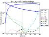 |
Fig. 8 Cooling normalised by kinetic power in highly magnetised shocks for a pre-shock density nH = 102 cm-3. The solid line with triangles shows the fraction of the power that is transferred into a flux of magnetic energy. |
4. Probability distribution functions of shocks
4.1. Method of fit
Numerical simulations of driven supersonic turbulence show that the medium experiences a whole range of shock speeds: Smith et al. (2000) showed that the probability distribution function (PDF) of the velocity jumps follows a decreasing power law with an exponential cut-off at a Mach number of a few. Pety & Falgarone (2000) carefully separated vortical from compressional contributions in the velocity field of a compressible simulation of decaying supersonic turbulence: they uncovered an exponential distribution for the convergence time scales −1/div(v) where v is the fluid velocity. Subsonic wind tunnel experiments displayed an exponential distribution of velocity increments (Mouri et al. 2008).
These results hint at a variety of possible PDF shapes for the statistics of shocks, all favourably weighted towards low-velocity shocks. Guillard et al. (2009) have modelled Spitzer H2 observations of SQ with only two discrete values of the shock velocities. Here, we aim at fitting a statistical distribution of shocks to a collection of observed quantities. Guided by the above remarks on turbulence, we fitted various shapes of shock PDFs: decaying exponentials, power-laws, Gaussians, and a piece-wise exponential fit.
Template PDFs adjusted to the observed data (normalisation constants are discarded as irrelevant, see text).
We considered among j = 1...M
observable quantities an observable
Xj(u) associated to a
steady shock of velocity u (expressed in km s-1). We denote
with
f(u, {pi} i = 1...N)
the probability density parametrised by the set of parameters
{pi} i = 1...N.
Of course, the fitting is meaningful only as long as the number of observed quantities
M is sufficiently greater than the number of fitted parameters
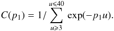
N. For example, an exponential PDF reads
 (15)with the normalisation constant
 (16)We then computed observable quantities
averaged over the PDF of shocks as
(16)We then computed observable quantities
averaged over the PDF of shocks as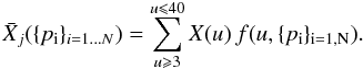 (17)To facilitate the fitting process, we
normalised the above values to the sum of the observable quantities:
(17)To facilitate the fitting process, we
normalised the above values to the sum of the observable quantities:
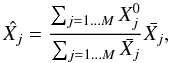 (18)where
  are the actual observed values. Note that
this normalisation renders the normalisation constant of each PDF irrelevant, but it
decreases the number of degrees of freedom by one unit
Mfree = M − N − 1. We
finally find the optimal set of parameters
are the actual observed values. Note that
this normalisation renders the normalisation constant of each PDF irrelevant, but it
decreases the number of degrees of freedom by one unit
Mfree = M − N − 1. We
finally find the optimal set of parameters  which minimises the quantity
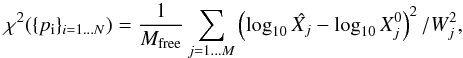 where
Wj is the uncertainty on the observed
value
where
Wj is the uncertainty on the observed
value  . We also retrieved estimates
{Ei} i = 1...N
of the errors on the parameters by computing the diagonal elements of the covariance
matrix of
. We also retrieved estimates
{Ei} i = 1...N
of the errors on the parameters by computing the diagonal elements of the covariance
matrix of  on the optimal set.
Table 4 summarises the various PDFs and their parametrisation. The exponential and power-law PDFs are motivated by the above mentioned work on the statistical distribution of shocks in numerical and laboratory experiments. The piece-wise exponential PDF is built in intervals designed such that the observable quantities vary significantly (cf. Figs. 3 and 7). Otherwise, the parameters would be degenerate. We used as parameters the PDF value at the transition between these intervals. Thus, these parameters’ optimal values and corresponding error bars directly probe the PDF and its uncertainty at these chosen locations. Finally, we used a single or a double Gaussian PDF to mimic the fit of one shock or two independent shocks: this allows one to connect with the work of Guillard et al. (2009).
In addition, we note that the choice of the boundaries (upper and lower velocities) for the range of our grid of models does not significantly affect our results. This is because the shock emission is very low at low velocity and high-velocity shocks are very rare in the solutions we obtain. Finally, grids of models with velocity spacings of 1 km s-1 and 0.5 km s-1 gave similar results, which validates the resolution we chose.
4.2. Applications
4.2.1. Stephan’s Quintet galaxy collision
In this section we use our model results to fit H2 line emission from the galaxy-wide shock in SQ. This shock structure, first identified in radio continuum observations and X-ray images, was discovered to be a luminous H2 source with Spitzer (Appleton et al. 2006; Cluver et al. 2010). It is associated with the entry of a galaxy into a group of interacting galaxies with a relative velocity ~1000 km s-1. The luminosity of the molecular gas in H2 rotational lines is observed to be higher than that of the plasma in X-rays. Guillard et al. (2009) presented a first interpretation where the H2 emission is powered by dissipation of turbulence driven by the large-scale collision. CO observations have since shown that the kinetic energy of the molecular gas is larger than the thermal energy of the hot (X-ray emitting) plasma. It is the main energy reservoir available to power the H2 line emission (Guillard et al. 2012). Guillard et al. (2009) showed that the H2 excitation is well fitted by a combination of two MHD shocks with velocities of 5 and 20 km s-1 in dense gas (nH ~ 103 to 104 cm-3), using the shock models of Flower & Pineau des Forêts (2003), which do not take into account UV radiation. Our grid of models allows us to test an alternative interpretation where the H2 emission is accounted for with MHD shocks in lower density UV irradiated gas. In doing so, we quantify a solution where the physical state of the H2 gas in SQ is akin to that of the cold neutral medium in the Galaxy. Evidence that the gas is magnetised comes from radio continuum observations. The synchrotron brightness of the shock yields a magnetic field value B ~ 10 μG, assuming equipartition of magnetic and cosmic-ray energy (Xu et al. 2003). This value is comparable to the field strength reported by Crutcher et al. (2010) for the Galactic diffuse ISM. The mean UV radiation field in the SQ shock estimated to be G0 = 1.4 (Guillard et al. 2010), is also close to the reference value for the ISM in the solar neighbourhood.
The wide extension (30 kpc) of the SQ shock suggests that in the relaxation layer that follows the main high-velocity (~600 km s-1) shock, a large number of substructures are formed that then collide and yield a range of subshocks with much lower velocities (see Guillard et al. 2009). Simulations of large-scale shocks subject to thermal instability indeed show that turbulence is sustained in the trailing relaxation layer (Koyama & Inutsuka 2002; and later Audit & Hennebelle 2005, 2010; Hennebelle & Audit 2007). This connects with the theoretical work on turbulence mentioned above, and justifies our investigation with continuous PDFs of shock velocities. The observable targets that we aim to reproduce are the emission values for the six H2 lines 0-0 S(0) to S(5) in Table 1 of Cluver et al. (2010), which are integrated over the main shock structure.
Table 5 shows the best χ2 obtained in all our attempts to fit the data. Two solutions stand out with χ2 values reasonably close to one, the piece-wise exponential and the two Gaussians at b = 1 and nH = 102 cm-3 (their χ2 values are emphasised in bold faces in Table 5). Figure 9 illustrates the quality of the fit on the observed H2-lines. Our models reproduce every H2-line quite accurately except for 0-0 S(4) 2. For comparison, when we use the same technique and same grid of models as Guillard et al. (2009) (i.e.: models without irradiation at nH = 104 cm-3), we find that the best fit is obtained for two shocks of velocity 5 and 22 km s-1 in proportion 1:0.008 with a reduced χ2 = 78 (compared to χ2 = 15.8 for velocities 3.7 and 21 km s-1 in proportion 1:0.0002 in our two-Gaussians high-density case). The coincidence of the best parameters with our two-Gaussian solution is surprising, but the improvement on the χ2 in the present work is also striking. Irradiation does indeed improve the comparison with the observations. Our work also shows that low-density solutions are even more viable than the previously found high-density solutions.
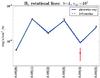 |
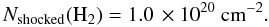
Fig. 9 Observed fluxes of the H2 lines in the SQ (red dots with error bars: Cluver et al. 2010, see also Table 6) with the results of our best two models. Most error bars are so small they are barely visible. |
All best PDF shapes we found (including those with a high χ2) are statistically biased towards low-velocity shocks. Figure 10 displays the two best-fit PDF solutions. The error bars (grey regions in these figures) are determined as follows: we varied the parameters of the PDFs at the extreme of their 3-σ range of uncertainty and assumed the lowest and highest values predicted when using these extreme PDFs. The piece-wise exponential adjustment shows a dip at 10 km s-1, which indicates a bimodal distribution of shocks consistent with the two-Gaussian fit (which is bimodal in essence). Perturbation tests of this fit show that the PDF level at 10 km s-1 depends mainly on the ratio S(0)/S(1), with a deeper dip for higher values of this ratio. On the other hand, the currently observed data do not distinguish whether the distribution of moderate velocity shocks is widespread or clearly centred on a distinct velocity. Indeed, as seen in Fig. 7b, above 20 km s-1 the emission properties of the observed H2 lines do not change with velocity, hence these lines cannot probe the shape of the PDF in this range of velocities. Ro-vibrational lines should be used to probe the shocks at these velocities. All piecewise-exponential solutions (including those with a higher χ2 at higher densities) are similarly consistent with bimodal distributions. This is not expected from the statistics of shock velocities in numerical simulations of turbulence. It may be a result of the intrinsic multiphase nature of the interstellar medium, where the moderate velocity shocks would be interpreted as collisions between molecular clouds, and low-velocity shocks would be the signature of turbulence dissipation within these clouds.
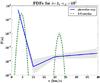 |
Fig. 10 Shape of our best two PDFs fit to the SQ data. Grey areas represent uncertainties due to the propagation of observational errors (see details in text). |
For each of the best PDF found, we can predict the value
 of other quantities of interest. We provide in Table 6 the total column densities for some molecules and the expected emission of
some atomic lines in our best two solutions. These total column densities are integrated
from the pre-shock to the point where the temperature decreases to 20% above the
pre-shock temperature. In particular, we provide a measure of the total H2
column density: the piece-wise exponential model yields
of other quantities of interest. We provide in Table 6 the total column densities for some molecules and the expected emission of
some atomic lines in our best two solutions. These total column densities are integrated
from the pre-shock to the point where the temperature decreases to 20% above the
pre-shock temperature. In particular, we provide a measure of the total H2
column density: the piece-wise exponential model yields
 and the two-Gaussian model yields
 Recent measurements from CO spectroscopy
(Guillard et al. 2012) allow one to estimate
the total H2 column density in the SQ large-scale shock structure as
Recent measurements from CO spectroscopy
(Guillard et al. 2012) allow one to estimate
the total H2 column density in the SQ large-scale shock structure as
 (assuming a Galactic value for the CO
emission to H2 column conversion factor). This puts the fraction of shocked
gas in this line of sight between 32% and 12%, depending on which model we adopt, which
confirms the results of Guillard et al. (2010)
that quite substantial amounts of gas are shock-heated. Indeed, quite a few of our best
solutions predict
Nshocked(H2) > 1021 cm-2
and are therefore probably ruled out (only the viable solutions are underlined in Table
5).
(assuming a Galactic value for the CO
emission to H2 column conversion factor). This puts the fraction of shocked
gas in this line of sight between 32% and 12%, depending on which model we adopt, which
confirms the results of Guillard et al. (2010)
that quite substantial amounts of gas are shock-heated. Indeed, quite a few of our best
solutions predict
Nshocked(H2) > 1021 cm-2
and are therefore probably ruled out (only the viable solutions are underlined in Table
5).
Since the shocks account for a significant fraction of the gas mass, any chemical enhancement in the shocks may have a significant contribution to molecular abundances. Table 6 also gives estimates of the chemical yields in these shocks. For example, the H2O abundance is about 10-6, significantly greater than that observed in the diffuse ISM in the Milky-Way (Wyrowski et al. 2010). These abundances could be even higher if the medium is clumped (and therefore shielded), and Herschel may provide a good opportunity to test this. For standard irradiation C+ is the dominant carbon gas species, which is also a result that will depend on shielding.
Summary of the best χ2 values obtained in all our attempts to fit the SQ data.
Results of our best two fits to the observed spectral line energy distribution in SQ and their respective predictions.
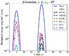 |
Fig. 11 Distribution of the energy dissipated via several cooling agents for the two-Gaussian best-fit model. |
The importance of these species (in addition to H2) as cooling agents of the interstellar turbulence directly depends on their abundance. Herschel observations could thus provide additional constraints to achieve a precise modelling of the physical and chemical state of the gas. We provide estimates of the total integrated flux in the molecular cooling agents in Table 6: H2 itself is responsible for more than 94% of the cooling in both our best-fit models. However, its emission is distributed over many different lines, the strongest of which, H2-S(1), contributes by a few percent of the total. For low-velocity C-type shocks the pure rotational lines add up to almost the entire H2 cooling. In contrast, moderate velocity J-type shocks experience much higher temperatures, and the energy in these shocks is radiated away through higher H2-levels. If our models with a contribution from moderate velocity J shocks hold, much more energy should be emitted from higher excitation levels of the H2 molecule than is observed from pure rotational lines. Finally, other molecular coolants contribute at most a few percent of the H2-S(1) luminosity.
The emission of the C+ line at 158 μm is quite strong in our best two models (about half as strong as the H2-S(1) line), and so is the OI emission to a lesser extent. Assuming all carbon is in the form of C+ in the unshocked fraction of the total line of sight column density Ntotal(H2), we predict that the C+ line should shine about as much as the H2-S(1) line, with a significant contribution from shocks (66% and 52% in the two models). Interestingly, this was also suggested in an interpretation of AKARI observations by Suzuki et al. (2011). In contrast, the model proposed by Guillard et al. (2009) without UV irradiation has no CII emission. This means that C+ can indeed be a good signature for the dissipation of kinetic and magnetic energy in weakly shielded gas (as previously found by Falgarone et al. 2007). We also note that our viable models at higher densities predict even stronger emission in C+ by up to a factor of three. As such, C+ emission measurements will help to probe both the density and shielding of the gas. In contrast to C+, the measured emission of the Si+ line at 34.8 μm is much higher than the predicted emission from our shock models. It is probably dominated by the contribution from the hot ionised medium, as already suggested by Cluver et al. (2010).
Figure 11 displays the distribution of energy radiated away for several cooling agents in the best-fit two-Gaussian solution. A significant fraction of energy is dissipated in low-velocity shocks, but more energy is radiated within moderate velocity shocks. Indeed, the dissipated power behaves as the cube of the velocity, which slightly more than compensates for the higher number of low-velocity shocks. The figure clearly demonstrates that H2 is by far the main cooling agent. It also shows that the emission from atomic cooling agents comes mainly from low-velocity shocks, whereas the molecular emission is dominated by moderate velocity shocks. Similarly, we have checked that the emission from low J H2-lines probe low-velocity shocks, whereas higher J lines probe higher velocity shocks, which seems rather natural.
4.2.2. Chamaeleon
Nehmé et al. (2008) successfully interpreted observational results of a line of sight sampling diffuse molecular gas in front of the star HD 102065 in Chamaeleon. Their PDR model with G0 = 0.4, nH = 80 cm-3 and Av = 0.67 accurately reproduced as many as seven independent observational quantities. However, the authors were unable to account for the column densities of rotationaly excited states of H2 and failed to reproduce the observed abundance of CH+. Here, we assumed that both a PDR and a statistical distribution of shocks contribute to this line of sight. Hence we attempted to fit as many as 11 observational measurements available for this line of sight with a linear combination of our shock models and a PDR model.
The PDR model was computed with our shock code in a PDR mode, see Sect. 2.1. In principle, we should fit all irradiation parameters of the PDR alongside the grid of shocks. But this would entail recomputing the whole grid of shocks each time we probe new irradiation parameters and would lead to prohibitive computational times. Hence we fixed the irradiation conditions and the PDR model therefore introduces only one additional parameter in the fit: its weight in the line of sight compared to the shock models. We used G0 = 4 and Av = 0.335 as entrance conditions for both the PDR and the shocks and computed a new grid of shock models from 3 to 40 km s-1 with nH = 80 cm-3 and an ortho/para ratio of 0.7 as observed.
We thus obtained reasonable χ2 values with a best value of 11 for both the two-Gaussian and the piecewise-exponential. The error mainly comes from overestimating the column density in J = 5, but the molecular chemistry of the line of sight is reproduced quite accurately (see Table 7).
The two best-fitting PDFs compare qualitatively well to the solutions we found for SQ, except that the low-velocity part of the two-Gaussian is more tightly peaked on low velocities (the moderate-velocity component accounts for 3% of the total probability), and the piecewise-exponential dip at 10 km s-1 is less pronounced. The two PDF shapes are hence slightly less consistent than for SQ, and continuous solutions are not ruled out (the exponential and power-law solutions yield χ2 values of about 20 and 15). However, for the Chamaeleon, the physical extent of the measured beam is much smaller than for SQ. In particular, the total number of shocks involved is presumably much smaller and discrete number effects might appear in the distribution.
Results and predictions of the fit of piecewise-exponential to the Chamaeleon data (Gry et al. 2002; Nehmé et al. 2008).
Our best two models predict similar values for most of the observables listed in Table 7. We now have two contributions from the PDR and the shocks, and for each quantity listed in Table 7 we quote in brackets which fraction comes from the shocks. The weight of the PDR model in both best solutions is slightly different, which yields a mass fraction of shocked matter on the line of sight of 4% in the piecewise-exponential model and 19% in the two-Gaussian model. The contribution from shocks is hence small but not insignificant. However, molecules other than H2 are all formed in the shocks and not in the PDR, with 98% of the CO coming from the shocks, for example. In our two best models, shocks with velocity above 15 km s-1 account for the formation of almost all molecules. This is because the chemical barriers are overcome thanks to the thermal energy released in shocks and thanks to the ions-neutrals drift, as mentioned in Sects. 3.4 and 3.5.
CH+ needs a mechanical energy injection to raise the effective temperature
for its formation, which is why pure PDR models failed to account for its abundance.
Indeed, CH+ forces a component into the model that is too hot, which then
overproduces the J = 5 H2-level. A possible solution would
be that the irradiation in the far-UV is enhanced in the Chamaeleon compared to the
Draine ISRF: this would make more CH+ from
 and
and
 photo-dissociation (Falgarone et al. 2010) while requiring a lower
temperature more compatible with the observed J = 5 H2-level
column density. Indeed, UV spectra in Boulanger et al.
(1994) suggested that the enhanced far-UV field could be accounted for by a
flatter extinction curve in the far-UV for this very line of sight.
photo-dissociation (Falgarone et al. 2010) while requiring a lower
temperature more compatible with the observed J = 5 H2-level
column density. Indeed, UV spectra in Boulanger et al.
(1994) suggested that the enhanced far-UV field could be accounted for by a
flatter extinction curve in the far-UV for this very line of sight.
As in SQ, H2 is by far the main cooling agent (it radiates more than 92% of the total cooling in the two best-fit models), but CII (and OI to a lesser extent) has an emission comparable to the H2-S(1) line. Even though it is dominated by the emission from the PDR, the shock contribution to CII emission is still significant (from 18% to 31% according to the two best models). Interestingly, we predict that OH will shine about as much as CII, and as for the SQ solution, the OH emission is almost completely dominated by the contribution from shocks at moderate velocity. OH observations would hence provide a good test of the possible existence of a moderate-velocity shock component in the Chamaeleon.
5. Summary, conclusions, discussion, and prospects
We provide a grid of shock models3 in UV-heated gas that may be used to interpret observations of the Milky Way diffuse ISM and integrated properties of galaxies in general. We examined magnetised shocks in media with densities from nH = 102 to 104 cm-3, with standard ISM irradiation conditions and at low- to moderate velocities (from 3 to 40 km s-1). When the velocity of these shocks was below the critical velocity for the existence of pure C-type shocks, we computed C-type shocks, otherwise, we computed J-type shocks. The models include the effects of the ambient UV irradiation field on the pre-shock chemistry and thereby on the relative importance of cooling lines in the shock. For instance, C+ can provide significant line cooling in shocks propagating in the UV-irradiated gas, where it is the dominant carbon species.
We illustrated how the model results may be used to interpret data on one galactic line of sight through the diffuse ISM (Chamaeleon) and one extra-galactic object (the SQ shock). We fitted the observables with a continuous combination of shock models as a phenomenological description of the complex statistical properties of the turbulence dissipation. The model provides quite a good match to the data for bimodal distributions of shock velocities. This does not agree with predictions from numerical simulations of Smith et al. (2000), who found a power-law distribution with an exponential cut-off. More work is needed to understand the reasons behind this apparent discrepancy. Interestingly, the low- and moderate velocity components of our best-fit PDF operate in very different regimes of energy dissipation. Indeed, in our best-fit models to the observations, the low-velocity shocks are of C-type and dissipate energy via ion-neutral drift, whereas the higher velocity shocks are of J-type and undergo viscous dissipation.
In both our interpretations of SQ and the Chamaeleon, a significant fraction of the molecular gas is shock-heated, and the chemistry in this shock-heated gas has a dominant contribution to key molecules such as CO, H2O, OH or CH+, which are commonly used as diagnostics. This shock-heated contribution might be greater than the contribution of CO computed in simulations by Glover & Mac Low (2011), where the resolution in the shocks is too low to trigger the shock chemistry: an insufficiently low resolution smears out the temperature to such an extent that shocks become nearly isothermal with a temperature too low for molecule formation. Furthermore, although low-velocity shocks are less efficient than moderate-velocity shocks, they are more numerous, and depending on the statistical distribution of shocks they could potentially account for a higher fraction of the excitation and formation of molecules.
Shocks in the line of sight also have important consequences on the emission of C+. Indeed, C+ is usually considered as a good tracer of the ambient UV radiation field, and indeed, the mere presence of the C+ ion is conditioned to its photo-ionisation. But we showed here that the emission of C+ in both SQ and Chamaeleon has a significant contribution from gas heated by the dissipation of kinetic energy rather than by UV photons, as is the case in PDRs.
The SQ H2 excitation diagram was fitted with low- and moderate-velocity C shocks in dense UV-shielded gas (nH = 104 cm-3, G0 = 0) in previous studies (Guillard et al. 2009). We showed that a better fit can be obtained with diffuse irradiated gas (nH = 102 cm-3, G0 = 1) including J-type shocks. If this second solution is the appropriate one, C+ is a significant coolant of the shocked medium. This prediction can be tested with the Herschel observatory. The presence of the high-velocity J shocks can also be tested through the emission in H2-lines coming from rovibrational levels.
OI, H2O, OH, and CO provide additional diagnostic lines that could help in constraining the physical state of the gas and the dissipation processes. OI is seen to be significant at higher densities, whereas C+ is significant for lower densities. Molecules such as H2O, OH, and CO evacuate less than one percent of the total kinetic power except at high densities where H2O in C shocks can contribute as much as 10%.
The remainder of the incoming power in our shocks is converted into a flux of magnetic energy. The differences in total pressure (magnetic plus thermal) between the shocked regions and the regions that have not been shocked will initiate new motions: the energy stored in the post-shock compression will eventually give rise to expansion motions, with an effective transfer back to kinetic energy. Thus, shocks are actors that contribute to the equipartition between various forms of energy, thanks to a continuous recycling of the gas throughout successive shock structures.
The main caveat of our study is that we assumed the relaxation of the post-shock pressure takes place instantaneously: our model accounts for the pre-shock gas and the shocked gas, but does not incorporate the expansion of the gas after the shock. We will attempt to model this phase in future studies. Another caveat of our study lies in the implicit assumption that all shocks are steady. Indeed, some shock velocities are prone to instabilities and even quasi-steady models are invalid in this case (see Lesaffre et al. 2004b, for example). Less important caveats are the shock orientation, its curvature, the neglect of intermediate ages of shocks (for ages younger than about 104 yr, we should consider CJ-type shocks or non-steady shocks). We believe that these minor caveats are balanced because we fitted a statistical collection of shock velocities. Finally we did not treat UV pumping in the H2-population, but Monteiro et al. (1988) showed that this begins to make a difference only for H2 levels above J = 5 and for G0 ≫ 1.
Our PDF fitting technique might prove useful to account for single shocks with more complicated geometries. For example, a single bow-shock effectively encompasses a continuous collection of velocities depending on the angle at which each fluid parcel of pre-shock gas impinges on the bow-shock. In this framework, the shape of the lines is directly related to the dynamics inside the shock, and not simply due to the relative motions between each shocks as in the statistical distribution of shocks we inferred in SQ. In these cases, it will therefore be interesting to predict and use the line shapes as additional observational constraints on the shock physics.
Finally, as we already mentioned, the dissipation of turbulent motions does not occur in shocks only. It will be interesting in future work to assess on the one hand the fraction of the energy dissipation that takes place in vortices, current sheets, or shocks, for example. On the other hand, it will be worth comparing vortex models as in Godard et al. (2009) to our own shock models to check whether we can observationally distinguish the respective signatures of shocks and vortices.
Indeed, the code does not treat doubly ionised species and radiative emission from the post-shock itself, which might affect pre-shock conditions at high densities (see Flower & Pineau des Forêts 2010).
This line lies at the position of the 7.7 μm PAH emission feature, which makes it difficult to measure accurately.
The output data at our models are archived on http://cemag.ens.fr and at the CDS.
Acknowledgments
P.L., E.F., and B.G. acknowledge support from SCHISM A.N.R.. We thank Maryonne Gerin and Antoine Gusdorf for comments on the manuscript. We thank the anonymous referee for his/her comments, which improved the readability of the paper.
References
- Abrahamsson, E., Krems, R. V., & Dalgarno, A. 2007, ApJ, 654, 1171 [NASA ADS] [CrossRef] [Google Scholar]
- Agúndez, M., Goicoechea, J. R., Cernicharo, J., Faure, A., & Roueff, E. 2010, ApJ, 713, 662 [NASA ADS] [CrossRef] [Google Scholar]
- Appleton, P. N., Xu, K. C., Reach, W., et al. 2006, ApJ, 639, L51 [NASA ADS] [CrossRef] [Google Scholar]
- Audit, E., & Hennebelle, P. 2005, A&A, 433, 1 [NASA ADS] [CrossRef] [EDP Sciences] [Google Scholar]
- Audit, E., & Hennebelle, P. 2010, A&A, 511, A76 [NASA ADS] [CrossRef] [EDP Sciences] [Google Scholar]
- Bergin, E. A., Hartmann, L. W., Raymond, J. C., & Ballesteros-Paredes, J. 2004, ApJ, 612, 921 [NASA ADS] [CrossRef] [Google Scholar]
- Black, J. H., & van Dishoeck, E. F. 1987, ApJ, 322, 412 [NASA ADS] [CrossRef] [Google Scholar]
- Boulanger, F., Prevot, M. L., & Gry, C. 1994, A&A, 284, 956 [NASA ADS] [Google Scholar]
- Chièze, J.-P., Pineau des Forêts, G., & Flower, D. R. 1998, MNRAS, 295, 672 [NASA ADS] [CrossRef] [Google Scholar]
- Cluver, M. E., Appleton, P. N., Boulanger, F., et al. 2010, ApJ, 710, 248 [NASA ADS] [CrossRef] [Google Scholar]
- Crutcher, R. M., Wandelt, B., Heiles, C., Falgarone, E., & Troland, T. H. 2010, ApJ, 725, 466 [NASA ADS] [CrossRef] [Google Scholar]
- Draine, B. T. 1978, ApJS, 36, 595 [NASA ADS] [CrossRef] [Google Scholar]
- Draine, B. T. 1980, ApJ, 241, 1021 [NASA ADS] [CrossRef] [Google Scholar]
- Draine, B. T., & Bertoldi, F. 1996, ApJ, 468, 269 [NASA ADS] [CrossRef] [EDP Sciences] [Google Scholar]
- Draine, B. T., Roberge, W. G., & Dalgarno, A. 1983, ApJ, 264, 485 [NASA ADS] [CrossRef] [Google Scholar]
- Falgarone, E., Verstraete, L., Pineau des Forêts, G., & Hily-Blant, P. 2005, A&A, 433, 997 [NASA ADS] [CrossRef] [EDP Sciences] [Google Scholar]
- Falgarone, E., Hily-Blant, P., Pety, J., & Pineau des Forêts, G. 2007, in IAU Symp. 237, eds. B. G. Elmegreen, & J. Palous, 24 [Google Scholar]
- Falgarone, E., Ossenkopf, V., Gerin, M., et al. 2010, A&A, 518, L118 [NASA ADS] [CrossRef] [EDP Sciences] [Google Scholar]
- Flower, D. R., & Pineau des Forêts, G. 2003, MNRAS, 343, 390 [NASA ADS] [CrossRef] [Google Scholar]
- Flower, D. R., & Pineau des Forêts, G. 2010, MNRAS, 406, 1745 [NASA ADS] [Google Scholar]
- Flower, D. R., Pineau des Forêts, G., & Hartquist, T. W. 1985, MNRAS, 216, 775 [NASA ADS] [CrossRef] [Google Scholar]
- Flower, D. R., Pineau-des-Forêts, G., & Hartquist, T. W. 1986, MNRAS, 218, 729 [NASA ADS] [CrossRef] [Google Scholar]
- Flower, D. R., Le Bourlot, J., Pineau des Forêts, G., & Cabrit, S. 2003, MNRAS, 341, 70 [NASA ADS] [CrossRef] [Google Scholar]
- Gerlich, D., Disch, R., & Scherbarth, S. 1987, J. Chem. Phys., 87, 350 [NASA ADS] [CrossRef] [Google Scholar]
- Glover, S. C. O., & Mac Low, M.-M. 2011, MNRAS, 412, 337 [NASA ADS] [CrossRef] [MathSciNet] [Google Scholar]
- Godard, B., Falgarone, E., & Pineau des Forêts, G. 2009, A&A, 495, 847 [NASA ADS] [CrossRef] [EDP Sciences] [Google Scholar]
- Godard, B., Falgarone, E., Gerin, M., et al. 2012, A&A, 540, A87 [NASA ADS] [CrossRef] [EDP Sciences] [Google Scholar]
- Gredel, R., Pineau des Forêts, G., & Federman, S. R. 2002, A&A, 389, 993 [NASA ADS] [CrossRef] [EDP Sciences] [Google Scholar]
- Gry, C., Boulanger, F., Nehmé, C., et al. 2002, A&A, 391, 675 [NASA ADS] [CrossRef] [EDP Sciences] [Google Scholar]
- Guillet, V., Pineau des Forêts, G., & Jones, A. P. 2007, A&A, 476, 263 [NASA ADS] [CrossRef] [EDP Sciences] [Google Scholar]
- Guillard, P., Boulanger, F., Pineau des Forêts, G., & Appleton, P. N. 2009, A&A, 502, 515 [NASA ADS] [CrossRef] [EDP Sciences] [Google Scholar]
- Guillard, P., Boulanger, F., Cluver, M. E., et al. 2010, A&A, 518, A59 [NASA ADS] [CrossRef] [EDP Sciences] [Google Scholar]
- Guillard, P., Boulanger, F., Pineau des Forêts, G., et al. 2012, ApJ, 749, 158 [NASA ADS] [CrossRef] [Google Scholar]
- Heck, L., Flower, D. R., & Pineau des Forêts, G. 1990, Comput. Phys. Commun., 58, 169 [Google Scholar]
- Hennebelle, P., & Audit, E. 2007, A&A, 465, 431 [NASA ADS] [CrossRef] [EDP Sciences] [Google Scholar]
- Hierl, P. M., Morris, R. A., & Viggiano, A. A. 1997, J. Chem. Phys., 106, 10145 [NASA ADS] [CrossRef] [Google Scholar]
- Hollenbach, D., & McKee, C. F. 1989, ApJ, 342, 306 [NASA ADS] [CrossRef] [Google Scholar]
- Ingalls, J. G., Bania, T. M., Boulanger, F., et al. 2011, ApJ, 743, 174 [NASA ADS] [CrossRef] [Google Scholar]
- Jenkins, E. B. 2009, ApJ, 700, 1299 [NASA ADS] [CrossRef] [Google Scholar]
- Koyama, H., & Inutsuka, S.-i. 2002, ApJ, 564, L97 [NASA ADS] [CrossRef] [Google Scholar]
- Le Petit, F., Nehmé, C., Le Bourlot, J., & Roueff, E. 2006, ApJS, 164, 506 [NASA ADS] [CrossRef] [EDP Sciences] [Google Scholar]
- Lee, H.-H., Herbst, E., Pineau des Forêts, G., Roueff, E., & Le Bourlot, J. 1996, A&A, 311, 690 [NASA ADS] [Google Scholar]
- Lesaffre, P., Chièze, J.-P., Cabrit, S., & Pineau des Forêts, G. 2004a, A&A, 427, 147 [NASA ADS] [CrossRef] [EDP Sciences] [Google Scholar]
- Lesaffre, P., Chièze, J.-P., Cabrit, S., & Pineau des Forêts, G. 2004b, A&A, 427, 157 [NASA ADS] [CrossRef] [EDP Sciences] [Google Scholar]
- Monchick, L., & Schaefer, J. 1980, J. Chem. Phys., 73, 6153 [NASA ADS] [CrossRef] [Google Scholar]
- Monteiro, T. S., Flower, D. R., Pineau des Forêts, G., & Roueff, E. 1988, MNRAS, 234, 863 [NASA ADS] [Google Scholar]
- Mouri, H., Hori, A., & Takaoka, M. 2008, Phys. Fluids, 20, 035108 [NASA ADS] [CrossRef] [Google Scholar]
- Mullan, D. J. 1971, MNRAS, 153, 145 [NASA ADS] [Google Scholar]
- Nehmé, C., Le Bourlot, J., Boulanger, F., Pineau des Forêts, G., & Gry, C. 2008, A&A, 483, 485 [NASA ADS] [CrossRef] [EDP Sciences] [Google Scholar]
- Neufeld, D. A., & Kaufman, M. J. 1993, ApJ, 418, 263 [NASA ADS] [CrossRef] [Google Scholar]
- Pety, J., & Falgarone, É. 2000, A&A, 356, 279 [NASA ADS] [Google Scholar]
- Pineau des Forêts, G., Flower, D. R., Hartquist, T. W., & Dalgarno, A. 1986, MNRAS, 220, 801 [NASA ADS] [CrossRef] [Google Scholar]
- Roberge, W. G., & Draine, B. T. 1990, ApJ, 350, 700 [NASA ADS] [CrossRef] [Google Scholar]
- Smith, M. D., Mac Low, M.-M., & Heitsch, F. 2000, A&A, 362, 333 [NASA ADS] [Google Scholar]
- Suzuki, T., Kaneda, H., Onaka, T., & Kitayama, T. 2011, ApJ, 731, L12 [NASA ADS] [CrossRef] [Google Scholar]
- Wardle, M. 1998, MNRAS, 298, 507 [NASA ADS] [CrossRef] [Google Scholar]
- Wyrowski, F., van der Tak, F., Herpin, F., et al. 2010, A&A, 521, L34 [NASA ADS] [CrossRef] [EDP Sciences] [Google Scholar]
All Tables
Template PDFs adjusted to the observed data (normalisation constants are discarded as irrelevant, see text).
Results of our best two fits to the observed spectral line energy distribution in SQ and their respective predictions.
Results and predictions of the fit of piecewise-exponential to the Chamaeleon data (Gry et al. 2002; Nehmé et al. 2008).
All Figures
|
Fig. 1 a) Maximum temperature in the weakly magnetised shocks. b) Temperature profiles for some representative weakly magnetised shocks, the fluid flows from left to right with the pre-shock on the left and the post-shock on the right. Only J shocks are present for this low value of the magnetic field. nH = 102 cm-3. |
| In the text | |
|
Fig. 2 For each shock velocity in our weakly magnetised shocks (b = 0.1), we plot a) the total H nuclei and H2 molecules column densities b) some neutrals of interest and c) some ions of interest; nH = 102 cm-3. |
| In the text | |
|
Fig. 3 a) Atomic and b) pure rotational H2 line emission for weakly magnetised shocks. nH = 102 cm-3. |
| In the text | |
|
Fig. 4 Cooling integrated along the shock length, normalised by kinetic power
|
| In the text | |
|
Fig. 5 a) Highest temperature in the highly magnetised shocks. b) Temperature profiles for some representative highly magnetised shocks; the fluid flows from left to right with the pre-shock on the left and the post-shock on the right; nH = 102 cm-3. |
| In the text | |
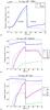 |
Fig. 6 Same as Fig. 2 for highly magnetised shocks (b = 1). nH = 102 cm-3. |
| In the text | |
|
Fig. 7 a) Atomic and b) rotational H2 lines emission for highly magnetised shocks. nH = 102 cm-3. |
| In the text | |
|
Fig. 8 Cooling normalised by kinetic power in highly magnetised shocks for a pre-shock density nH = 102 cm-3. The solid line with triangles shows the fraction of the power that is transferred into a flux of magnetic energy. |
| In the text | |
|
Fig. 9 Observed fluxes of the H2 lines in the SQ (red dots with error bars: Cluver et al. 2010, see also Table 6) with the results of our best two models. Most error bars are so small they are barely visible. |
| In the text | |
|
Fig. 10 Shape of our best two PDFs fit to the SQ data. Grey areas represent uncertainties due to the propagation of observational errors (see details in text). |
| In the text | |
|
Fig. 11 Distribution of the energy dissipated via several cooling agents for the two-Gaussian best-fit model. |
| In the text | |
Current usage metrics show cumulative count of Article Views (full-text article views including HTML views, PDF and ePub downloads, according to the available data) and Abstracts Views on Vision4Press platform.
Data correspond to usage on the plateform after 2015. The current usage metrics is available 48-96 hours after online publication and is updated daily on week days.
Initial download of the metrics may take a while.