| Issue |
A&A
Volume 549, January 2013
|
|
|---|---|---|
| Article Number | A79 | |
| Number of page(s) | 14 | |
| Section | Interstellar and circumstellar matter | |
| DOI | https://doi.org/10.1051/0004-6361/201220015 | |
| Published online | 21 December 2012 | |
Twelve type II-P supernovae seen with the eyes of Spitzer
Department of Optics and Quantum Electronics, University of Szeged, Dóm tér 9., Szeged 6720, Hungary
e-mail: This email address is being protected from spambots. You need JavaScript enabled to view it.
; This email address is being protected from spambots. You need JavaScript enabled to view it.
Received: 13 July 2012
Accepted: 5 November 2012
Abstract
Context. Core-collapse supernovae (CC SNe), especially those of type II-plateau (II-P), are thought to be important contributors to cosmic dust production. The most obvious indicator of newly-formed and/or pre-existing dust is the time-dependent mid-infrared (MIR) excess coming from the environment of SNe. In the past few years several CC SNe were monitored by the Spitzer Space Telescope in the nebular phase, hundreds of days after explosion. On the other hand, only a few of these objects have been analyzed and published to date.
Aims. Our goal was to collect publicly available, previously unpublished measurements on type II-P (or peculiar IIP) SNe from the Spitzer database. The most important aspect was to find SNe observed with the Infrared Array Camera (IRAC) on at least two epochs. The temporal changes of the observed fluxes may be indicative of the underlying supernova, while spectral energy distribution (SED) fitting to the fluxes in different IRAC channels may reveal the physical parameters of the mid-IR radiation, which is presumably caused by warm dust.
Methods. The IRS spectra were extracted and calibrated with SPICE, while photometric SEDs were assembled using IRAF and MOPEX. Calculated SEDs from observed fluxes were fit with simple dust models to obtain basic information on the dust presumed as the source of MIR radiation.
Results. We found twelve SNe that satisfied the criterion above, observed at late-time epochs (typically after +300 days). In three cases we could not identify any point source at the SN position on late-time IRAC images. We found two SNe, 2005ad and 2005af, which likely have newly formed dust in their environment, while in the other seven cases the observed MIR flux may originate from pre-existing circumstellar or interstellar dust. Our results support the previous observational conclusions that warm new dust in the environment of SNe contributes only marginally to the cosmic dust content.
Key words: supernovae: general / infrared: stars / dust, extinction
© ESO, 2012
1. Introduction
According to theoretical and observational studies during the past four decades, dust grains may be relevant components of the circumstellar matter (CSM) in the environment of core-collapse supernovae (CC SNe), which are the last stages of the life cycles of massive (M ≥ 8 M⊙) stars. However, while the possibility of dust formation around CC SNe was first raised more than 40 years ago (Cernuschi et al. 1967; Hoyle & Wickramasinghe 1970), there are still many open questions in this topic. In the local Universe, intense mass-loss processes of asymptotic giant branch (AGB) stars are thought to be the primary sources of dust. At the same time, the large observable amount of dust in high-redshift galaxies is hard to explain with AGB stars, especially because their formational timescale is longer than the age of these distant galaxies (there are some detailed reviews about this topic, see e.g. Dwek & Cherchneff 2011; Gall et al. 2011).
This is the point where CC SNe become relevant as major sources of dust in the early Universe. The lifetimes of their progenitors are usually shorter than ~1 Gyr (there are dust-rich high-z galaxies with this age, see e.g. Maiolino et al. 2004; Dwek et al. 2007). The classical models of dust production rates of CC SNe (Kozasa et al. 1989; Todini & Ferrara 2001; Nozawa et al. 2003; Morgan & Edmunds 2003) all support this theory, predicting very similar masses (0.1 − 1 M⊙) of newly formed dust. In more recent studies Bianchi & Schneider (2007); Nozawa et al. (2007); Kozasa et al. (2009); Silvia et al. (2010) also presented similar results.
An important conclusion of the latter papers is that the amount and the basic properties of the dust formed in the ejecta depend strongly on the type of the progenitor, especially the thickness of its outer H and/or He layers. As Kozasa et al. (2009) showed, a thicker outer envelope results in a lower expansion velocity and higher gas density in the deeper layers that contain the condensable elements (C, O, Mg, Al, Si). Therefore, larger ( ≥ 0.03 μm) grains are able to form. This in turn means a larger initial dust mass and also a higher survival rate of the grains. This rate is also increased by the delayed arrival of the reverse shock at the dust-forming region (because of the lower gas density in the shocked region). Based on these theoretical expectations, type II-P SNe are the best candidates for dust formation among CC SNe. Calculations of dust production efficiencies (Gall et al. 2011) also show that the mass range of 8 − 20 M⊙ (which is thought to be the typical progenitor mass range of II-P SNe) is the most important for all SNe.
However, grain formation in the expanding and cooling ejecta is not the only way to find dust around CC SNe. If there is a relatively dense CSM around the progenitor (as it is in type IIn SNe), it has probably been formed via mass-loss processes from the progenitor. This pre-existing matter also contains dust grains and may also permit grain condensation interacting with the forward shock (see more details e.g. in Fox et al. 2010, 2011).
Although the results of different models seem to be concordant, observations of CC SNe in the local Universe do not support the prediction of the intensive dust production in these objects. Optical and mid-infrared analysis of the famous SN 1987A in the Large Magellanic Cloud (LMC) revealed ~10-4 M⊙ of newly formed dust in the ejecta a few hundred days after explosion (see e.g. Danziger et al. 1989, 1991; Lucy et al. 1989, 1991; Roche et al. 1993; Wooden et al. 1993), which is orders of magnitude lower than the value predicted by theoretical studies. Similar results were found in other CC SNe studied in the past two decades based primarily on the mid-IR data of the Spitzer Space Telescope (hereafter Spitzer). None of these objects were unambigously found to have more than 0.01 M⊙ dust in their environment (see Sect. 4 for more details).
This controversy has been tried to be resolved in different ways. There is a widespread agreement that theoretical models are not perfect, and there are both micro- and macrophysical effects connected with dust formation that are not understood (see e.g. Cherchneff & Dwek 2010; Fallest et al. 2011). Circumstellar dust may form optically thick clumps (Lucy et al. 1989), resulting in a dust mass higher by an order of magnitude in numerical calculations (Sugerman et al. 2006; Ercolano et al. 2007; Fabbri et al. 2011), but it is still not a satisfying explanation. There is also a possibility that the missing dust mass is hidden in the form of cold ( ≲ 50 K) grains, whose thermal radiation is mostly invisible for Spitzer’s instruments. This cold dust should stay mainly in the SN ejecta several years after explosion, in the so-called transitional phase (Sugerman et al. 2012; Tanaka et al. 2012; Temim et al. 2012a,b), or in older supernova remnants (SNRs). Some of the nearby SNRs were observed at mid-IR, far-IR, and submillimeter (sub-mm) wavelengths, but the inferred dust masses vary on a large scale (from 10-4 to 1 M⊙), sometimes even for the same object (see the review of Gall et al. 2011). Recently, observations from the Herschel Space Observatory are expected to give reassuring answers. The published results suggest relatively large dust masses: 0.08 M⊙ in Cas A (Barlow et al. 2010), 0.1−10 M⊙ in N49 in the LMC (Otsuka et al. 2010), and 0.4−0.7 M⊙ in SN 1987A (Matsuura et al. 2011); although new measurements on SN 1987A made with the Atacama Pathfinder EXperiment (APEX) at sub-mm wavelengths do not support the presence of such a large amount of dust (Lakicevic et al 2012).
There are also some other ideas, but they are not supported by any convincing observational evidence. The observed low dust production rates of CC SNe could be compensated with a top-heavy initial mass function (IMF), which might be a characteristic of some early galaxies (e.g. Bromm et al. 2002; Tumlinson 2006; Michalowski et al. 2010). It is also possible that pair-instability supernovae (PISNe), the assumed fate of stars with progenitor masses of 140 − 260 M⊙ (Heger et al. 2003), could be efficient dust producers in the first galaxies (Nozawa et al. 2003; Gall et al. 2011), but there are still no strong evidence for the existence of these objects. Some authors argue that depending on star-formation history, AGB stars may be significant dust sources in galaxies younger than 1 Gyr (Valiante et al. 2009; Dwek & Cherchneff 2011). There is another interesting idea about possible grain condensation in quasar winds (Elvis et al. 2002). Beyond these ideas, more calculations suggest significant grain growth in the ISM, which may be an acceptable explanation of both the low dust production rates of SNe and the high dust content of distant galaxies (Draine 2003, 2009; Michalowski et al. 2010; Mattsson & Andersen 2012; Mattsson et al. 2012).
To get closer to the mystery of the origin of cosmic dust, it is necessary to have a large amount of high-quality observational data. Up to now, there are only 20−25 SNe for which we have quantitative pieces of information about their dust content; see e.g. Fox et al. (2011), Gall et al. (2011), Szalai et al. (2011), and Sect. 4 for details. Regarding the type II-P SNe, there are less than ten objects with detailed analyses, and we know quite a few examples without detectable dust content. Fox et al. (2011) published the results of a survey to detect MIR excess (the most obvious evidence of warm dust) in the environment of type IIn SNe. They found late-time emission in ten objects from their sample of 69 SNe and concluded that the IIn subclass represents the largest part of dust-containing SNe (it should be noted that the authors carried out this project during the warm mission of Spitzer, so they were able to use only the 3.6 and 4.5 μm channels supplemented by optical and near-IR photometry and spectroscopy).
Motivated partly by the work of Fox et al. (2011), our goal is to perform such analyses for type II-P SNe that are thought to be the best candidates for producing newly formed dust. We collect, reduce, and analyze unpublished measurements on CC SNe belonging to the II-P subclass, found in the public Spitzer database. In Sect. 2 we show the steps of data reduction and present the extracted photometric and spectroscopic data. We present observed spectral energy distributions (SEDs) of the studied SNe, and compare them with different dust models (Sect. 3). We note that although the properties of the cold ISM are better constrained by far-IR and/or sub-mm data, the low angular resolution of the available instruments prevent measurements of extragalactic SNe. The Spitzer data we applied in this paper probe only the warm (T ~ 200−1000 K) dust in the environment of extragalactic SNe. Thus, our study focuses on the presence/absence of warm dust and its physical properties. We discuss the results of the SED fitting in Sect. 3.2. Finally, we summarize our results and conlusions, and give a brief discussion on the role of type II-P SNe in cosmic dust production.
2. Observations and data reduction
We queried the public Spitzer database to find type II-P SNe observed with the Infrared Array Camera (IRAC) on at least two epochs. We found 12 SNe satisfying this criterion. We also collected observations obtained by Spitzer’s Multiband Imaging Spectrometer (MIPS) and Infrared Spectrograph (IRS) instruments (not only the spectra but also the broad-band photometric data recorded in peak-up imaging mode, PUI). In addition, we also checked the literature for any other observational data obtained around the same epoch as the Spitzer measurements.
2.1. Supernova sample observed by Spitzer
Basic data of the supernovae.
SN 2003J was discovered in NGC 4157 on 2003 January 11.3 UT (dates are in UT thereafter) by Kushida et al. (2003; ~16.7 mag, unfiltered). Ayani et al. (2003) classified 2003J as a normal type-II SN. Using the infrared map of Schlegel et al. (1998), the calculated value of galactic interstellar reddening is E(B − V)gal = 0.021 mag. The estimated distance (D) to the host galaxy (based on surface brightness fluctuations) is 14.7 Mpc (Tonry et al. 2001).
SN 2003hn was discovered in NGC 1448 on 2003 August 25.7 by Evans et al. (2003; V ~ 14.4 mag). Preliminary spectroscopic analysis by Salvo et al. (2003) showed that 2003hn was a type II-P supernova. Detailed analysis based on optical and near-infrared photometry and optical spectroscopy was carried out by Krisciunas et al. (2009), while Jones et al. (2009) and Olivares et al. (2010) also analyzed the data of SN 2003hn and of other type II-P SNe to obtain precise distances to the host galaxies. We adopt 18.1 Mpc as the distance of the SN (Krisciunas et al. 2009) and t0 = JD 2 452 859 as the moment of explosion (Jones et al. 2009), while we use E(B − V)total = 0.19 mag as the estimated reddening of the host galaxy (Olivares et al. 2010).
SN 2003ie was discovered in NGC 4051 on 2003 September 19.8 (Arbour & Boles 2003) with an apparent brightness of ~15.0 mag (unfiltered). Benetti et al. (2003) classified it as a type-II SN, while Harutyunyan et al. (2008) found similarities between some spectral features of SN 2003ie and the peculiar type II-P SNe 1998A and 1987A. Based on data on both the SN and its host galaxy (distance, metallicity, extinction) Smartt et al. (2009) gave 25 M⊙ as an upper limit for its progenitor mass. For our studies we adopt D = 15.5 Mpc (Pierce & Tully 1988; Smartt et al. 2009), E(B − V)gal = 0.013 mag (Schlegel et al. 1998), and t0 = 2 452 868 (Harutyunyan et al. 2008).
SN 2004A was discovered in NGC 6207 on 2004 January 9.8 by the Japanese amateur astronomer K. Itagaki (see Nakano et al. 2004) with a brightness of ~15.7 mag (unfiltered). A preliminary optical spectrum obtained by Kawakita et al. (2004) indicated that it was a type-II SN. Based on their detailed optical photometric and spectroscopic analysis, Hendry et al. (2006) found 2004A to be a classical type II-P SN with D = 20.3 Mpc, E(B − V)total = 0.06 mag, and t0 = 2 453 011. Maguire et al. (2010) also published optical photometric and spectroscopic data from the photospheric phase.
SN 2005ad was discovered in NGC 941 on 2005 February 6.4 by K. Itagaki on unfiltered CCD-images (see Nakano & Itagaki 2005) with a brightness of ~17.4 mag. The very blue continuum on early spectra (Morrell et al. 2005) indicated that 2005ad was discovered in a very early phase, but the exact value of t0 is still unknown. Lacking detailed studies, classification of 2005ad is difficult, but some authors (Smartt et al. 2009; Li et al. 2011) refer to it as a type II-P SN. We use the values of D = 20.8 Mpc (Li et al. 2011) and E(B − V)gal = 0.06 mag (Schlegel et al. 1998).
SN 2005af appeared in the nearby galaxy NGC 4945 on 2005 February 8.2 with an apparent brightness of V = 12.8 mag (Jacques & Pimentel 2005). Spectroscopic analysis of Filippenko & Foley (2005) showed that it was a normal type II-P event. Pereyra et al. (2006) obtained optical polarimetry during the photospheric and the early nebular phase, while Kotak et al. (2006) and Kotak (2008) reported mid-IR data from this period (see details below). From the latter study we adopt D = 3.9 Mpc and t0 = 2 453 379, and use E(B − V)gal = 0.183 mag for reddening (Schlegel et al. 1998).
SN 2005cs was discovered in the nearby, spectacular Whirlpool Galaxy (M51, NGC 5194) on 2005 June 28.9 by Kloehr et al. (2005). It was classified as a type-II SN by Modjaz et al. (2005). Because of its proximity, it was the target of many observing campaigns. Early-time optical photometry and spectroscopy were presented by Pastorello et al. (2006) and Dessart et al. (2008), while Brown et al. (2007) studied the SN using the Swift ultraviolet-optical and X-ray telescopes. SN 2005cs seems to belong to the subtype of low-luminosity, 56Ni-poor, low-velocity SNe II-P, as shown also by long-term studies of Tsvetkov et al. (2006; optical photometry), Gnedin et al. (2007; R-band photometry and polarimetry), and Pastorello et al. (2009; optical and near-IR photometry, optical spectroscopy). Extensive studies of the first-year data and pre-explosion images resulted in a progenitor mass of 7−13 M⊙ (Maund et al. 2005; Li et al. 2006; Takáts & Vinkó 2006; Eldridge et al. 2007), while Utrobin & Chugai (2008) determined a significantly higher value (17−19 M⊙). In their more recent work Pastorello et al. (2009) concluded that the progenitor mass should be in the range of 10−15 M⊙. The distance to the host galaxy, determined via different methods, is scattered between 5.9–9.4 Mpc (Feldmeier et al. 1997; Pastorello et al. 2006; Takáts & Vinkó 2006; Dessart et al. 2008). Recently, Vinkó et al. (2012) determined its mean value of 8.4 Mpc by combining the data of SNe 2005cs and 2011dh in the same galaxy. We adopt this latter value for D as well as t0 = 2 453 550 (Pastorello et al. 2006), and E(B − V)total = 0.04 mag (Baron et al. 2007; Dessart et al. 2008).
SN 2006bc was discovered in NGC 2397 by R. Martin (see Monard et al. 2006) on 2006 March 24.6; its apparent brightness was 16.0 mag (on an unfiltered CCD-image). Early spectra clearly showed that it was a type-II SN (Patat et al. 2006), but due to the lack of long-term studies it remains unsolved whether it is a II-P or a II-L SN (Smartt et al. 2009; Otsuka et al. 2012). While Smartt et al. (2009) could not identify the progenitor of 2006bc on Hubble Space Telescope (HST) archive images, Otsuka et al. (2012) also used HST to obtain late-time optical photometry. Brown et al. (2009) also observed it with the Swift UVOT detector. Parallel to our work, Gallagher et al. (2012) carried out a complete optical and infrared analysis (see details below). The distance to the host galaxy, D = 14.7 Mpc, is only estimated from its kinematic motion (Smartt et al. 2009). We also adopt E(B − V)gal = 0.205 mag (Schlegel et al. 1998), and t0 = 2 453 819 (Gallagher et al. 2012).
SN 2006bp, appearing in NGC 3953, was found by K. Itagaki (see Nakano & Itagaki 2006a) on 2006 April, 9.6 (16.7 mag, unfiltered). Early spectroscopic (Quimby et al. 2006, 2007; Dessart et al. 2008) and photometric observations – in optical (Quimby et al. 2007; Dessart et al. 2008), UV and X-ray (Immler et al. 2007; Dessart et al. 2008; Brown et al. 2009) – showed that 2006bp was a classical type II-P SN, and it was discovered only a few hours after shock breakout, which is the earliest discovery among type II-P SNe. Adopting the results of Dessart et al. (2008), we used the data D = 17.5 Mpc, E(B − V)total = 0.400 mag, and t0 = 2 453 833.
SN 2006my was discovered in NGC 4651 by K. Itagaki (see Nakano & Itagaki 2006b) on 2006 November 8.8 with an apparent unfiltered brightness of 15.3 mag, well past maximum light. Analyzing the first spectra after discovery, Stanishev & Nielsen (2006) classified it as a type II-P SN. Li et al. (2007) and Maguire et al. (2010) carried out optical photometric and spectroscopic observations both in the photospheric and in the early nebular phase. From optical spectropolarimetry, Chornock et al. (2010) showed strong late-time asphericities in the inner core of 2006my. Extended studies, based on the analysis of pre- and post-explosion images of HST and high-resolution ground-based telescopes, concluded that the progenitor of the SN should have been a red supergiant with a mass between 7–13 M⊙ (Li et al. 2007; Leonard et al 2008; Smartt et al. 2009; Crockett et al. 2011). Solanes et al. (2002) reported D = 22.3 Mpc as the distance of the host galaxy; we used this value, as well as t0 = 2 453 943 as the moment of explosion (Maguire et al. 2010) and E(B − V)gal = 0.027 mag as galactic reddening (Schlegel et al. 1998).
SN 2006ov, appearing in NGC 4303, has many similarities with 2006my. It was also found by K. Itagaki (see Nakano & Itagaki 2006c) on 2006 November 24.9. Its unfiltered apparent brightness was 14.9 mag at the moment of discovery. Similarly to 2006my, 2006ov was a type II-P SN discovered near the end of the plateau phase (Blondin et al. 2006; Li et al. 2007). It was also one of the three CC SNe in which Chornock et al. (2010) found late-time asphericity in the inner ejecta. Li et al. (2007) determined the mass of the progenitor as 15 , but later works (Smartt et al. 2009; Crockett et al. 2011) gave 10 M⊙ as an upper limit. We adopt D = 12.6 Mpc (Smartt et al. 2009) and E(B − V)gal = 0.022 mag (Schlegel et al. 1998), while we estimated t0 = 2 453 964 based on the results of Li et al. (2007).
SN 2007oc was discovered in NGC 7418A on 2007 November 3.1 by the Chilean Automatic Supernova Search program (Pignata et al. 2007). Due to the lack of any published photometric or spectroscopic observations, the moment of explosion and its subtype remain unknown; it is mentioned in the ASIAGO Supernova Catalogue as a type II-P SN (Barbon et al. 2008). We adopted D = 28.0 Mpc as the distance of the host galaxy (Gil de Paz et al. 2007) and E(B − V)gal = 0.023 mag (Schlegel et al. 1998) as the galactic reddening.
2.2. Mid-infrared photometry with Spitzer
We collected and analyzed all available IRAC post-basic calibrated data (PBCD) on the 12 CC SNe listed above. The scale of those images is 0.6″/pixel. In some cases, a clear identification of SN was not easy because of the faintness of the target in the vicinity of bright regions. We tried to apply the image-subtraction technique used succesfully in some cases to analyze Spitzer data of SNe (Meikle et al. 2006, 2007; Kotak et al. 2009). We found pre-explosion images of the host galaxies for only two SNe (2005cs and 2006ov), and their quality was too poor for reliable image subtraction. We also generated some subtracted images using the latest frames as templates, but their applicability was also very limited. Finally, we were able to unambiguously identify a MIR point source in nine cases at the SN position, while in the cases of three SNe (2003hn, 2005cs, and 2006bc) we did not find any sign of a point source, either on the original images or on the subtracted image (however, as we mentioned before, there are some other recent results about SN 2006bc, see details in Sect. 4). For the nine detected SNe (Fig. 1) we carried out a detailed photometric analysis.
Originally, we planned to apply PSF-photometry using the DAOPHOT package of IRAF1 to obtain more accurate results. Unfortunately, the bright background flux of the host galaxies, sometimes showing rapid spatial variations, and the lack of relatively bright point sources on the frames prevented us from applying this.
Therefore we carried out simple aperture photometry on the PBCD frames with the PHOT task of the IRAF software package. This was possible beacuse the studied SNe – except of the three mentioned above – were clearly identifiable on IRAC images (see Fig. 1). We generally used an aperture radius of 3.6′′ and a background annulus from 3.6′′ to 8.4′′ (3-3-7 configuration in native ~1.2′′ IRAC pixels), applied aperture corrections of 1.124, 1.127, 1.143, and 1.234 for the four IRAC channels (3.6, 4.5, 5.8, and 8.0 μm) as given in the IRAC Data Handbook (Reach et al. 2006). We chose a 2-2-6 configuration for SNe 2003J and 2007oc (aperture corrections: 1.213, 1.234, 1.379, and 1.584), and a 5-12-20 configuration on the images of the bright, nearby SN 2005af (aperture corrections: 1.049, 1.050, 1.058, and 1.068).
There is one object, 2005af, for which MIR data were partly analyzed and published before: Kotak et al. (2006) presented IRS spectra and also IRAC and PUI fluxes up to +433 days, while in Kotak (2008) there is a figure showing an IRS spectrum and IRAC measurements carried out at +571 days. To check the reliability of our reduction technique we also reduced these data and found a good agreement with the results of Kotak et al. (2006) and Kotak (2008). We also completed this dataset with the fluxes determined from the latest measurements found in the Spitzer database.
We also carried out aperture photometry using IRAF on late-time MIPS 24.0 μm PBCD frames (image scale 2.45′′/pixel) for SNe 2003J, 2003ie, 2005af, 2006bp, and 2006my. We used an aperture radius of 3.5′′ and a background annulus from 6′′ to 8′′, except for SN 2005af, for which we found the 5-5-12 configuration to be the best choice. For SNe 2005af and 2006my, the MIR point sources were also identifiable on available IRS PUI images. Their fluxes were measured using the MOsaicker and Point source EXtractor (MOPEX2) software. All measured fluxes are listed in Table A.1.
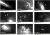 |
Fig. 1 Type II-P SNe on IRAC post-BCD 4.5 μm images. The FOV is 100′′ × 60′′. North is up, and east is to the left. |
2.3. Mid-infrared spectroscopy with IRS
We also downloaded the available IRS spectra of the SNe from the Spitzer database. Four spectra of SN 2005af – the first three have already been published by Kotak et al. (2006) and Kotak (2008) –, two spectra of SN 2004A, and a single spectrum of SNe 2003ie, 2005ad, 2005cs, 2006bp, and 2006ov were collected this way.
IRS observations of the SNe.
We analyzed the PBCD-frames of the spectroscopic data with the Spitzer IRS Custom Extraction software (SPICE3). Sky subtraction and bad pixel removal were performed using two exposures that contained the spectrum at different locations, which were then subtracted them from each other. Order extraction, wavelength- and flux-calibration were performed by applying built-in templates within SPICE. Finally, the spectra from the first, second and third orders were combined into a single spectrum with the overlapping edges averaged. In a few cases the sky near the order edges was oversubtracted because of some excess fluxes close to the source, which resulted in spurious negative flux values in the extracted spectrum. These were filtered out using the fluxes in the same wavelength region that were extracted from the adjacent orders.
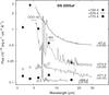 |
Fig. 2 IRS spectra of SN 2005af. The spectra at different epochs are vertically shifted relative to each other by the amount indicated in the labels next to the spectra. |
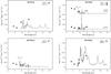 |
Fig. 3 IRS spectra of SNe 2003ie, 2004A, 2005ad, and 2006bp. The spectra of SN 2004A are vertically shifted relative to each other by the amount indicated in the label next to the upper spectrum. Strong and wide emission features in the spectrum of SN 2006bp possibly emerge from nearby interstellar clouds. |
We found that the spectra of SNe 2005cs and 2006ov are too noisy for further analysis. For the other SNe the spectral and photometric fluxes agree reasonably well. We also compared the extracted spectra with the public data in the Cornell Atlas of Spitzer IRS Sources4 (CASSIS, Lebouteiller et al. 2011), and found them to be similar to each other.
The spectra of SN 2005af are shown in Fig. 2. The three earliest spectra were already published by Kotak et al. (2006) and Kotak (2008). Our spectra agree well with theirs, which serves as a good test for checking our data reduction. In Fig. 3 we present the extracted IRS spectra for the other SNe. Although detailed modeling of these spectra is beyond the scope of this paper, we identified spectral features of SiO, and the 1−0 vibrational transition of CO based on line identifications of Kotak et al. (2005, 2006). The SiO feature plays an important role in modeling the observed SEDs, while the CO 1−0 transition results in a flux excess at 4.5 micron (see Sect. 3).
3. Analysis
3.1. Mid-IR SEDs
Figure 4 shows the mid-IR SEDs of the SNe calculated from IRAC 3.6, 4.5, 5.8, and 8.0 μm fluxes (plotted with available PUI 13.0 − 18.5 μm and MIPS 24.0 μm fluxes). The continuum fluxes of the reduced IRS spectra match the SED flux levels well.
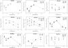 |
Fig. 4 Mid-IR SEDs of the nine CC SNe at different epochs. Open symbols denote IRAC warm mission data. |
As is seen in Fig. 4, IRAC fluxes of several SNe (2003J, 2004A, 2005ad, 2005af, 2007oc) show obvious variations in time, while others do not. Based on the analysis of other CC SNe, e.g., SN 2004et (Kotak et al. 2009) or SN 2004dj (Szalai et al. 2011; Meikle et al. 2011), this temporal evolution could be the sign of newly-formed dust grains in the ejecta, but there may be more effects that have to be taken into account to explain this phenomenon.
3.2. Fitting of dust models to MIR SEDs
Assuming that the radiation is purely thermal, the main source of mid-IR flux is most likely warm dust. To estimate the minimum amount of dust, we fit analytic dust models to the observed SEDs. Prior to fitting, the observed SED fluxes were dereddened using the galactic reddening law parametrized by Fitzpatrick & Massa (2007) assuming RV = 3.1 and adopting E(B − V) values as listed in Sect. 2.1.
As a first step we examined whether simple, pure blackbody (BB) emission might be consistent with the observed MIR SEDs. Although a pure BB model has little physical significance, we applied it to estimate the minimum radius of an optically thick dust sphere that fits the observed SEDs. From the minimum radii we calculated the corresponding velocities assuming homologous expansion (see Table 3). The typical velocities of type II-P SNe are 2−3000 km s-1 for the inner ejecta where dust formation may take place. Therefore, for a larger minimum size it is not possible that the inner ejecta reach the calculated size of the BB. This means that in these cases the minimum radii of the optically thick dust spheres are too large and that consequently, most of the estimated dust mass cannot have originated from newly formed grains.
Minimum radii and corresponding velocities determined from the best-fit BB-models to observed SEDs.
The analytic models were calculated using Eq. (1) in Meikle et al. (2007) assuming a homogeneous (constant-density) dust distribution: ![Mathematical equation: \begin{equation} L_{\nu}=2 \pi^2 R^2 B_{\nu}(T)\left[ \tau_{\nu}^{-2} (2\tau_{\nu}^2 -1 + (2 \tau_{\nu} + 1)\exp(-2 \tau_{\nu}) \right], \end{equation}](/articles/aa/full_html/2013/01/aa20015-12/aa20015-12-eq60.png) (1)where R is the radius of the dust sphere, Bν(T) is the Planck function, T is the temperature of the dust, and τν is the optical depth at a given frequency. To estimate the dust optical depth, we adopted the power-law grain-size distribution of Mathis et al. (1977, hereafter MRN), assuming m = 3.5 for the power-law index and grain sizes between amin = 0.005 μm and amax = 0.05 μm. τν can then be calculated as
(1)where R is the radius of the dust sphere, Bν(T) is the Planck function, T is the temperature of the dust, and τν is the optical depth at a given frequency. To estimate the dust optical depth, we adopted the power-law grain-size distribution of Mathis et al. (1977, hereafter MRN), assuming m = 3.5 for the power-law index and grain sizes between amin = 0.005 μm and amax = 0.05 μm. τν can then be calculated as ![Mathematical equation: \begin{equation} \tau_{\nu} = \frac{4}{3} \pi k \rho_{\rm grain} \kappa_{\nu} R \frac{1}{4-m} \left[ a^{4-m}_{\max} - a^{4-m}_{\min} \right], \end{equation}](/articles/aa/full_html/2013/01/aa20015-12/aa20015-12-eq67.png) (2)where ρgrain is the density of dust grain material, k is the grain number-density scaling factor, and κν is the mass absorption coefficient. The dust is assumed to be distributed uniformly within a sphere. R, T, and k were free parameters during the fitting.
(2)where ρgrain is the density of dust grain material, k is the grain number-density scaling factor, and κν is the mass absorption coefficient. The dust is assumed to be distributed uniformly within a sphere. R, T, and k were free parameters during the fitting.
First we calculated the dust models using amorphous carbon (AC) grains. Dust opacity values were taken from Colangeli et al. (1995), while the density of the dust grain material, ρgrain = 1.85 g cm-3, was adopted from Rouleau & Martin (1991). Although we were able to successfully apply these models in most cases, finding adequate solutions for SNe 2005af and 2006my was possible only by assuming silicate dust (C-Si-PAH mixture, MRN-distribution, ρgrain = 3.00 g cm-3, Weingartner & Draine 2001). The IRS spectra of SN 2005af also show the signs of SiO (see Sect. 2 and Kotak et al. 2006); but there were no IRS spectra on SN 2006my in the database. On the other hand, the spectra of the other SNe (2003ie, 2004A, 2005ad, 2006bp) that can be fit well with AC models do not show obvious signs of SiO. The parameters of the best-fit analytic models (shown in Fig. 5) are collected in Tables 4 and 5.
Parameters for the best-fit analytic amorphous carbon dust models to the warm components of SEDs.
Parameters for the best-fit analytic silicate dust models to the warm components of SEDs.
In a few cases we found that a single temperature model cannot describe the whole observed SED. This is similar to the result of Wooden et al. (1993), who showed that for SN 1987A a hot component (T ~ 5 − 10 000 K) may affect the continuum emission of the warm dust. This hot component is thought to be caused by an optically thick gas in the innermost part of the ejecta. The contribution of such a hot component can be significant at shorter IRAC wavelengths. The modeling of the hot component needs late-time optical or near-IR data taken simultaneously with the Spitzer observations. Because of the lack of such data for most of the SNe in our sample, we usually did not include the 3.6 μm (and sometimes also 4.5 μm) fluxes while fitting the dust models. There are two exceptions for which we have found optical photometry obtained close to the IRAC measurements: SN 2004A at 247 days (Hendry et al. 2006), and SN 2006my at 205 days (Maguire et al. 2010). At these epochs we completed the observed SEDs with the optical data and added a hot component to our models (see the fittings in Fig. 6, and the parameters in Table 6.).
Figure 5 shows that SNe 2004A, 2005ad, 2005af, and 2007oc show variable excess flux at 4.5 μm (in these cases we omitted the 4.5 μm fluxes from the fitting). The excess flux weakens with age, as the ejecta temperature decreases. This trend is also seen in the IRS spectra of SN 2005af (see Sect. 2 and Kotak et al. 2006). This may be due to the influence of the red wing of the 1 − 0 vibrational transition of CO at 4.65 μm (see also Kotak et al. 2005, 2006; Szalai et al. 2011). An alternative explanation for temporarily changing flux at 4.5 μm may be the rapid destruction of stochastically heated grains. This effect becomes significant when the grain sizes are below 0.003 μm (Bocchio et al. 2012). However, as we mentioned above, in the cases studied here the grain sizes are thought to be more than 0.005 μm (see also Sect. 1, and Kozasa et al. 2009; Szalai et al. 2011). Therefore the rapid grain destruction process seems to be less significant around these young SNe than it might be in older SNRs.
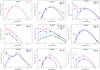 |
Fig. 5 Best-fit analytic models on MIR SEDs of the SNe. The 3.6 μm and sometimes the 4.5 μm fluxes are usually not included in the fitting (see text). The fittings that contain hot and warm components for SN 2004A and SN 2006my are shown in Fig. 6. |
We also found that single-temperature models underestimate the fluxes at 24 μm when there are MIPS data taken contemporaneously with the IRAC measurements (SNe 2003ie, 2006bp, 2006my). In these cases we added a cold component (T ~ 100 K) to our models, similar to Kotak et al. (2009) and Szalai et al. (2011), which resulted in a reasonably good fit to the whole observed SED. The parameters of the cold BBs are collected in Table 6.
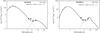 |
Fig. 6 Best-fit models for SN 2004A at 247 days (left) and for SN 2006my at 205 days (right) that contain a warm dust component and a hot blackbody (see text). |
The calculated dust masses for all SNe and all epochs are also collected in Tables 4 and 5. Masses were determined using the formula  (3)adopted from \citet{Lucy89} and \citet{Meikle07}. It should be noted that these masses from analytic models are lowerlimits (Meikle et al. 2007), because of the implicit assumption that the dust cloud has the lowest possible optical depth. As mentioned before, more realistic dust masses can be obtained only from numerical models for the optically thick dust cloud.
Parameters of the additional cold and hot blackbodies.
To check this statement and the trustworthiness of our analytic model fitting, we generated some models with the three-dimensional radiative-transfer code MOCASSIN 2.02.55. (Ercolano et al. 2003, 2005). This numerical code uses a ray-tracing technique, following the paths of photons emitted from a given source through a spherical shell containing a specified medium. The shell is mapped onto a Cartesian grid allowing light-matter interactions (absorption, re-emission, and scattering events) and to track energy packets until they leave the shell and contribute to the observed SED. It is applicable for reconstructing dust-enriched environments of CC SNe and to determine physical parameters such as grain-size distribution, composition, and mass of dust (see Sugerman et al. 2006; Ercolano et al. 2007; Fabbri et al. 2011; Szalai et al. 2011). The code handles different types of dust heating processes caused not only by photons but also by collisions of grains and electrons (B. Ercolano, pers. comm.).
Parameters for the best-fit MOCASSIN models to SN 2005af SED at +576 days.
We chose SN 2005af as a test object (at 576 days), for which we could fit both AC and Si-containing dust models. For AC grain composition we used the built-in optical constants from Hanner (1988), while to fit also the flux at 8 μm we found a 0.65:0.35 Si-AC mixture to be the best solution (built-in optical constants of astronomical silicate are taken from Laor & Draine 1993). We applied the MRN grain-size distribution. The final results of numerical calculations are shown in Table 7, while we compare the best-fitting analytical and numerical models in Fig. 7. The excess flux below 3 μm in the MOCASSIN model comes from the assumed hot central source, which was absent in the analytic models.
Although the two methods are very different (the analytic models describe the thermal MIR radiation of the dust, while the calculations of MOCASSIN are based on more detailed radiative transfer), we were able to generate similar SEDs in the MIR region with similar dust shell sizes. For pure AC dust, dust mass derived with the numerical model is an order of magnitude higher than that derived with the analytical model, which is very similar to our earlier results on SN 2004dj (Szalai et al. 2011). Models for silicate dust are slightly different in numerical and in analytic models, and, to obtain the best fit, we had to apply larger grains (a = 0.1−1 μm, MRN distribution). Despite these differences, the calculated mass for the silicate dust shell is very close to the value given by the analytic model.
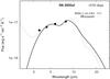 |
Fig. 7 Best-fitting Si-containing analytical and numerical models for SN 2005af at +576 days (solid and dotted lines, respectively). The excess flux below 3 μm in the MOCASSIN model is due to the assumed hot central source, which was absent from the analytic models. |
4. Discussion
To understand the origin and heating mechanisms of dust in the environment of SNe, it is important to combine the MIR data with optical and/or near-IR measurements (see e.g. Kotak et al. 2009; Fox et al. 2010; Otsuka et al. 2010; Szalai et al. 2011; Meikle et al. 2011). Observations in X-ray and radio may also provide useful additional information about SN-CSM interactions. However, while Spitzer observations on the studied SNe were typically carried out in the nebular phase, there are only a very few additional late-time observations of these objects (see these cases above). Therefore, we can draw our conclusions based on mainly the MIR data analyzed in the previous section.
As mentioned before, there are three SNe in our sample (2003hn, 2005cs, and 2006bc) for which the available MIR data were not appropriate to resolve the point source at the position of the SN. The case of SN 2006bc is special, because there is a bright source (probably a surrounding H II region) very close to the position of the SN. One would need high-resolution data and more sophisticated methods to extract information on this SN (Otsuka et al. 2012). Parallel to our studies, Gallagher et al. (2012) carried out a complete optical and infrared data analysis of SN 2006bc based not only on Spitzer observations but also HST and Gemini South data. They found Mdust ≤ 2 × 10⁻³ M⊙ newly formed dust in the ejecta, which is consistent with other similar cases.
The SEDs of the studied SNe and the derived parameters shown in Tables 3−5 give guidelines and limits to the possible sources of the detected MIR radiation. We have the highest amount of data for SN 2005af, for which a sequence of MIR SEDs is available that shows a monotonically decreasing temperature (see Fig. 4). This may be the sign of newly formed, cooling dust. It is also supported by the size of the dust sphere determined from the models: the calculated expansion velocities are lower than 1300 km s-1 in the nebular phase, which is low enough to be compatible with the inner ejecta velocities of II-P SNe. This is clearly another argument that most of the dust may have been formed in the ejecta. The calculated dust masses (1−3 × 10⁻⁴ M⊙) agree with the amount of SiO calculated by Kotak et al. (2006) and with the results of Kotak (2008), and they are also similar to the values found in other SNe.
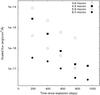 |
Fig. 8 IRAC light curves of SN 2005af: 3.6 μm (open squares), 4.5 μm (filled squares), 5.4 μm (open circles), 8.0 μm (filled circles). |
Another explanation for the observed behavior of MIR SEDs may be the thermal radiation of pre-existing dust in the CSM re-heated by the SN, i.e., the IR-echo (Bode & Evans 1980; Dwek 1983, 1985; Sugerman 2003). We have very little information on the properties of the CSM around this SN. There are no published X-ray or radio measurements, and the relatively high value of the interstellar reddening (E(B − V)gal = 0.183 mag) is caused by the galactic ISM. However, based on Dwek (1983) and Meikle et al. (2006), the shapes of the MIR light curves should be rather flat if there is an IR echo, but the IRAC light curves of SN 2005af decline monotonically in time (see Fig. 8). Therefore we conclude that an IR echo is a less probable source of MIR radiation during the observed interval. It is also possible that dust grains condense in a cool dense shell (CDS) that is generated between the forward and reverse shock waves during the interaction of the SN ejecta and the pre-existing CSM. This is usually invoked for type IIn SNe, but it was also taken into account in a few other cases to explain the presence of early or very late MIR-excess (Kotak et al. 2009; Andrews et al. 2010; Meikle et al. 2011). A CDS was also assumed to be the source of the cold dust component in the SEDs of II-P SNe (Szalai et al. 2011).
The shapes of the MIR light curves and the presence of SiO make SN 2005af very similar to the well-studied SN 2004et. In this SN the main source of the warm component is also identified as cooling, newly formed dust in the ejecta (Kotak et al. 2009). Unfortunately, there are no Spitzer measurements on SN 2005af at very late epochs, so we could not see whether there is also a rise in IRAC fluxes after +1000 days like in SN 2004et (Kotak et al. 2009; Fabbri et al. 2011).
List of type II-P supernovae with published Spitzer data.
There are fewer Spitzer data for the other eight SNe, and some of them were recorded during the warm mission (since the end of the cryogenic mission in 2009 only the IRAC 3.6 and 4.5 μm channels have been usable). Nevertheless, we may also draw some conclusions for these SNe. Among them we found obvious MIR flux changes in four objects: SNe 2003J, 2004A, 2005ad, and 2007oc (we note that for SN 2003J there is only one complete IRAC measurement, the second one was made during the warm mission). From these, SN 2005ad is the only object for which calculated parameters may indicate dust formation with high probability, because between the two observed epochs the dust model temperature decreased from 890 K to 750 K. The calculated expansion velocities are even lower than for SN 2005af, and the calculated dust masses (~10-5 M⊙) also agree with the values found in similar cases. Interestingly, for both SNe 2005af and 2005ad, the calculated radii of the dust sphere are roughly constant (or decline slightly) in the nebular phase in spite of the expected expansion. Kotak et al. (2009) found a similar effect in SN 2004et: their explanation was that the dust was contained within an optically thin cloud of optically thick dust clumps that cannot move outward because of the hotter, higher pressure interclump gas.
While the flux changes of SNe 2003J, 2004A, and 2007oc suggest that the observed MIR radiation is connected to the SN (at least partly), only a part of it may have been emitted by newly formed grains in the ejecta. The derived dust sphere radii indicate very high expansion velocities that are much higher than the inner ejecta velocities of type II-P SNe in the nebular phase. At such large radii grain condensation is unlikely. SN 2004A shows changes in the dust temperature, and the calculated luminosities of the dust spheres are not much higher than for SNe 2005af and 2005ad, but the source of most of the MIR radiation may be pre-existing dust or the bulk of grains formed in a CDS. This may be even more valid for SNe 2003J and 2007oc.
For the remaining four SNe (2003ie, 2006bp, 2006my, 2006ov) there is no sign of real changes in the detected MIR fluxes. However, model fits to their SEDs suggest very high expansion velocities and much larger dust masses than for SNe 2005af and 2005ad (note that these values are still lower than the theoretically predicted dust masses). While this does not completely rule out that there is newly formed or pre-existing dust in the close environment of these SNe, the amount of dust should be smaller than the calculated values. We conclude that there are probably other sources of MIR radiation, e.g., dust and/or cold gas clouds within the host galaxies or in the line-of-sight of these SNe. For SN 2006bp, the high value of reddening, E(B − V)total = 0.4 mag, supports this idea. For the other three SNe the E(B − V) values are much lower but are estimated only from the galactic reddening map of Schlegel et al. (1998). We also note that the 3″ aperture radii used by IRAC photometry correspond to 20−35 pc at the distances of our SNe, which is 2−3 orders of magnitude larger than the regions that the SN ejecta or shock waves could achieve at the given epochs (it may be less valid for SN 2005af, which is much closer than the other SNe in the sample).
In Table 8 we show all type II-P SNe that have Spitzer data analyzed and published to date including the objects presented in this work. As the final list shows, we doubled the number of objects, which might serve as a basis for statistical studies on a larger sample. We separated SNe that have some amount of local dust from those where there is no unambiguous sign for dust. Similar tables about the dust formation statistics of SNe can be found for instance in Fox et al. (2011) and Gall et al. (2011).
5. Summary
We collected the public photometric and spectroscopic data of the Spitzer on 12 type II-P SNe. We found the data of nine of these objects to be appropriate for a detailed study, which almost doubles the number of type II-P SNe with a detailed, published MIR data analysis. We fit the observed SEDs with simplified one- or two-component dust models. In SNe 2005ad and 2005af we found cooling temperatures and decreasing luminosities of the warm component that are similar to the values found in other SNe that are thought to have newly formed dust in their environment.
The calculated temperatures for the other SNe do not show strong temporal variation, while the derived luminosities and radii are too high to be compatible with local dust. Moreover, the calculated dust masses in these cases are orders of magnitude higher than the observed amount of dust around the well-studied SNe listed above. The large radius of the warm component may suggest pre-existing dust in these cases, making it unclear if there was new dust formed around these SNe. Nevertheless, theoretical models predict orders of magnitude more newly formed dust in CC SNe. Our conclusions support the previous observational results that warm new dust in the environment of SNe contributes only slightly to cosmic dust content.
At the same time, our study may help to acquire better statistics on the dust formation capabilities of type II-P SNe, and present some objects that may be interesting for additional observations at longer wavelengths. In a few years the SNe for which we concluded the presence of some local dust (2003J, 2004A, 2005ad, 2005af, 2007oc) may show some other signs of dust formation in the transition phase.
IRAF is distributed by the National Optical Astronomy Observatories, which are operated by the Association of Universities for Research in Astronomy, Inc., under cooperative agreement with the National Science Foundation.
The Cornell Atlas of Spitzer/IRS Sources (CASSIS) is a product of the Infrared Science Center at Cornell University, supported by NASA and JPL.
Acknowledgments
We would like to express our thanks to the referee, A. P. Jones, for his valuable comments and suggestions, which helped us to improve the paper. We thank B. Ercolano for sending us her MOCASSIN code ver. 2.02.55, and for her extensive help in running it. We also thank L. Colangeli and V. Mennella for providing the electronic version of their table about mass-extinction coefficients of carbon grains. This work is supported by the Hungarian OTKA Grant K76816, by the European Union and is co-funded by the European Social Fund through the TÁMOP 4.2.2/B-10/1-2010-0012 grant.
References
- Andrews, J. E., Gallagher, J. S., Clayton, G. C., et al. 2010, ApJ, 715, 541 [NASA ADS] [CrossRef] [Google Scholar]
- Andrews, J. E., Sugerman, B. E. K., Clayton, G. C., et al. 2011, ApJ, 731, 47 [NASA ADS] [CrossRef] [Google Scholar]
- Arbour, R., & Boles, T. 2003, IAU Circ., 8205, 1 [NASA ADS] [Google Scholar]
- Ayani, K., Hashimoto, T., & Yamaoka, H. 2003, IAU Circ., 8048, 2 [NASA ADS] [Google Scholar]
- Barbon, R., Boundi, V., Cappellaro, E., & Turatto, M. 2008, CDS/ADC Collection of Electronic Catalogues, 1, 2024 [Google Scholar]
- Barlow, M. J., Sugerman, B. E. K., Fabbri, J., et al. 2005, ApJ, 627, L113 [NASA ADS] [CrossRef] [Google Scholar]
- Barlow, M. J., Krause, O., Swinyard, B. M., et al. 2010, A&A, 518, L138 [NASA ADS] [CrossRef] [EDP Sciences] [Google Scholar]
- Baron, E., Branch, D., & Hauschildt, P. H. 2007, ApJ, 662, 1148 [NASA ADS] [CrossRef] [Google Scholar]
- Benetti, S., Navasardyan, H., Pastorello, A., et al. 2003, IAU Circ., 8207, 3 [NASA ADS] [Google Scholar]
- Bianchi, S., & Schneider, R. 2007, MNRAS, 378, 973 [NASA ADS] [CrossRef] [Google Scholar]
- Blondin, S., Modjaz, M., Kirschner, R., et al. 2006, Central Bureau Electronic Telegrams, 757, 1 [NASA ADS] [Google Scholar]
- Bocchio, M., Micelotta, E. R., Gautier, A.-L., & Jones, A. P. 2012, A&A, 545, A124 [NASA ADS] [CrossRef] [EDP Sciences] [Google Scholar]
- Bode, M. F., & Evans, A. 1980, MNRAS, 193, 21 [NASA ADS] [Google Scholar]
- Bromm, V., Coppi, P. S., & Larson, R. B. 2002, ApJ, 564, 23 [NASA ADS] [CrossRef] [Google Scholar]
- Brown, P. J., Dessart, L., Holland, S. T., et al. 2007, ApJ, 659, 1488 [NASA ADS] [CrossRef] [Google Scholar]
- Brown, P. J., Holland, S. T., Immler, S., et al. 2009, AJ, 137, 4517 [NASA ADS] [CrossRef] [Google Scholar]
- Cernuschi, F., Marsicano, F. R., & Codina, S. 1967, Ann. d’Astrophys., 30, 1039 [Google Scholar]
- Cherchneff, I., & Dwek, E. 2010, ApJ, 713, 1 [NASA ADS] [CrossRef] [Google Scholar]
- Chornock, R., Fillipenko, A. V., Li, W., & Silverman, J. M. 2010, ApJ, 713, 1363 [NASA ADS] [CrossRef] [Google Scholar]
- Colangeli, L., Mennella, V., Palumbo, P., et al. 1995, A&AS, 113, 561 [NASA ADS] [Google Scholar]
- Crockett, R. M., Smartt, S. J., Pastorello, A., et al. 2011, MNRAS, 410, 2767 [NASA ADS] [CrossRef] [Google Scholar]
- Danziger, I. J., Gouiffes, C., Bouchet, P., & Lucy, L. B. 1989, IAU Circ., 4746 [Google Scholar]
- Danziger, I. J., Lucy, L. B., Bouchet, P., & Gouiffes, C. 1991, in The Tenth Santa Cruz Workshop in Astronomy and Astrophysics, ed. S. E. Woosley (New York: Springer-Verlag), 69 [Google Scholar]
- Dessart, L., Blondin, S., Brown, P. J., et al. 2008, ApJ, 675, 644 [NASA ADS] [CrossRef] [Google Scholar]
- Draine, B. T. 2003, ARA&A, 41, 241 [NASA ADS] [CrossRef] [Google Scholar]
- Draine, B. T. 2009, in Cosmic Dust – Near and Far, eds. T. Henning, E. Grün, & J. Steinacker (San Francisco: ASP), ASP Conf. Ser., 414, 453 [Google Scholar]
- Dwek, E. 1983, ApJ, 274, 175 [NASA ADS] [CrossRef] [Google Scholar]
- Dwek, E. 1985, ApJ, 297, 719 [NASA ADS] [CrossRef] [Google Scholar]
- Dwek, E., & Cherchneff, I. 2011, ApJ, 727, 63 [NASA ADS] [CrossRef] [Google Scholar]
- Dwek, E., Galliano, F., & Jones, A. P. 2007, ApJ, 662, 927 [NASA ADS] [CrossRef] [Google Scholar]
- Eldridge, J. J., Mattila, S., & Smartt, S. J. 2007, MNRAS, 576, L52 [NASA ADS] [Google Scholar]
- Elvis, M., Marengo, M., & Karovska, M. 2002, ApJ, 567, L107 [NASA ADS] [CrossRef] [Google Scholar]
- Ercolano, B., Barlow, M. J., Storey, P. J., & Liu, X.-W., 2003, MNRAS, 340, 1153 [NASA ADS] [CrossRef] [Google Scholar]
- Ercolano, B., Barlow, M. J., & Storey, P. J. 2005, MNRAS, 362, 1038 [NASA ADS] [CrossRef] [Google Scholar]
- Ercolano, B., Barlow, M. J., & Sugerman, B. E. K. 2007, MNRAS, 375, 753 [NASA ADS] [CrossRef] [Google Scholar]
- Evans, R., Bock, G., Krisciunas, K., & Espinoza, J. 2003, IAU Circ., 8186, 1 [NASA ADS] [Google Scholar]
- Fabbri, J., Otsuka, M., Barlow, M. J., et al. 2011, MNRAS, 418, 1285 [NASA ADS] [CrossRef] [Google Scholar]
- Fallest, D. W., Nozawa, T., Nomoto, K., et al. 2011, MNRAS, 418, 571 [NASA ADS] [CrossRef] [Google Scholar]
- Feldmeier, J. J., Ciardullo, R., & Jacoby, G. H. 1997, ApJ, 479, 231 [NASA ADS] [CrossRef] [Google Scholar]
- Filippenko, A. V., & Foley, R. J. 2005, IAU Circ., 8484 [Google Scholar]
- Fitzpatrick, E. L., & Massa, D. 2007, ApJ, 663, 320 [NASA ADS] [CrossRef] [EDP Sciences] [Google Scholar]
- Fox, O. D., Chevalier, R. A., Dwek, E., et al. 2010, ApJ, 725, 1768 [NASA ADS] [CrossRef] [Google Scholar]
- Fox, O. D., Chevalier, R. A., Skrutskie, M. F., et al. 2011, ApJ, 741, 7 [NASA ADS] [CrossRef] [Google Scholar]
- Gall, C., Andersen, A. C., & Hjorth, J. 2011, A&ARv, 19, 43 [NASA ADS] [CrossRef] [Google Scholar]
- Gallagher, J. S., Sugerman, B. E. K., Clayton, G., et al. 2012, ApJ, 753, 109 [NASA ADS] [CrossRef] [Google Scholar]
- Gil de Paz, A., Boissier, S., Madore, B. F., et al. 2007, ApJS, 173, 185 [NASA ADS] [CrossRef] [Google Scholar]
- Gnedin, Yu. N., Larionov, V. M., Konstantinova, T. S., & Kopatskaya, E. N. 2007, Astron. Lett., 11, 736 [NASA ADS] [CrossRef] [Google Scholar]
- Hanner, M. S. 1988, NASA Conf. Publ., 3004, 22 [Google Scholar]
- Harutyunyan, A. H., Pfahler, P., Pastorello, A., et al. 2008, A&A, 488, 383 [NASA ADS] [CrossRef] [EDP Sciences] [Google Scholar]
- Heger, A., Frer, C. L., Woosley, S. E., et al. 2003, ApJ, 591, 288 [NASA ADS] [CrossRef] [Google Scholar]
- Hendry, M. A., Smartt, S. J., Crockett, R. M., et al. 2006, MNRAS, 369, 1303 [NASA ADS] [CrossRef] [Google Scholar]
- Hoyle, F., & Wickramasinghe, N. C. 1970, Nature, 226, 2 [Google Scholar]
- Immler, S., Brown, P. J., Milne, P., et al. 2007, ApJ, 664, 435 [NASA ADS] [CrossRef] [Google Scholar]
- Jacques, C., & Pimentel, E. 2005, IAU Circ., 8482 [Google Scholar]
- Jones, M. I., Hamuy, M., Lira, P., et al. 2009, ApJ, 696, 1176 [NASA ADS] [CrossRef] [Google Scholar]
- Kawakita, H., Kinugasa, K., Ayani, K., & Yamaoka, H. 2004, IAU Circ., 8266, 2 [NASA ADS] [Google Scholar]
- Kloehr, W., Muendlein, R., Li, W., et al. 2005, IAU Circ., 8553, 1 [NASA ADS] [Google Scholar]
- Kotak, R. 2008, in Massive Stars as Cosmic Engines, eds. F. Bresolin, P. A. Crowther, & J. Puls, Proc. International Astronomical Union, IAU Symp., 250, 437 [Google Scholar]
- Kotak, R., Meikle, W. P. S., van Dyk, S. D., et al. 2005, ApJ, 628, L123 [NASA ADS] [CrossRef] [Google Scholar]
- Kotak, R., Meikle, W. P. S., Pozzo, M., et al. 2006, ApJ, 651, L117 [NASA ADS] [CrossRef] [Google Scholar]
- Kotak, R., Meikle, W. P. S., Farrah, D., et al. 2009, ApJ, 704, 306 [NASA ADS] [CrossRef] [Google Scholar]
- Kozasa, T., Hasegawa, H., & Nomoto, K. 1989, ApJ, 344, 325 [NASA ADS] [CrossRef] [Google Scholar]
- Kozasa, T., Nozawa, T., Tominaga, N., et al. 2009, in Cosmic Dust – Near and Far, eds. T. Henning, E. Grün, & J. Steinacker (San Francisco: ASP), ASP Conf. Ser., 414, 43 [Google Scholar]
- Krisciunas, K., Hamuy, M., Suntzeff, N. B., et al. 2009, AJ, 137, 34 [NASA ADS] [CrossRef] [Google Scholar]
- Kushida, R., Nakano, S., Puckett, T., et al. 2003, IAU Circ., 8048, 1 [NASA ADS] [Google Scholar]
- Lakicevic, M., van Loon, J. Th., Stanke, T., et al. 2012, A&A, 541, L1 [NASA ADS] [CrossRef] [EDP Sciences] [Google Scholar]
- Laor, A., & Draine, B. T. 1993, ApJ, 402, 441 [NASA ADS] [CrossRef] [Google Scholar]
- Lebouteiller, V., Barry, D. J., Spoon, H. W. W., et al. 2011, ApJS, 196, 8 [NASA ADS] [CrossRef] [Google Scholar]
- Leonard, D. C., Gal-Yam, A., Fox, D. B., et al. 2008, PASP, 120, 1259 [NASA ADS] [CrossRef] [Google Scholar]
- Li, W., Van Dyk, S. D., Fillipenko, A. V., et al. 2006, ApJ, 641, L1060 [NASA ADS] [CrossRef] [Google Scholar]
- Li, W., Wang, X., Van Dyk, S. D., et al. 2007, ApJ, 661, 1013 [NASA ADS] [CrossRef] [Google Scholar]
- Li, W., Leaman, J., Chornock, R., et al. 2011, MNRAS, 412, 1441 [NASA ADS] [CrossRef] [Google Scholar]
- Lucy, L. B., Danziger, I. J., Gouiffes, C., & Bouchet, P. 1989, in Structure and Dynamics of the Interstellar Medium, eds. G. Tenorio-Tagle et al. (Berlin: Springer), 164 [Google Scholar]
- Lucy, L. B., Danziger, I. J., Gouiffes, C., & Bouchet, P. 1991, in The Tenth Santa Cruz Workshop in Astronomy and Astrophysics, ed. S. E. Woosley (New York: Springer-Verlag), 82 [Google Scholar]
- Maguire, K., di Carlo, E., Smartt, S. J., et al. 2010, MNRAS, 404, 981 [NASA ADS] [CrossRef] [Google Scholar]
- Maiolino, R., Schneider, R., Oliva, E., et al. 2004, Nature, 431, 533 [NASA ADS] [CrossRef] [PubMed] [Google Scholar]
- Mathis, J. S., Rumpl, W., & Nordsieck, K. H. 1977, ApJ, 217, 425 (MRN) [NASA ADS] [CrossRef] [Google Scholar]
- Matsuura, M., Dwek, E., Meixner, M., et al. 2011, Science, 333, 1258 [NASA ADS] [CrossRef] [Google Scholar]
- Mattsson, L., & Andersen, A. C. 2012, MNRAS, 423, 38 [NASA ADS] [CrossRef] [Google Scholar]
- Mattsson, L., Andersen, A. C., & Munkhammar, J. D. 2012, MNRAS, 423, 26 [NASA ADS] [CrossRef] [EDP Sciences] [Google Scholar]
- Maund, J., Smartt, S. J., & Danziger, I. J. 2005, MNRAS, 364, L33 [NASA ADS] [CrossRef] [Google Scholar]
- Meikle, W. P. S., Mattila, S., Gerardy, C. L., et al. 2006, ApJ, 649, 332 [NASA ADS] [CrossRef] [Google Scholar]
- Meikle, W. P. S., Mattila, S., Pastorello, A., et al. 2007, ApJ, 665, 608 [NASA ADS] [CrossRef] [Google Scholar]
- Meikle, W. P. S., Kotak, R., Farrah, D., et al. 2011, ApJ, 732, 109 [NASA ADS] [CrossRef] [Google Scholar]
- Michalowski, M. J., Watson, D., & Hjorth, J. 2010, ApJ, 712, 942 [NASA ADS] [CrossRef] [Google Scholar]
- Modjaz, M., Kirschner, R., Challis, P., & Hutchins, R. 2005, IAU Circ., 8555, 1 [NASA ADS] [Google Scholar]
- Monard, L. A. G., Martin, R., Ponticello, N. J., et al. 2006, IAU Circ., 8693, 1 [NASA ADS] [Google Scholar]
- Morgan, H. L., & Edmunds, M. G. 2003, MNRAS, 343, 427 [NASA ADS] [CrossRef] [EDP Sciences] [Google Scholar]
- Morrell, N., Hamuy, M., Folatelli, G., & Olivares, F. 2005, IAU Circ., 8482, 2 [NASA ADS] [Google Scholar]
- Nakano, S., & Itagaki, K. 2005, IAU Circ., 8479 [Google Scholar]
- Nakano, S., & Itagaki, K. 2006a, IAU Circ., 8700, 4 [NASA ADS] [Google Scholar]
- Nakano, S., & Itagaki, K. 2006b, IAU Circ., 8773, 1 [NASA ADS] [Google Scholar]
- Nakano, S., & Itagaki, K. 2006c, Central Bureau Electronic Telegrams, 756 [Google Scholar]
- Nakano, S., Itagaki, K., Kushida, R., & Kushida, Y. 2004, IAU Circ., 8265, 1 [Google Scholar]
- Nozawa, T., Kozasa, T., Umeda, H., et al. 2003, ApJ, 598, 785 [NASA ADS] [CrossRef] [Google Scholar]
- Nozawa, T., Kozasa, T., Habe, A., et al. 2007, ApJ, 666, 955 [NASA ADS] [CrossRef] [Google Scholar]
- Olivares, E. F., Hamuy, M., Pignata, G., et al. 2010, ApJ, 715 833 [Google Scholar]
- Otsuka, M., van Loon, J. Th., Long, K. S., et al. 2010, A&A, 518, L139 [NASA ADS] [CrossRef] [EDP Sciences] [Google Scholar]
- Otsuka, M., Meixner, M., Panagia, N., et al. 2012, ApJ, 744, 26 [NASA ADS] [CrossRef] [Google Scholar]
- Pastorello, A., Sauer, D., Taubenberger, S., et al. 2006, MNRAS, 370, 1752 [NASA ADS] [CrossRef] [Google Scholar]
- Pastorello, A., Valenti, S., Zampieri, L., et al. 2009, MNRAS, 394, 2266 [NASA ADS] [CrossRef] [Google Scholar]
- Patat, F., Baade, D., & Wang, L. 2006, Central Bureau Electronic Telegrams, 450, 1 [NASA ADS] [Google Scholar]
- Pereyra, A., Magalhaes, A. M., Rodrigues, C. V., et al. 2006, A&A, 454, 827 [NASA ADS] [CrossRef] [EDP Sciences] [Google Scholar]
- Pierce, M. J., & Tully, R. B. 1988, ApJ, 330, 579 [NASA ADS] [CrossRef] [Google Scholar]
- Pignata, G., Maza, J., Hamuy, M., et al. 2007, Central Bureau Electronic Telegrams, 1114, 1 [NASA ADS] [Google Scholar]
- Quimby, R. M., Brown, P. J., Caldwell, J., & Rostopchin, S. 2006, Central Bureau Electronic Telegrams, 471, 1 [NASA ADS] [Google Scholar]
- Quimby, R. M., Wheeler, J. C., Höflich, P., et al. 2007, ApJ, 666, 1093 [NASA ADS] [CrossRef] [Google Scholar]
- Reach, W. T., Surace, J. A., Glaccumet, W. J., et al. 2006, Infrared Array Camera Data Handbook, ver. 3.0 (Spitzer Science Center, California Institute of Technology, Pasadena, California 91125 USA) [Google Scholar]
- Roche, P. F., Aitken, D. K., & Smith, C. H. 1993, MNRAS, 261, 522 [NASA ADS] [Google Scholar]
- Rouleau, F., & Martin, P. G. 1991, ApJ, 377, 526 [NASA ADS] [CrossRef] [Google Scholar]
- Salvo, M., Bessel, M., & Schmidt, B. 2003, IAU Circ., 8187 [Google Scholar]
- Schlegel, D. J., Finkbeiner, D. P., & Davis, M. 1998, ApJ, 500, 525 [NASA ADS] [CrossRef] [Google Scholar]
- Silvia, D. W., Smith, B. D., & Schull, J. M. 2010, ApJ, 715, 1575 [NASA ADS] [CrossRef] [Google Scholar]
- Smartt, S. J., Eldridge, J. J., Crockett, R. M., & Maund, J. R. 2009, MNRAS, 395, 1409 [NASA ADS] [CrossRef] [Google Scholar]
- Solanes, J. M., Sanchis, T., Salvador-Solé, E., et al. 2002, AJ, 124, 2440 [NASA ADS] [CrossRef] [Google Scholar]
- Stanishev, V., & Nielsen, T. B. 2006, Central Bureau Electronic Telegrams, 737 [Google Scholar]
- Sugerman, B. E. K. 2003, AJ, 126, 1939 [NASA ADS] [CrossRef] [Google Scholar]
- Sugerman, B. E. K., Ercolano, B., Barlow, M. J., et al. 2006, Science, 313, 196 [NASA ADS] [CrossRef] [PubMed] [Google Scholar]
- Sugerman, B. E. K., Andrews, J. E., Barlow, M. J., et al. 2012, ApJ, 749, 170 [NASA ADS] [CrossRef] [Google Scholar]
- Szalai, T., Vinkó, J., Balog, Z., et al. 2011, A&A, 527, A61 [NASA ADS] [CrossRef] [EDP Sciences] [Google Scholar]
- Takáts, K., & Vinkó, J. 2006, MNRAS, 372, 1735 [NASA ADS] [CrossRef] [Google Scholar]
- Tanaka, M., Nozawa, T., Sakon, I., et al. 2012, ApJ, 749, 173 [NASA ADS] [CrossRef] [Google Scholar]
- Temim, T., Slane, P., Arendt, R. G., & Dwek, E. 2012a, ApJ, 745, 46 [NASA ADS] [CrossRef] [Google Scholar]
- Temim, T., Sonnenborn, G., Dwek, E., et al. 2012b, ApJ, 753, 72 [NASA ADS] [CrossRef] [Google Scholar]
- Todini, P., & Ferrara, A. 2001, MNRAS, 325, 726 [NASA ADS] [CrossRef] [Google Scholar]
- Tonry, J. L., Dressler, A., Blakeslee, J. P., et al. ApJ, 546, 681 [Google Scholar]
- Tsvetkov, D. Yu., Volnova, A. A., Shulga, A. P., et al. 2006, A&A, 460, 769 [NASA ADS] [CrossRef] [EDP Sciences] [Google Scholar]
- Tumlinson, J. 2006, ApJ, 694, 697 [Google Scholar]
- Utrobin, V. P., & Chugai, N. N. 2008, A&A, 491, 507 [NASA ADS] [CrossRef] [EDP Sciences] [Google Scholar]
- Valiante, R., Schneider, R., Bianchi, S., & Andersen, A. C. 2009, MNRAS, 397, 1661 [NASA ADS] [CrossRef] [Google Scholar]
- Vinkó, J., Takáts, K., Szalai, T., et al. 2012, A&A, 540, A93 [NASA ADS] [CrossRef] [EDP Sciences] [Google Scholar]
- Weingartner, J. C., & Draine, B. T. 2001, ApJ, 548, 296 [NASA ADS] [CrossRef] [Google Scholar]
- Wooden, D. H., Rank, D. M., Bregman, J. D., et al. 1993, ApJS, 88, 477 [NASA ADS] [CrossRef] [Google Scholar]
Appendix A: Photometry
Spitzer photometry for the clearly identifiable supernovae in our sample.
All Tables
Minimum radii and corresponding velocities determined from the best-fit BB-models to observed SEDs.
Parameters for the best-fit analytic amorphous carbon dust models to the warm components of SEDs.
Parameters for the best-fit analytic silicate dust models to the warm components of SEDs.
All Figures
|
Fig. 1 Type II-P SNe on IRAC post-BCD 4.5 μm images. The FOV is 100′′ × 60′′. North is up, and east is to the left. |
| In the text | |
|
Fig. 2 IRS spectra of SN 2005af. The spectra at different epochs are vertically shifted relative to each other by the amount indicated in the labels next to the spectra. |
| In the text | |
|
Fig. 3 IRS spectra of SNe 2003ie, 2004A, 2005ad, and 2006bp. The spectra of SN 2004A are vertically shifted relative to each other by the amount indicated in the label next to the upper spectrum. Strong and wide emission features in the spectrum of SN 2006bp possibly emerge from nearby interstellar clouds. |
| In the text | |
|
Fig. 4 Mid-IR SEDs of the nine CC SNe at different epochs. Open symbols denote IRAC warm mission data. |
| In the text | |
|
Fig. 5 Best-fit analytic models on MIR SEDs of the SNe. The 3.6 μm and sometimes the 4.5 μm fluxes are usually not included in the fitting (see text). The fittings that contain hot and warm components for SN 2004A and SN 2006my are shown in Fig. 6. |
| In the text | |
|
Fig. 6 Best-fit models for SN 2004A at 247 days (left) and for SN 2006my at 205 days (right) that contain a warm dust component and a hot blackbody (see text). |
| In the text | |
|
Fig. 7 Best-fitting Si-containing analytical and numerical models for SN 2005af at +576 days (solid and dotted lines, respectively). The excess flux below 3 μm in the MOCASSIN model is due to the assumed hot central source, which was absent from the analytic models. |
| In the text | |
|
Fig. 8 IRAC light curves of SN 2005af: 3.6 μm (open squares), 4.5 μm (filled squares), 5.4 μm (open circles), 8.0 μm (filled circles). |
| In the text | |
Current usage metrics show cumulative count of Article Views (full-text article views including HTML views, PDF and ePub downloads, according to the available data) and Abstracts Views on Vision4Press platform.
Data correspond to usage on the plateform after 2015. The current usage metrics is available 48-96 hours after online publication and is updated daily on week days.
Initial download of the metrics may take a while.