| Issue |
A&A
Volume 549, January 2013
|
|
|---|---|---|
| Article Number | A22 | |
| Number of page(s) | 13 | |
| Section | Astrophysical processes | |
| DOI | https://doi.org/10.1051/0004-6361/201219652 | |
| Published online | 10 December 2012 | |
Time-dependent excitation and ionization modelling of absorption-line variability due to GRB 080310
1
Centre for Astrophysics and Cosmology, Science Institute,
University of Iceland, Dunhagi
5, 107
Reykjavik,
Iceland
e-mail: This email address is being protected from spambots. You need JavaScript enabled to view it.
2
Dark Cosmology Centre, Niels Bohr Institute, University of
Copenhagen, 2100
Copenhagen,
Denmark
3
European Southern Observatory, Alonso de Córdova 3107, 19001 Casilla,
Santiago 19,
Chile
4
Astronomical Institute Anton Pannekoek, University of Amsterdam,
Science Park 904,
1098 XH, Amsterdam, The
Netherlands
5
SRON Netherlands Institute for Space Research,
Sorbonnelaan 2,
3584 CA
Utrecht, The
Netherlands
6
Los Alamos National Laboratory, MS-D466, Los
Alamos, NM
87545,
USA
7
Institute of Astronomy, University of Cambridge,
Madingley Road,
Cambridge, CB3 0HA, UK
8
Space Telescope Science Institute, 3700 San Martin Drive, Baltimore, MD
21218,
USA
Received:
23
May
2012
Accepted:
8
August
2012
Abstract
We model the time-variable absorption of Fe ii, Fe iii, Si ii, C ii and Cr ii detected in Ultraviolet and Visual Echelle Spectrograph (UVES) spectra of gamma-ray burst (GRB) 080310, with the afterglow radiation exciting and ionizing the interstellar medium in the host galaxy at a redshift of z = 2.42743. To estimate the rest-frame afterglow brightness as a function of time, we use a combination of the optical VRI photometry obtained by the RAPTOR-T telescope array, which is presented in this paper, and Swift’s X-Ray Telescope (XRT) observations. Excitation alone, which has been successfully applied for a handful of other GRBs, fails to describe the observed column density evolution in the case of GRB 080310. Inclusion of ionization is required to explain the column density decrease of all observed Fe ii levels (including the ground state 6D9/2) and increase of the Fe iii 7S3 level. The large population of ions in this latter level (up to 10% of all Fe iii) can only be explained through ionization of Fe ii, as a large fraction of the ionized Fe ii ions (we calculate 31% using the Flexible Atomic and Cowan codes) initially populate the 7S3 level of Fe iii rather than the ground state. This channel for producing a significant Fe iii 7S3 level population may be relevant for other objects in which absorption lines from this level, the UV34 triplet, are observed, such as broad absorption line (BAL) quasars and η Carinae. This provides conclusive evidence for time-variable ionization in the circumburst medium, which to date has not been convincingly detected. However, the best-fit distance of the neutral absorbing cloud to the GRB is 200–400 pc, i.e. similar to GRB-absorber distance estimates for GRBs without any evidence for ionization. We find that the presence of time-varying ionization in GRB 080310 is likely due to a combination of the super-solar iron abundance ([Fe/H] = +0.2) and the low H i column density (log N(H i) = 18.7) in the host of GRB 080310. Finally, the modelling provides indications for the presence of an additional cloud at 10–50 pc from the GRB with log N(H i) ~ 19–20 before the burst, which became fully ionized by the radiation released during the first few tens of minutes after the GRB.
Key words: atomic processes / radiative transfer / gamma-ray burst: individual: GRB 080310 / quasars: absorption lines / radiation mechanisms: thermal / galaxies: ISM
© ESO, 2012
1. Introduction
Gamma-ray burst (GRB) afterglows can be detected at nearly any wavelength up to very high redshifts (Cucchiara et al. 2011; Tanvir et al. 2009) and are associated with the deaths of massive stars (for a recent review, see Hjorth & Bloom 2011); they are therefore considered promising probes of star formation at high redshift (e.g. Lamb & Reichart 2000). However, in order to interpret the wealth of information on the interstellar medium (ISM) of GRB host galaxies gathered from GRB afterglow spectroscopy (e.g. Fynbo et al. 2009; Prochaska et al. 2007), it is important to understand in what way, and up to which distance, a GRB explosion affects its host.
Several possible effects due to the brief but extremely powerful radiation of a GRB and its afterglow have been predicted, such as the gradual ionization of H i and Mg ii (Perna & Lazzati 2002; Perna & Loeb 1998), the excitation and dissociation of H2 molecules (Draine 2000; Draine & Hao 2002), the destruction of dust grains (Fruchter et al. 2001; Waxman & Draine 2000) and the accompanying decrease in extinction and release of metals into the gas phase (Perna & Lazzati 2002; Perna et al. 2003). Apart from the detection of excited H2 molecules (Sheffer et al. 2009), none of these effects have been convincingly detected. For dust destruction, this may be explained by the time scale being too short (tens of seconds) for present observations to allow a firm detection.
One effect that was not predicted, but which has now been unambiguously observed in several GRBs, is absorption-line variability of fine-structure lines1 of ions such as Fe ii and Ni ii (D’Elia et al. 2009a; Vreeswijk et al. 2007). This variability has been shown to be due to the afterglow ultraviolet (UV) photons exciting the neutral absorbers in the ISM at distances of a hundred parsec up to well over a kiloparsec from the GRB (D’Elia et al. 2009a; Prochaska et al. 2006; Vreeswijk et al. 2007). These distances are consistent with lower limit estimates for the neutral gas (>50–100 pc) based on the presence of Mg i in the afterglow spectra (Prochaska et al. 2006). They are also in agreement with hydrodynamic calculations of the size of the pre-GRB ionization bubble that is being created by the GRB progenitor star and its likely cluster companions (Whalen et al. 2008). Such a scenario, in which the immediate environment is already mostly ionized by the time that the GRB occurs, can also explain the difference between the equivalent hydrogen column density measured from the soft X-rays, N(H), and the neutral hydrogen column density, N(H i), inferred from Lyα absorption in the optical/UV spectra (Campana et al. 2010; Schady et al. 2011; Watson et al. 2007).
In a companion paper (De Cia et al. 2012, hereafter referred to as Paper I), we report in detail on our time-resolved high-resolution spectroscopic observations of the GRB 080310 afterglow with the Ultraviolet and Visual Echelle Spectrograph (UVES), mounted on the Kueyen unit of ESO’s Very Large Telescope (VLT). This sightline displays an unusually low H i column density at the GRB redshift (z = 2.42743), log N(H i) = 18.7, with an extreme iron and chromium overabundance: [Fe/H] = +0.2 and [Cr/H] = +0.7. These estimates include a correction for ionization effects. The values for the carbon, oxygen and silicon abundances are instead rather typical for GRB sightlines. Another outstanding feature of the GRB 080310 UVES spectra reported in Paper I is the unique detection of the Fe iii UV34 triplet at 1895 Å, 1914 Å and 1926 Å, never seen before in a GRB sightline. This, combined with the simultaneous decrease of the column density population of all levels of Fe ii, including the ground state, is suggestive of ongoing ionization at the time the UVES spectra were being secured.
In this follow-up paper, we study this hypothesis in detail by modelling the column densities of H i, Fe ii, Fe iii, Si ii, C ii and Cr ii observed in Paper I as a function of time, incorporating for the first time both photo-excitation and -ionization in a consistent manner. An important input parameter for our calculations is the afterglow brightness as a function of time, which we estimate by combining the observed optical and X-ray fluxes. The latter are derived from observations by the Swift X-Ray Telescope (XRT), which are publicly available (see Evans et al. 2009). For the optical fluxes, we use the clear-filter and VRI light curves as measured by the RAPTOR-T array, which started imaging the field as early as 32 s after the GRB trigger time (see Woźniak et al. 2008); these data are also presented in this paper.
This paper is organized as follows. We first describe the RAPTOR-T measurements and present the broad-band VRI and clear-filter light curves in Sect. 2. In Sect. 3, we describe the implementation of the excitation and ionization processes in our modelling code, where the reader is referred to Appendix A for the details. We present the results of our model fits to the GRB 080310 ionic column densities published in Paper I in Sect. 4. These results are discussed in Sect. 5, and we briefly summarize our findings in Sect. 6.
2. The RAPTOR-T light curves
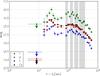 |
Fig. 1 Light curves in V (bottom), R, I (top) and the clear filter as recorded by the RAPTOR-T telescope. The magnitudes have not been corrected for the Galactic foreground extinction. The four epochs at which the UVES spectra were taken are indicated with the grey vertical bands. |
Log of RAPTOR-T observations.
GRB 080310 triggered the Burst Alert Telescope (BAT) onboard the Swift satellite (Cummings et al. 2008) at 08:37:58.65 UT on March 10, 2008. The RAPTOR-T telescope array began observing the BAT position within 10.7 s after receiving the GCN alert, i.e. 32.4 s after trigger time. RAPTOR-T consists of four co-aligned 0.4-m telescopes on a single fast-slewing mount and provides simultaneous images in four photometric bands (V, R, I and clear). The system, owned and operated by the Los Alamos National Laboratory (LANL), is located at the Fenton Hill Observatory at an altitude of 2500 m in the Jemez Mountains of northern New Mexico. The RAPTOR-T response sequence consists of 9, 20 and 170 exposures lasting, correspondingly, 5, 10 and 30 s each and separated by 5-s intervals for readout. Approximately 25% of individual frames were rejected due to intermittent glitches in telescope tracking.
Aperture photometry was performed on co-added images using the Sextractor package (Bertin & Arnouts 1996) with object coordinates fixed at the values measured on the reference image where the GRB is detected at a high signal-to-noise ratio (S/N) in all four channels. Instrumental light curves were then transformed to standard Johnson magnitudes using Sloan Digital Sky Survey (SDSS) photometry of stars in the vicinity of the burst (Cool et al. 2008) and equations of Lupton (2005)2. The results are listed in Table 1 and plotted in Fig. 1.
No optical emission was detected during the first two minutes after the burst, down to a limiting magnitude of R ~ 18.9 (3σ). The GRB is clearly detected in all subsequent co-adds starting at 133 s after the trigger. Following a rapid increase in brightness to a peak value at R ≃ 16.6 mag, the optical emission fluctuates by a few tenths of a magnitude and begins a slow decline after ~30 min. While the BAT light curve still shows a detectable gamma-ray emission between 150 and 320 s after the trigger (see Littlejohns et al. 2012), the optical emission over this time interval appears uncorrelated with the gamma rays. The optical light curves from RAPTOR-T show no significant colour evolution. We determined the spectral slope β (with Fν ∝ νβ) as a function of time, by first correcting the VRI magnitudes for the Galactic foreground extinction of EB − V = 0.045 (Schlegel et al. 1998), and then fitting them at each epoch. The resulting slope values do not show any trend in time, and cluster around the value β = −1.0, with a standard deviation of 0.4 and an error in the mean of 0.07.
The RAPTOR-T measurements are generally consistent with those reported in Littlejohns et al. (2012). The RAPTOR V- and R-band magnitude limits (3σ), at a mid-exposure time of 84 s after the burst, correspond to FV < 136 μJy and FR < 78 μJy, respectively. This V-band limit is in agreement with the Swift V-band measurement of FV = 247 ± 140 μJy at the same epoch, but our R-band limit is well below (almost a factor of three) the prompt-emission fit featured in Fig. 10 of Littlejohns et al. (2012). Instead, it is fully consistent with the alternative afterglow fit shown in their Fig. 8.
3. Modelling the absorption-line variability
In Paper I, we presented Voigt profile fits to the absorption lines detected in the GRB 080310 spectra, using four different velocity components. Since these are very close in velocity (<60 km s-1), it is difficult to ascertain that they are indeed correctly separated in the Voigt profile fit, even though a strong case can be made that components “b” and “c+d” probably are. Moreover, the decomposition is not unique, as additional components may be present that are hidden in the profile. An added complication is that it is unclear which fraction of the H i column density belongs to which velocity component; this is important for the modelling when ionizing radiation is included. Inspection of the Fe ii and Fe iii column density evolution of the separate components indicates a generally similar behaviour, which suggests that the components are at a comparable distance. Preliminary modelling of the separate velocity components “b” and “c+d” indeed results in distances that are the same within the error margins. For these reasons, we have focused on modelling the total column densities (listed in the last column of Table 3 in Paper I) rather than those of the individual components.
3.1. Photo-excitation
Since the absorption-line variability observed in a handful of GRBs can be generally well
described by excitation of the host-galaxy ISM by afterglow UV photons, we first set out
to model the GRB 080310 observed column density evolution as reported in Paper I with
photo-excitation alone. The excitation fitting procedure applied here is similar to that
described in Vreeswijk et al. (2007), which was
also applied by Ledoux et al. (2009) and
independently by D’Elia et al. (2009a,b, 2010). There
are, however, two major differences. First, we include the correct excitation flux (see
the erratum published by Vreeswijk et al. 2011),
resulting in a distance decrease of  with respect to the old excitation calculation. Second, instead of calculating the
excitation at line centre only, we effectively integrate over the full line profile to
obtain the actual flux that is entering a particular layer. This second change leads to a
modest increase in the distance estimate of about 10%. The details of the excitation
implementation are described in Appendix A.
with respect to the old excitation calculation. Second, instead of calculating the
excitation at line centre only, we effectively integrate over the full line profile to
obtain the actual flux that is entering a particular layer. This second change leads to a
modest increase in the distance estimate of about 10%. The details of the excitation
implementation are described in Appendix A.
For the Fe ii ion, we use the transition probabilities of the 371-level model
atom as collected by Verner (1999), including the
63 lower even-parity and 227 higher odd-parity levels. The transitions between even-parity
levels are forbidden and have low transition probabilities, while the transitions between
even- and odd-parity levels are electric dipole, i.e. allowed transitions. The resonance
and fine-structure lines observed in the spectra of GRB 080310 and other GRBs correspond
to this latter group. This 371-level model Fe ii atom is supplemented with
transitions taken from the Kurucz database (Kurucz
& Bell 1995)3. For Fe iii,
we apply two different model atoms. From the one calculated by Raassen &
Uylings4, we include 59 even-parity and 214
odd-parity levels. The alternative model, which we find to provide a slightly better fit,
combines the A-values for the forbidden transitions between the lowest 34
levels calculated by Bautista et al. (2010) with the
allowed transitions from Deb & Hibbert
(2009). In Paper I, we also present measurements and upper limits of the
excited-level column densities of Si ii and C ii, which we include in
our fit as well. The transition probabilities of both these ions are taken from Morton (2003) if present therein, otherwise they are
taken from the National Institute of Standards and Technology (NIST) atomic spectra
database5 (for the Si ii and C ii
transition probabilities and their references, see Kelleher & Podobedova 2008; Wiese
& Fuhr 2007). We note that Bautista et al.
(2009) have also calculated the A-values of several
Si ii transitions; we find that using those values instead of the NIST ones
leads to a very similar amount of Si ii excitation. For Si ii, we
include the ground level,  , its
corresponding fine-structure level
, its
corresponding fine-structure level  and 19
higher even-parity levels. For C ii, we include the lowest two levels
( and
) and 28
higher levels. For both these ions, the energy level of the third odd-parity level is
larger than the lower even-parity levels, so the number of atoms populating the other
Si ii and C ii odd-parity levels is expected to be negligible.
Finally, for Cr ii, we include the lowest 74 even-parity levels and nearly 400
odd-parity levels, adopting the A-values of the forbidden transitions
from Quinet (1997) and those of the allowed
transitions from Kurucz & Bell (1995). For
all ions, we made sure that the oscillator strengths (or equivalently, the transition
probabilities) of the relevant electric dipole transitions that are used to obtain the ion
column densities from the data through Voigt profile fitting (see Paper I) are the same as
used in the excitation modelling.
and 19
higher even-parity levels. For C ii, we include the lowest two levels
( and
) and 28
higher levels. For both these ions, the energy level of the third odd-parity level is
larger than the lower even-parity levels, so the number of atoms populating the other
Si ii and C ii odd-parity levels is expected to be negligible.
Finally, for Cr ii, we include the lowest 74 even-parity levels and nearly 400
odd-parity levels, adopting the A-values of the forbidden transitions
from Quinet (1997) and those of the allowed
transitions from Kurucz & Bell (1995). For
all ions, we made sure that the oscillator strengths (or equivalently, the transition
probabilities) of the relevant electric dipole transitions that are used to obtain the ion
column densities from the data through Voigt profile fitting (see Paper I) are the same as
used in the excitation modelling.
3.1.1. Excitation modelling input flux spectrum
The afterglow UV flux at the GRB-facing side of the absorbing cloud is obtained by converting the R-band brightness as observed by the RAPTOR-T telescope (see Sect. 2) to the host-galaxy redshift at a particular distance (a fit parameter) from the GRB. This conversion includes a correction for both the Galactic extinction of AR = 0.12 mag (Schlegel et al. 1998), and any possible extinction in the host galaxy. The latter was found to be of type Small Magellanic Cloud (SMC), with an estimated V-band extinction (in the host-galaxy rest frame) of AV = 0.19 ± 0.05 mag (Kann et al. 2010); we adopt this value for our main fits and assume that the dust responsible for this extinction is located within the absorbing cloud. The R-band light curve is interpolated in log space to obtain the brightness at any given time to be used in the model calculations. To determine the flux at different frequencies, we initially adopt a value for the spectral slope of β = −0.75 (the same as that adopted by Littlejohns et al. 2012). We note that β represents the intrinsic spectral slope, i.e. before it is affected by the host-galaxy extinction (if non-zero). The combination of this slope with an extinction of AV = 0.19 mag agrees well with the observed spectral slope β = −1, obtained from fitting the RAPTOR VRI data. Apart from this default slope-extinction setting, we also performed fits with zero host-galaxy extinction and the slope set to the observed value of β = −1. Since the afterglow flux in the X-ray regime is not relevant for excitation, we do not consider the X-ray flux.
3.1.2. Excitation-only fit result
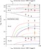 |
Fig. 2 Photo-excitation modelling of the observed (total) column densities as a function
of time, as measured in Paper I (see their Table 3), for C ii,
Si ii, Fe ii and Fe iii. The open circles are
detections, while the open triangles indicate upper or lower limits
(3σ). The different colours denote the different ion levels:
black for the ground state and red-green-maroon-orange for the first four excited
levels, while the Fe ii |
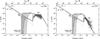 |
Fig. 3 Adopted input flux spectrum that is arriving at the GRB-facing side of the observed cloud (in observed flux units) depicted at two different epochs: tobs = 225 s on the left and tobs = 672 s on the right. The solid line shows the default input spectrum with a spectral slope of β = −0.75 up to 0.3 keV, above which the X-ray flux (at 1.73 keV) and spectral slope is adopted. The RAPTOR VRI and Swift XRT observations corresponding to these epochs are overplotted with open squares. The long-dashed line shows the default input spectrum modified by an extinction of AV = 0.19 mag; since this extinction is placed inside the observed cloud, it is not observable at the front of the cloud. The dotted line shows the input spectrum assuming a spectral slope of β = −1, combined with no extinction. The dashed line between the observed optical and X-ray regimes shows our approximation to the Littlejohns model flux. The energy and flux limits of this figure are the same as those in Fig. 9 of Littlejohns et al. (2012) for easy comparison. The hashed regions show the flux decrease due to a foreground cloud with H i column density log N(H i) = 18.9 for the default input flux model (horizontal lines) and log N(H i) = 20.3 for the alternative Littlejohns input spectrum (vertical lines); see Sect. 4 and Table 3 for more details. The ionization edges of He i at 24 eV/(1+z) and He ii at 54 eV/(1+z) can be spotted. We note that the spectral region between the Lyman limit and the X-ray data is not constrained by imaging observations. |
The column density evolution of Fe ii, Fe iii, Si ii and
C ii (both ground-state and excited levels) is fit with an excitation-only
model, which includes the following fit parameters: 1) the GRB to cloud distance, i.e.
the distance from the GRB to the front of the cloud, facing the GRB6, 2) the linear cloud size, 3) the pre-burst Fe ii,
Fe iii, Si ii and C ii column densities and 4) the Doppler
parameter describing the velocity distribution of the atoms. The resulting fit, shown in
Fig. 2, describes the observed column densities
quite poorly, with a large reduced chi-square value
( ).
One of the main reasons for the poor fit is that all observed levels of Fe ii
are decreasing with time, which cannot be accommodated with excitation alone. We note
that, based on the atomic transition probabilities between the different levels, it is
not possible for a large fraction of the pre-burst Fe ii atoms to be excited to
levels above those of the ground term (6D). Moreover, transitions from these
higher levels are not observed (see Paper I); e.g. see the
Fe ii
).
One of the main reasons for the poor fit is that all observed levels of Fe ii
are decreasing with time, which cannot be accommodated with excitation alone. We note
that, based on the atomic transition probabilities between the different levels, it is
not possible for a large fraction of the pre-burst Fe ii atoms to be excited to
levels above those of the ground term (6D). Moreover, transitions from these
higher levels are not observed (see Paper I); e.g. see the
Fe ii level upper
limits (indicated by the blue triangles) in Fig. 2.
Another feature that is very difficult to explain with excitation alone is the very
large observed fraction of Fe iii atoms in the excited
level upper
limits (indicated by the blue triangles) in Fig. 2.
Another feature that is very difficult to explain with excitation alone is the very
large observed fraction of Fe iii atoms in the excited
 level of
the order of 10% (see the blue level in the bottom panel of Fig. 2). This level is severely underestimated by the model fit, despite
the best-fit cloud distance being lower than 50 pc. For these reasons, we can
confidently reject the hypothesis that excitation alone is responsible for the observed
column density evolution along the GRB 080310 sightline.
level of
the order of 10% (see the blue level in the bottom panel of Fig. 2). This level is severely underestimated by the model fit, despite
the best-fit cloud distance being lower than 50 pc. For these reasons, we can
confidently reject the hypothesis that excitation alone is responsible for the observed
column density evolution along the GRB 080310 sightline.
3.2. Inclusion of photo-ionization
Excitation of an ion in a particular ionization state does not change the total number of
ions in that state. However, the observed Fe ii column densities all clearly
decrease in time, including the ground state whose variability is generally not detected.
This suggests that Fe ii may be increasingly ionized (by the GRB afterglow) to
higher ionization states such as Fe iii (see Paper I). This hypothesis is
supported by the detection of transitions of Fe iii, involving both the ground
state and the excited
level; this latter level has never been observed before along a GRB sightline. Moreover,
in Paper I we find that the Fe iii level
population is clearly increasing with time. Given this observational evidence for
photo-ionization and our finding above that photo-excitation alone cannot reproduce the
column density evolution observed, we have included photo-ionization in our model
calculations.
3.2.1. Modelling input flux spectrum: inclusion of X-rays
With the inclusion of photo-ionization, we need to consider both the UV and X-ray afterglow radiation. X-ray photons photo-ionize species such as Fe ii, Si ii and Fe iii mainly via the ejection of inner-shell electrons. Since the X-ray flux for GRB 080310 is not a simple extrapolation of the optical/UV flux with the optical spectral slope (see Littlejohns et al. 2012), we include the X-ray light curve as measured by the Swift XRT. We retrieved the 0.3−10 keV XRT afterglow light curve in count rate from the Swift repository (Evans et al. 2009) and separated it in eight different time intervals (0–141, 141–185, 185–269, 269−393, 393−545, 545–615, 615–796, 796–7261 s after the trigger) in order to limit the possible X-ray spectral evolution in each single isolated light curve track. We then extracted the spectrum from the repository for each time interval and converted the count rate light curve to flux density accordingly. The monochromatic flux at 1.73 keV (logarithmic average of the X-ray band) was calculated assuming the correspondent spectral slopes for each window. This X-ray light curve replaces the R-band extrapolation in the regime above 0.3 keV (in the observer’s frame, corresponding to 1.0 keV in the host galaxy rest frame). In the region 0.3−10 keV, we adopt the spectral slopes determined for the different time intervals, and beyond 10 keV we adopt a spectral slope of β = −2 at all times (see Littlejohns et al. 2012). The X-ray spectra and assumed spectral slopes are shown for two time intervals (185–269 and 615–796 s) in Fig. 3.
We also performed fits with an alternative to the input flux spectrum described above. This alternative is motivated by modelling of the GRB 080310 afterglow by Littlejohns et al. (2012), which suggests that the early-time flux (up to about 1800 s in the observer’s frame) between roughly 3 eV and 300 eV is much higher than the β = −0.75 (or β = −1) extrapolation from the optical (see Fig. 9 of Littlejohns et al. 2012). We note that this regime has no observations that are able to constrain the proposed model. The Littlejohns model flux is approximated by interpolation of the RAPTOR optical and Swift X-ray light curves between 3000 Å (3.6 eV) and 300 eV (both in the observer’s frame). Below and above this region, the flux used is the same as the original input flux spectrum described above. In Fig. 3, we show the default input spectrum (solid line) and the Littlejohns alternative (dashed line) at two different epochs. In the modelling, the input spectrum is constructed by interpolation of the the RAPTOR R-band and Swift XRT light curves for each new time step.
3.2.2. Cross section of Fe II ionization to different levels of Fe III
Our programme incorporates well-known astrophysical processes (e.g. Osterbrock & Ferland 2006), and we refer the reader to Appendix A for a detailed description of how the photons excite and ionize the ions in the absorbing cloud. We stress that ionization is taken into account for all relevant ions, i.e. H i, He i, He ii, Fe ii, Fe iii, Si ii, C ii and Cr ii, and that we properly consider the fraction of Fe ii that will be ionized to Fe iii (rather than to higher ionization states), as calculated by Kaastra & Mewe (1993) for the different ion shells. Excitation is included for all ions, except for hydrogen and helium. One very important non-standard aspect, the calculation of the cross section of Fe ii ionization to different (excited) levels of Fe iii, is discussed here.
When Fe ii is ionized to Fe iii, the Fe iii ion will not necessarily be in its ground state, at least not immediately. We calculated the photo-ionization cross section from Fe ii to specific levels of Fe iii using two different codes: the suite of programmes developed by Cowan (1981) and the Flexible Atomic Code (FAC) developed by Gu (2003, 2004). The Cowan code is a self-consistent Hartree-Fock model with relativistic corrections. The FAC package is also a self-consistent programme, which models the wave functions to self-consistency by including the electron screening. Relativistic effects are taken into account by means of the Dirac Coulomb Hamiltonian.
The lowest configurations in Fe ii, 3d7 and 3d64s,
strongly overlap, having 3d6(5D)4s
 as their
ground state. However, the 6D magnetic J-sublevels are just
slightly higher in energy and are all populated (see Paper I). Since no absorption
features from higher lying levels in Fe ii have been observed (see Table 3 of
Paper I), we focused on ionization from the low-lying 6D levels. The
character of the configuration that the ground state belongs to (3d64s)
results in a photo-ionization process that is both complex and interesting. There are
several channels to ionization from the ground configuration, including (a)
3d64s → 3d6 by ionizing the outer 4s-electron to the
p-continuum by means of a photon absorption, and (b) 3d64s →
3d54s by ionizing the 3d-electron to the p- or f-continuum by means of a
photon absorption.
as their
ground state. However, the 6D magnetic J-sublevels are just
slightly higher in energy and are all populated (see Paper I). Since no absorption
features from higher lying levels in Fe ii have been observed (see Table 3 of
Paper I), we focused on ionization from the low-lying 6D levels. The
character of the configuration that the ground state belongs to (3d64s)
results in a photo-ionization process that is both complex and interesting. There are
several channels to ionization from the ground configuration, including (a)
3d64s → 3d6 by ionizing the outer 4s-electron to the
p-continuum by means of a photon absorption, and (b) 3d64s →
3d54s by ionizing the 3d-electron to the p- or f-continuum by means of a
photon absorption.
The result of (a) is the population of the Fe iii 3d65D states, while (b) ends up in the Fe iii 3d5(6S)4s 7S or 5S states. In Fe iii, there is quite an energy difference (3.7 eV) between 3d65D and 3d5(6S)4s7S. The fact that absorption features are observed arising from these states and not from states in between indicates that the dominant role is played by photo-ionization rather than by collisional excitation.
In the approach using the Cowan Code, the even configurations 3d7 and
3d64s and the odd continuum states 3d6ϵp and
3d54s ϵp and ϵf were applied. In case of
FAC, the Fe ii 3d64s and 3d7 as well as the
Fe iii 3d54s and 3d6 configurations were introduced in
the modelling. Comparison of the results from the Cowan and FAC programmes shows a very
good general agreement. Table 2 lists the
calculated cross sections for the relevant levels of Fe iii and the
corresponding fraction of Fe ii ionizations that populate that particular
Fe iii level. These numbers are used directly in our modelling programme7. We find that only a small fraction (9%) will
directly populate the Fe iii ground term, while 31% of the new Fe iii
ions will in fact populate the level. The
majority (57%) will populate the levels of the 3d5(4G)4s
5G term. However, these levels will quickly decay to the
3d65D ground term. Figure 4
shows a partial energy diagram of some relevant terms of Fe iii. While many
more terms exist, we do not depict them in the interest of clarity. For each relevant
transition (indicated with the dotted line), we list the logarithm of the transition
probability. For the strongest transition between the 3d54s 5G and
3d65D terms, for example, this is
A = 10+2.0 s-1. The reciprocal of this number
provides the time in seconds in which the ions in the upper level would decay to the
lower level in the absence of radiation.
Cross sections for ionization of ground-term Fe ii ions to different excited levels of Fe iii, as calculated with the FAC and Cowan codes.
Column-density evolution modelling fit results.
3.2.3. Comparison with ionization calculations in the literature
As a consistency check, we compared the amount of ionization computed in our programme with calculations in the literature. Since our ionization model does not take into account recombination8, while most calculations in the literature do, the comparison options are limited to GRB ionization studies. Examples of these are the studies of Perna & Lazzati (2002), Perna et al. (2003) and Draine & Hao (2002), in which not only the ionization induced by the GRB is calculated, but also the accompanying destruction of dust and dissociation of H2. Since our programme does not include dust destruction, a comparison with these calculations is difficult. However, we were able to compare our programme with the H, He and N photo-ionization calculations by Prochaska et al. (2008) and find consistent results. We use their Eq. (8) for the GRB 050730 afterglow luminosity over the same time span tobs = 10–1000 s and adopt their set-up with nH = 10 cm-3, a nitrogen-to-hydrogen abundance ratio of 10-6 (roughly 0.01 solar metallicity), and assume that before the GRB all the ions are in the singly ionized state. We then switch on the GRB 050730 afterglow and follow the progressive ionization of N ii to higher ionization states, finding that after 1000 s, the N v column density remaining is log N(N v) = 13.8, compared to their log N(N v) = 14. Also, the ionization structure at tobs = 1000 s computed by our programme is very similar to that depicted in their Fig. 3.
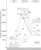 |
Fig. 4 Partial energy level (or Grotrian) diagram for the relevant lower terms of the three lowest configurations of Fe iii: 3d6, 3d54s and 3d54p (indicated at the top). The horizontal solid lines depict the energy levels, labelled with the term and J-value. Selected transitions are shown with dotted lines between levels. For each transition, we list the logarithm of the transition probability (or Einstein A-coefficient, in (s-1)) of the strongest transition between the terms, adopting the Raassen & Uylings values (see Sect. 3.1). |
3.2.4. χ2 minimization and fit parameters
The model column densities computed by our programme, as detailed in Appendix A, are fit to the observed GRB 080310 column densities at their respective epochs. We use the Fortran 90 version of the MINPACK lmdif χ2 minimization routine (Moré et al. 1980, 1984), which is based on the Levenberg-Marquardt method. We have made this programme parallel with OpenMP, so that it can be run faster on a shared-memory computer cluster. The formal errors of the fit parameters are estimated by computing the co-variance matrix and taking the square root of the diagonal elements.
The fit parameters are the same as those used in the excitation-only case described at the end of Sect. 3.1: the GRB to cloud distance (i.e. the distance from the GRB to the GRB-facing side of the cloud), the cloud size, the Doppler parameter b and a pre-burst column density for each ion included in the fit. We again initially fix the spectral slope to β = −0.75 (see Littlejohns et al. 2012), in combination with a host-galaxy extinction of AV = 0.19 mag (Kann et al. 2010), but also experiment with the combination β = −1.0 and zero extinction. The ions included are Fe ii, Fe iii, Si ii, C ii and Cr ii (apart from H i, He i and He ii, see below), i.e. all low-ionization species with a total column density measurement at one or more epochs as reported in Table 3 of Paper I. For all of these we include excitation.
As discussed in Paper I, the velocity profiles of Fe ii and Fe iii are markedly different from those of Si ii and C ii. The former are dominated by component “b” at −20 km s-1 from the systematic velocity and with a Doppler broadening parameter value of b = 13 km s-1. However, a considerable column density is also contained in the other components “a”, “c” and “d”, leading to an overall broad velocity structure for Fe ii and Fe iii. In contrast, the vast majority of the Si ii and C ii column densities are located in the narrow “c” component at the systematic velocity, with b = 7 km s-1. For this reason, we split the Doppler broadening fit parameter into two: one for Fe ii and Fe iii (bFe II, Fe III) and one for Si ii and C ii (bSi II, C II).
In Paper I, we also constrained log N(H i) to 18.7 at two different epochs. This H i column density is an important quantity because if sufficiently large, it can effectively shield the low-ionization species (such as Fe ii and Si ii) from the ionizing photons. Besides H i, we also include He i and He ii, which are also important for shielding, albeit at higher photon energies (starting from 24 eV). These helium ions do not require additional fit parameters, as we fix the He i column density at the solar abundance value (i.e. 8.5% of N(H i), Asplund et al. 2009) and set the pre-burst He ii column density to zero. We note that the inclusion of a significantly larger amount of He i (a possibility if there is a large column density of pre-burst ionized hydrogen) does not affect our results. If the He i abundance is included in the fit as a free parameter, the best-fit value is consistent with the adopted value: [He i/H i] = (12 ± 17)%.
4. Results
The resulting fit to the total column densities is shown in Fig. 5. The solid (dotted) lines correspond to the best-fitting model, assuming
the default (Littlejohns) input flux discussed in Sect. 3.2. The goodness-of-fit and best-fit parameter values are listed in the first
column of Table 3. The model fit in which the
Littlejohns input flux is adopted is very poor, with  and we
therefore discard it without listing the unreliable best-fit parameter values in Table 3. The quality of the model fit that assumes the default
input flux is reasonable, with
and we
therefore discard it without listing the unreliable best-fit parameter values in Table 3. The quality of the model fit that assumes the default
input flux is reasonable, with  . This
rather high value for the reduced chi-square seems to be mainly caused by the model
underpredicting the observed population of the Fe ii excited levels. Assuming a
negligible host-galaxy extinction (AV = 0 mag) combined with the
observed spectral slope of β = −1 leads to a slightly improved fit with a
chi-square value of
. This
rather high value for the reduced chi-square seems to be mainly caused by the model
underpredicting the observed population of the Fe ii excited levels. Assuming a
negligible host-galaxy extinction (AV = 0 mag) combined with the
observed spectral slope of β = −1 leads to a slightly improved fit with a
chi-square value of  , but
with resulting best-fit values consistent within the errors of the default fit (with
β = −0.75 and AV = 0.19 mag).
, but
with resulting best-fit values consistent within the errors of the default fit (with
β = −0.75 and AV = 0.19 mag).
Table 3 shows that the best-fit Si ii and C ii Doppler broadening parameter is very low: bSi II,C II = 2.1 ± 0.7 km s-1. As we discussed in the previous section, the observed b-parameter value is low as well: bSi II,C II = 7 km s-1. To investigate this modest discrepancy further, we also ran a model in which only H i, He i, Si ii and C ii are included, i.e. without Fe ii, Fe iii and Cr ii and with the b-parameter fixed to the observed value of b = 7 km s-1. Although the resulting distance to the GRB-facing side of the cloud is very small, less than 50 pc, the cloud size becomes more than a kiloparsec, i.e. the average distance is quite large. Forcing the cloud to be very compact, with a cloud size fixed at 1 pc, yields a best-fit distance, both without and with the Littlejohns input flux, of roughly 600 pc. These results indicate that the majority of Si ii and C ii ions might be at a different location (further away from the GRB) or spread out over a larger region than the bulk of the Fe ii and Fe iii ions. This is supported by the very different velocity profiles that these ions display (see Paper I). However, for other GRB sightlines for which a cloud distance has been determined independently for Fe ii and Si ii excitation (e.g. D’Elia et al. 2010, 2011), the best-fit distances are consistent. This suggests that, as one would expect, the Fe ii and Si ii atoms are probably located at comparable distances from the GRB.
Since the Fe ii excited levels are underpredicted by the model, we attempted to
place an additional cloud along the line of sight, in between the GRB and the observed
absorber or cloud. If the additional cloud were sufficiently close to the burst, it would
become completely ionized during the first few tens of minutes (in the observer’s frame) of
the arrival of the GRB radiation and would not reveal itself in the observations. But at the
same time, it would partially shield the observed cloud from ionizing radiation released
during the first minutes after the GRB, allowing the observed cloud to be closer to the
burst and thus increasing the amount of excitation. This scenario could only work if the two
clouds have a velocity offset (10–20 km s-1 is sufficient and not unlikely), to
prevent the observed cloud from being in the absorption-line shadow of the foreground cloud.
The fit with such an additional cloud is shown in Fig. 6, again with the solid (dotted) curves corresponding to the model fit adopting
the default (Littlejohns) input flux and the best-fit parameter values are listed in the
second and third columns of Table 3. The addition of
such a foreground cloud results in a lower value for the chi-square
( ,
assuming the default input flux), but at the expense of three additional fit parameters: the
distance, size and column density of the foreground cloud (see Table 3). An F-test suggests that the fit improvement introduced by the
foreground cloud is significant, providing
,
assuming the default input flux), but at the expense of three additional fit parameters: the
distance, size and column density of the foreground cloud (see Table 3). An F-test suggests that the fit improvement introduced by the
foreground cloud is significant, providing 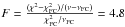 (where ν is
the number of degrees of freedom) and a null probability of
P < 0.005; i.e. there is less than 0.5% chance
that such an improvement is random.
(where ν is
the number of degrees of freedom) and a null probability of
P < 0.005; i.e. there is less than 0.5% chance
that such an improvement is random.
We also ran model fits with both a foreground cloud and adoption of the alternative
Littlejohns input flux. As described in Sect. 3.2, this
input flux is much higher (up to a factor of 10) than the default input flux between 0.3 eV
and 300 eV (see Littlejohns et al. 2012), leading to
much more ionizing radiation. As mentioned above, a model fit with the Littlejohns input
flux without an additional cloud describes the observed column density
evolution very poorly. However, an additional cloud with a neutral hydrogen column density
almost that of a damped Lyα (DLA) system at 10–20 pc from the GRB is
capable of absorbing most of the extra ionizing radiation, leading to a very reasonable fit
(with  ). The
best-fit parameter values for this model are listed in the third column of Table 3 and the resulting column density evolution is shown
with a dotted line in Fig. 6.
). The
best-fit parameter values for this model are listed in the third column of Table 3 and the resulting column density evolution is shown
with a dotted line in Fig. 6.
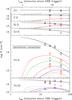 |
Fig. 5 Photo-excitation and -ionization modelling of the observed (total) column densities as a function of time, as measured by De Cia et al. (2012) (see Table 3 of Paper I), for H i, C ii, Si ii, Cr ii, Fe ii and Fe iii (from top to bottom panels). The solid and dotted lines correspond to the best-fitting model, assuming the default and the Littlejohns input flux, respectively. The different colours of the symbols and lines have the same meaning as in Fig. 2. Although overall the model provides a reasonable description of the column density evolution, the observed excited levels of Fe ii at epoch II are significantly underestimated. See the text and Table 3 for more details. |
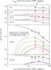 |
Fig. 6 Same as Fig. 5, but including a foreground cloud situated between the GRB and the observed absorber. The solid and dotted lines correspond to the best-fitting model, assuming the default and Littlejohns input flux, respectively. The foreground absorber is mostly ionized by the time of the second epoch UVES spectrum and can therefore escape a clear detection. See the text and Table 3 for more details. |
5. Discussion
The evolution of the Fe ii and Fe iii column densities observed at the
GRB 080310 redshift (see Paper I and Sects. 3.2 and
4), combined with our modelling, clearly shows that
ionization of Fe ii is taking place. A very strong argument in favour of ionization
and a vital ingredient for the modelling is that according to our calculations (see Sect.
3.2.2), a large fraction (31%) of Fe ii
ionizations will initially populate the
Fe iii level. Without
taking this effect into account, we found it impossible to explain the large fraction
(~10%) of Fe iii that is observed to be in this particular level (see Paper I).
This channel for producing a significant
Fe iii level
population may be relevant for other objects in which absorption lines from this level, the
UV34 triplet, are also observed, such as broad absorption line (BAL) quasars and
η Carinae. As it takes about 1000 s for the
Fe iii level
population to decay spontaneously down to the ground term, the Fe ii ionization
rate needs to be significant at this time scale for this process to be relevant. The UV48
triplet, at 2062, 2068 and 2079 Å, is sometimes detected in BAL quasars. The lower energy
level from which the UV48 triplet arises,  (see
Fig. 4), receives only a small fraction of the
Fe ii ions that are ionized to Fe iii (1%, see Table 2) and so these lines are expected to be much weaker than
the UV34 triplet. We checked for the presence of these UV48 absorption lines in the UVES
spectra of GRB 080310 and did not detect them. In the sample of unusual BAL quasars of Hall et al. (2002), the detection of the UV34 triplet is
much more common than UV48, which would be expected if ionization of Fe ii is the
dominant mode of populating the UV34 lower level. However, if the UV48 absorption is
stronger than that of UV34, as in SDSS 2215–0045 (Hall et
al. 2002; Vivek et al. 2012), the
above-mentioned Fe iii excited-level population scenario, which works well for
GRB 080310, does not provide a viable explanation.
(see
Fig. 4), receives only a small fraction of the
Fe ii ions that are ionized to Fe iii (1%, see Table 2) and so these lines are expected to be much weaker than
the UV34 triplet. We checked for the presence of these UV48 absorption lines in the UVES
spectra of GRB 080310 and did not detect them. In the sample of unusual BAL quasars of Hall et al. (2002), the detection of the UV34 triplet is
much more common than UV48, which would be expected if ionization of Fe ii is the
dominant mode of populating the UV34 lower level. However, if the UV48 absorption is
stronger than that of UV34, as in SDSS 2215–0045 (Hall et
al. 2002; Vivek et al. 2012), the
above-mentioned Fe iii excited-level population scenario, which works well for
GRB 080310, does not provide a viable explanation.
Time variation of H i and metal-column densities due to the ongoing ionization by the GRB and afterglow radiation has been predicted (e.g. Perna & Loeb 1998), but has never been convincingly detected before (see Thöne et al. 2011). This applies not only to neutral-medium ions such as H i and Fe ii, but also to high-ionization species as C iv and N v (Fox et al. 2008; Prochaska et al. 2008). The reason that ongoing photo-ionization is observed for GRB 080310 is not that the observed neutral material along the GRB 080310 sightline is much closer to the GRB than in other cases. We find a distance range of 200–400 pc (depending on the adopted input flux and the inclusion or not of a foreground cloud, see Sect. 4 and below), while other GRBs for which only excitation was detected have distance estimates as low as 50 pc (D’Elia et al. 2011). In Table 4, we have collected the GRB-cloud distance estimates from the literature, allowing for a direct comparison with the distance estimate for GRB 080310. We note that, in the absence of a foreground cloud, a lower limit of about 100 pc can be placed on the GRB-absorber distance by just considering the non-variation in the H i column density between 21 and 50 min post-burst. If the absorber had been much closer, we would have detected a significant H i column density change.
GRB absorber distances, as of April 2012.
We investigated whether the very low H i column density or super-solar iron
abundance along the GRB 080310 sightline is the reason for the unique detection of ongoing
ionization. We did so by running models with most parameters fixed to the best-fitting model
(with  in
Table 3), but varying the H i column density
and iron abundance to see how these affect the number of ions detected in the
Fe iii level. As we
have shown above, a significant population of this excited level is a clear sign of ongoing
ionization of Fe ii. Table 5 shows the
expected peak Fe iii column density
as a function of different H i column densities (rows) and iron abundances
(columns). In the column with fixed
NFeII,FeIII, we fixed the pre-burst
Fe ii and Fe iii column densities at their best-fit values (middle
column) of Table 3 for the four different
H i column densities, while in the last two columns, all the iron was assumed to
be in the singly ionized state before the GRB exploded; we note that this latter assumption
is only valid at higher H i column densities
(log N(H i) ~ >20).
in
Table 3), but varying the H i column density
and iron abundance to see how these affect the number of ions detected in the
Fe iii level. As we
have shown above, a significant population of this excited level is a clear sign of ongoing
ionization of Fe ii. Table 5 shows the
expected peak Fe iii column density
as a function of different H i column densities (rows) and iron abundances
(columns). In the column with fixed
NFeII,FeIII, we fixed the pre-burst
Fe ii and Fe iii column densities at their best-fit values (middle
column) of Table 3 for the four different
H i column densities, while in the last two columns, all the iron was assumed to
be in the singly ionized state before the GRB exploded; we note that this latter assumption
is only valid at higher H i column densities
(log N(H i) ~ >20).
Maximum Fe iii column
density reached as a function of the assumed H i column and iron abundance in
the GRB 080310 absorber.
Considering log  to be the approximate lower
limit for a clear detection of this level in the UVES spectra, Table 5 shows that increasing the H i column density by a factor of
about 100 or more, while fixing the Fe ii and Fe iii column densities at
the best-fit values of Table 3, would have resulted
in a non-detection of the Fe iii excited level. This is due to the increased
shielding of the low-ionization metals from the ionizing radiation by the H i and
He i atoms. However, when fixing the abundance at the observed value for iron
along the GRB 080310 sightline ([Fe/H] = +0.2, see Paper I), the Fe iii excited
level is detected at any H i column density. At a more typical iron abundance for
GRB sightlines, [Fe/H] = −1.0, the Fe iii UV34 triplet is detectable only at
the higher H i column density end. We note that a column density of
log N(H i) = 21.6 at 0.1 Z⊙
implies a considerable Fe ii column (log
N(Fe ii) = 16.1) and this increases by at least a factor of ten
when assuming [Fe/H] = +0.2. At such large Fe ii columns, dust is not unlikely
to be present. The presence of dust would complicate the UV34 triplet detection at high
H i columns. Dust obscuration would not only decrease the amount of ionization
taking place, but would also make it more difficult to detect a bright afterglow, which is
required to secure high-quality spectra. Therefore, the reason for the unique detection of
the Fe iii UV34 triplet in the GRB 080310 spectra appears to be a combination of
the super-solar iron abundance and the low H i column along this sightline. This
ensures the presence of a sufficient amount of iron, while at the same time avoiding too
much H i and He i shielding and dust obscuration.
to be the approximate lower
limit for a clear detection of this level in the UVES spectra, Table 5 shows that increasing the H i column density by a factor of
about 100 or more, while fixing the Fe ii and Fe iii column densities at
the best-fit values of Table 3, would have resulted
in a non-detection of the Fe iii excited level. This is due to the increased
shielding of the low-ionization metals from the ionizing radiation by the H i and
He i atoms. However, when fixing the abundance at the observed value for iron
along the GRB 080310 sightline ([Fe/H] = +0.2, see Paper I), the Fe iii excited
level is detected at any H i column density. At a more typical iron abundance for
GRB sightlines, [Fe/H] = −1.0, the Fe iii UV34 triplet is detectable only at
the higher H i column density end. We note that a column density of
log N(H i) = 21.6 at 0.1 Z⊙
implies a considerable Fe ii column (log
N(Fe ii) = 16.1) and this increases by at least a factor of ten
when assuming [Fe/H] = +0.2. At such large Fe ii columns, dust is not unlikely
to be present. The presence of dust would complicate the UV34 triplet detection at high
H i columns. Dust obscuration would not only decrease the amount of ionization
taking place, but would also make it more difficult to detect a bright afterglow, which is
required to secure high-quality spectra. Therefore, the reason for the unique detection of
the Fe iii UV34 triplet in the GRB 080310 spectra appears to be a combination of
the super-solar iron abundance and the low H i column along this sightline. This
ensures the presence of a sufficient amount of iron, while at the same time avoiding too
much H i and He i shielding and dust obscuration.
If the detection of Fe ii ionization is indeed due to a combination of the super-solar iron abundance and the low H i column density along the GRB 080310 sightline in the host, then the (non-)detection of the Fe iii UV34 triplet can be used to put constraints on the H i column density along a GRB sightline with an Fe ii detection in case it cannot be inferred from the spectrum. The latter is the case at z ≲ 2, when Lyα is not redshifted enough to be included in the optical wavelength range of spectrographs on ground-based telescopes. The strength of the Fe iii UV34 triplet, however, depends on various quantities besides the iron abundance and H i column, such as the GRB-absorber distance, the afterglow peak luminosity and brightness evolution and the time at which the spectra are taken. It is therefore difficult to provide a simple scaling relation between the H i column, iron abundance and UV34 triplet strength.
But for GRBs for which most of the above quantities can be constrained through absorption-line photo-excitation modelling, it is possible to determine a lower limit on the H i column density from the Fe iii UV34 triplet non-detection. As our team has already performed such modelling on GRB 060418 (at z = 1.490, Vreeswijk et al. 2007, 2011), we can readily determine this limit on H i for this sightline. The UV34 triplet is not detected in the GRB 060418 UVES spectra, with a 3σ upper limit on the rest-frame equivalent width (column density) of 0.03 Å (log N = 12.6). Modelling the excitation and ionization with our code, in which we vary the H i column density, we find that this UV34 detection limit corresponds to an H i column density limit of log N(H i) > 21.0. Using the total zinc column density measured for this sightline (log N(Zn ii) = 13.09 ± 0.01, Vreeswijk et al. 2007) and assuming that most of the zinc is in the singly ionized state, we found that the H i column density lower limit derived above implies an upper limit on the metallicity of [Zn/H] < −0.5. Determining these H i column-density and corresponding metallicity limits for the entire sample of Table 4 requires separate photo-excitation and -ionization modelling for each sightline, which is out of the scope of the current paper.
Our simplest model, in which the GRB afterglow is ionizing and exciting a cloud at a distance of about 360 pc, does not provide a satisfactory description of the observations. As can be seen in Fig. 5, the model underestimates the ground-term fine-structure level population. One potential reason for this lack of Fe ii excitation, or abundance of ionization, may be that additional neutral material is present between the GRB and the absorber responsible for the absorption features observed in the spectra. This additional absorber needs to be ionized by the time that the first couple of spectra are taken, as otherwise it would reveal itself in the observed spectra. Placing such an additional cloud closer to the GRB, with log N(H i) ~ 19 at a distance of tens of parsecs, improves the model fit significantly, as shown by the solid curves in Fig. 6. Also, in the case where the Littlejohns input flux is adopted (depicted by the dotted curves in Fig. 6), the model with a foreground cloud provides a very reasonable description of the observed column density evolution of the different ionic species. In this case, the foreground cloud is required to have a higher neutral hydrogen column density (log N(H i) = 20.3) and to be closer to the GRB (12 pc) in order to be able to absorb the additional ionizing photons in the Littlejohns input flux. The similar chi-squares for the additional-cloud model using the default and Littlejohns input fluxes do not allow us to favour one input flux over the other; however, in the model without an additional cloud, the default input flux is clearly favoured.
We tested if a log N(H i) = 20.3 cloud at 12 pc with an assumed metallicity of one tenth of solar and using the Littlejohns input flux would imply an observable N v variation (see Fox et al. 2008; Prochaska et al. 2008) in our spectra. In Paper I, we report a constant N v column density: log N(N v) = 14.10 ± 0.04 and log N(N v) = 14.05 ± 0.02 at epochs II and IV, respectively. In this test, we adopt a metallicity of one-tenth of the solar abundance and assume that all the nitrogen is singly ionized before the burst. We find that the N ii ions are very quickly ionized to higher ionization states. At six minutes after the burst (observer’s frame), the N v column density in the foreground cloud is already below log N(N v) = 13 and by the time of the first epoch spectrum (13 min after the burst), practically all the nitrogen has been ionized to states higher than N v. Also, if the foreground cloud is indeed ionized within about ten minutes of the arrival of the first GRB photons, it is very difficult to infer its presence in sightlines where only ongoing excitation is observed.
Although the introduction of an additional cloud is a rather ad hoc solution for improving the model fit of Fig. 5, the existence of an additional cloud in the vicinity of the burst is not unexpected, as GRBs are thought to occur in gas-rich massive-star forming regions (e.g. Prochaska et al. 2007). We note that the presence of such an additional cloud is consistent with the host-galaxy N(H)-equivalent X-ray absorption as inferred from the Swift XRT data (log N(H) = 21.7 ± 0.05 and log N(H) < 21 – assuming solar metallicity – for the time-averaged averaged windowed timing and photon counting modes, respectively, Evans et al. 2009). Thus, although the presence of a foreground cloud is plausible, we cannot exclude a different origin for the underestimate of the Fe ii excitation (or overestimate of ionization) in our default model fit.
6. Conclusions
We modelled the variability of the ionic column densities of various species (including
H i, He i, He ii, Fe ii, Fe iii,
Si ii, C ii and Cr ii) in the circumburst medium of GRB 080310
(reported in a companion paper by De Cia et al. 2012)
with a photo-excitation and -ionization radiative transfer code. The rest-frame
near-infrared to X-ray spectrum of the afterglow radiation and its time evolution, an
important input parameter in the modelling, is inferred by combining the RAPTOR-T
VRI light curves, also presented in this paper, and the X-ray light curve
as observed by Swift. We find that excitation alone, which has been
successfully applied to other GRBs, is not able to explain the GRB 080310 observations;
ionization is clearly required. The strongest evidence for ionization is presented by the
clear detection of the UV34 triplet of Fe iii from the lower level
. The large
fraction of Fe iii ions (10%) measured to be in this level can only be explained
through ionization of Fe ii; we calculate that 31% of all Fe ii ions that
end up as Fe iii will first populate this level.
This is the first conclusive evidence for the detection of time-variable photo-ionization
induced by a GRB afterglow.
Despite this evidence for photo-ionization, the distance between the GRB and the absorbing medium that we infer (200−400 pc) is very similar to that in other GRB sightlines for which such a distance estimate was possible. We find that the main reason for detecting time-variable ionization in this GRB and not in others is the super-solar iron abundance ([Fe/H] = +0.2) in combination with the low H i column density (log N(H i) = 18.7 ± 0.1) along this sightline.
The combined photo-excitation and -ionization modelling provides tentative evidence for the presence of an additional absorbing cloud, with log N(H i) ~ 19–20, at a distance of 10−50 pc from the GRB, even though this cloud is almost completely ionized by the afterglow within a few tens of minutes (in the observer’s frame) of the arrival of the GRB radiation. Future time-resolved high-resolution spectroscopic observations of low-H i GRB sightlines could provide additional constraints on the existence of pre-burst neutral gas in the GRB vicinity.
The interaction of the total electron spin and the total electron angular momentum causes a fine-structure splitting of the atom levels, and the transitions with the lower energy levels corresponding to these excited levels are called fine-structure lines (see Bahcall & Wolf 1968).
Whenever we use the terms cloud distance, we refer to the distance from the GRB to the GRB-facing side of the absorbing cloud.
We note that before we had calculated these numbers, we included the fraction of
Fe ii ionizations that populate the level
of Fe iii as a free parameter in our model fit, with a resulting best-fit value
of 30−35%.
This is not required because the relevant time scale of our calculations, hours to days after the GRB, is negligible compared to the recombination time scale at typical ISM densities.
Included in the VizieR database, at http://vizier.u-strasbg.fr, with catalog ID: J/A+AS/109/125.
Acknowledgments
P.M.V. is grateful for the support from the ESO Scientific Visitor programme in Santiago, Chile. P.R.W. and W.T.V. acknowledge support for the RAPTOR and Thinking Telescopes projects from the Laboratory Directed Research and Development programme at LANL. A.D.C. acknowledges support from the ESO DGDF 2009, 2010 and the University of Iceland Research Fund. P.J. acknowledges support by a Project Grant from the Icelandic Research Fund. The Dark Cosmology Centre is funded by the Danish National Research Foundation. The modelling performed in this paper was mostly performed on the excellent computing facilities provided by the Danish Centre for Scientific Computing (DCSC). We kindly thank Peter Laursen for the insightful discussions on Lyα scattering and Gudlaugur Johannesson for use of his 24-core work station when the DCSC servers were down. Last but not least, we are grateful for the professional assistance of the VLT staff astronomers, in particular Claudio Melo and Dominique Naef, who secured the UVES observations on which this paper is based.
References
- Asplund, M., Grevesse, N., Sauval, A. J., & Scott, P. 2009, ARA&A, 47, 481 [NASA ADS] [CrossRef] [Google Scholar]
- Bahcall, J. N., & Wolf, R. A. 1968, ApJ, 152, 701 [NASA ADS] [CrossRef] [Google Scholar]
- Bautista, M. A., Quinet, P., Palmeri, P., et al. 2009, A&A, 508, 1527 [NASA ADS] [CrossRef] [EDP Sciences] [Google Scholar]
- Bautista, M. A., Ballance, C. P., & Quinet, P. 2010, ApJ, 718, L189 [NASA ADS] [CrossRef] [Google Scholar]
- Bertin, E., & Arnouts, S. 1996, A&AS, 117, 393 [NASA ADS] [CrossRef] [EDP Sciences] [Google Scholar]
- Campana, S., Thöne, C. C., de Ugarte Postigo, A., et al. 2010, MNRAS, 402, 2429 [NASA ADS] [CrossRef] [Google Scholar]
- Chen, H., Prochaska, J. X., Bloom, J. S., & Thompson, I. B. 2005, ApJ, 634, L25 [NASA ADS] [CrossRef] [Google Scholar]
- Cool, R. J., Eisenstein, D. J., Hogg, D. W., et al. 2008, GRB Coordinates Network, 7396, 1 [NASA ADS] [Google Scholar]
- Cowan, R. D. 1981, The theory of atomic structure and spectra, ed. R. D. Cowan [Google Scholar]
- Cucchiara, A., Levan, A. J., Fox, D. B., et al. 2011, ApJ, 736, 7 [NASA ADS] [CrossRef] [Google Scholar]
- Cummings, J. R., Baumgartner, W. H., Beardmore, A. P., et al. 2008, GRB Coordinates Network, 7382, 1 [NASA ADS] [Google Scholar]
- De Cia, A., Ledoux, C., Fox, A. J., et al. 2012, A&A, 545, A64 [NASA ADS] [CrossRef] [EDP Sciences] [Google Scholar]
- Deb, N. C., & Hibbert, A. 2009, Atomic Data and Nuclear Data Tables, 95, 184 [NASA ADS] [CrossRef] [Google Scholar]
- D’Elia, V., Fiore, F., Perna, R., et al. 2009a, ApJ, 694, 332 [NASA ADS] [CrossRef] [Google Scholar]
- D’Elia, V., Fiore, F., Perna, R., et al. 2009b, A&A, 503, 437 [NASA ADS] [CrossRef] [EDP Sciences] [Google Scholar]
- D’Elia, V., Fynbo, J. P. U., Covino, S., et al. 2010, A&A, 523, A36 [NASA ADS] [CrossRef] [EDP Sciences] [Google Scholar]
- D’Elia, V., Campana, S., Covino, S., et al. 2011, MNRAS, 418, 680 [NASA ADS] [CrossRef] [Google Scholar]
- Dessauges-Zavadsky, M., Chen, H., Prochaska, J. X., Bloom, J. S., & Barth, A. J. 2006, ApJ, 648, L89 [NASA ADS] [CrossRef] [Google Scholar]
- Draine, B. T. 2000, ApJ, 532, 273 [NASA ADS] [CrossRef] [Google Scholar]
- Draine, B. T., & Hao, L. 2002, ApJ, 569, 780 [NASA ADS] [CrossRef] [Google Scholar]
- Evans, P. A., Beardmore, A. P., Page, K. L., et al. 2009, MNRAS, 397, 1177 [NASA ADS] [CrossRef] [Google Scholar]
- Fox, A. J., Ledoux, C., Vreeswijk, P. M., Smette, A., & Jaunsen, A. O. 2008, A&A, 491, 189 [NASA ADS] [CrossRef] [EDP Sciences] [Google Scholar]
- Fruchter, A., Krolik, J. H., & Rhoads, J. E. 2001, ApJ, 563, 597 [NASA ADS] [CrossRef] [Google Scholar]
- Fynbo, J. P. U., Jakobsson, P., Prochaska, J. X., et al. 2009, ApJS, 185, 526 [NASA ADS] [CrossRef] [Google Scholar]
- Gu, M. F. 2003, ApJ, 582, 1241 [NASA ADS] [CrossRef] [Google Scholar]
- Gu, M. F. 2004, in Atomic Processes in Plasmas, eds. J. S. Cohen, S. Mazevet, & D. P. Kilcrease, AIP Conf. Ser., 730, 127 [Google Scholar]
- Hall, P. B., Anderson, S. F., Strauss, M. A., et al. 2002, ApJS, 141, 267 [NASA ADS] [CrossRef] [Google Scholar]
- Hjorth, J., & Bloom, J. S. 2011 [arXiv:1104.2274] [Google Scholar]
- Kaastra, J. S., & Mewe, R. 1993, A&AS, 97, 443 [NASA ADS] [Google Scholar]
- Kann, D. A., Klose, S., Zhang, B., et al. 2010, ApJ, 720, 1513 [NASA ADS] [CrossRef] [Google Scholar]
- Kelleher, D. E., & Podobedova, L. I. 2008, J. Phys. Chem. Ref. Data, 37, 1285 [NASA ADS] [CrossRef] [Google Scholar]
- Kurucz, R. L., & Bell, B. 1995, Atomic line list [Google Scholar]
- Lamb, D. Q., & Reichart, D. E. 2000, ApJ, 536, 1 [Google Scholar]
- Ledoux, C., Vreeswijk, P. M., Smette, A., et al. 2009, A&A, 506, 661 [NASA ADS] [CrossRef] [EDP Sciences] [Google Scholar]
- Littlejohns, O. M., Willingale, R., O’Brien, P. T., et al. 2012, MNRAS, 421, 2692 [NASA ADS] [CrossRef] [Google Scholar]
- Moré, J. J., Garbow, B. S., & Hillstrom, K. E. 1980, in Argonne National Laboratory Report, Vol. ANL-80-74 [Google Scholar]
- Moré, J. J., Sorensen, D. C., Hillstrom, K. E., & Garbow, B. S. 1984, in Sources and Development of Mathematical Software, ed. W. J. Cowell (Prentice-Hall), 88 [Google Scholar]
- Morton, D. C. 2003, ApJS, 149, 205 [NASA ADS] [CrossRef] [MathSciNet] [Google Scholar]
- Osterbrock, D. E., & Ferland, G. J. 2006, Astrophysics of gaseous nebulae and active galactic nuclei [Google Scholar]
- Pei, Y. C. 1992, ApJ, 395, 130 [NASA ADS] [CrossRef] [Google Scholar]
- Penprase, B. E., Berger, E., Fox, D. B., et al. 2006, ApJ, 646, 358 [NASA ADS] [CrossRef] [Google Scholar]
- Perna, R., & Lazzati, D. 2002, ApJ, 580, 261 [NASA ADS] [CrossRef] [Google Scholar]
- Perna, R., & Loeb, A. 1998, ApJ, 501, 467 [NASA ADS] [CrossRef] [Google Scholar]
- Perna, R., Lazzati, D., & Fiore, F. 2003, ApJ, 585, 775 [NASA ADS] [CrossRef] [Google Scholar]
- Prochaska, J. X., Chen, H.-W., & Bloom, J. S. 2006, ApJ, 648, 95 [NASA ADS] [CrossRef] [Google Scholar]
- Prochaska, J. X., Chen, H.-W., Dessauges-Zavadsky, M., & Bloom, J. S. 2007, ApJ, 666, 267 [NASA ADS] [CrossRef] [Google Scholar]
- Prochaska, J. X., Dessauges-Zavadsky, M., Ramirez-Ruiz, E., & Chen, H.-W. 2008, ApJ, 685, 344 [NASA ADS] [CrossRef] [Google Scholar]
- Quinet, P. 1997, Phys. Scr., 55, 41 [NASA ADS] [CrossRef] [Google Scholar]
- Savaglio, S., & Fall, S. M. 2004, ApJ, 614, 293 [NASA ADS] [CrossRef] [Google Scholar]
- Schady, P., Savaglio, S., Krühler, T., Greiner, J., & Rau, A. 2011, A&A, 525, A113 [NASA ADS] [CrossRef] [EDP Sciences] [Google Scholar]
- Schlegel, D. J., Finkbeiner, D. P., & Davis, M. 1998, ApJ, 500, 525 [NASA ADS] [CrossRef] [Google Scholar]
- Sheffer, Y., Prochaska, J. X., Draine, B. T., Perley, D. A., & Bloom, J. S. 2009, ApJ, 701, L63 [NASA ADS] [CrossRef] [Google Scholar]
- Tanvir, N. R., Fox, D. B., Levan, A. J., et al. 2009, Nature, 461, 1254 [NASA ADS] [CrossRef] [PubMed] [Google Scholar]
- Thöne, C. C., Campana, S., Lazzati, D., et al. 2011, MNRAS, 414, 479 [NASA ADS] [CrossRef] [Google Scholar]
- Verner, D. A. 1999, Phys. Scr. T, 83, 174 [NASA ADS] [CrossRef] [Google Scholar]
- Verner, D. A., & Yakovlev, D. G. 1995, A&AS, 109, 125 [NASA ADS] [Google Scholar]
- Verner, D. A., Yakovlev, D. G., Band, I. M., & Trzhaskovskaya, M. B. 1993, Atomic Data and Nuclear Data Tables, 55, 233 [Google Scholar]
- Verner, D. A., Ferland, G. J., Korista, K. T., & Yakovlev, D. G. 1996, ApJ, 465, 487 [NASA ADS] [CrossRef] [Google Scholar]
- Vivek, M., Srianand, R., Petitjean, P., et al. 2012, MNRAS, 423, 2879 [NASA ADS] [CrossRef] [Google Scholar]
- Vreeswijk, P. M., Ledoux, C., Smette, A., et al. 2007, A&A, 468, 83 [NASA ADS] [CrossRef] [EDP Sciences] [Google Scholar]
- Vreeswijk, P. M., Ledoux, C., Smette, A., et al. 2011, A&A, 532, C3 [NASA ADS] [CrossRef] [EDP Sciences] [Google Scholar]
- Watson, D., Hjorth, J., Fynbo, J. P. U., et al. 2007, ApJ, 660, L101 [NASA ADS] [CrossRef] [Google Scholar]
- Waxman, E., & Draine, B. T. 2000, ApJ, 537, 796 [NASA ADS] [CrossRef] [Google Scholar]
- Whalen, D., Prochaska, J. X., Heger, A., & Tumlinson, J. 2008, ApJ, 682, 1114 [NASA ADS] [CrossRef] [Google Scholar]
- Wiese, W. L., & Fuhr, J. R. 2007, J. Phys. Chem. Ref. Data, 36, 1287 [CrossRef] [Google Scholar]
- Woźniak, P., Vestrand, W. T., Wren, J., & Davis, H. 2008, GRB Coordinates Network, 7403, 1 [NASA ADS] [Google Scholar]
Appendix A: Details of the time-dependent photo-excitation and -ionization calculations
This appendix describes in detail our time-dependent photo-excitation and -ionization calculations of the neutral medium nearby the GRB, along the line of sight. Although it includes well-known astrophysical processes, it allows for a transparent comparison with similar future studies.
Our programme is rather basic when compared to a photo-ionization code such as CLOUDY. It does not include recombination, which is a reasonable assumption due to the very short time scale (of the order of hours to a day) that the GRB afterglow is bright and that high-resolution spectra can be secured. With an approximate rate of 10-13 cm3 s-1, the recombination time scale at typical ISM densities is orders of magnitude larger. Second, our 1D calculations are performed along the line of sight only, and we do not take into account afterglow photons that have scattered off particles elsewhere in the absorbing medium and into the sightline. Third, we consider the source of afterglow photons to be very small compared to the distance from the source to the absorbing medium. However, the important asset of our code is its ability to take in a time-variable input source and calculate the resulting column density evolution for both the ground state and excited levels as a function of time.
Photo-excitation and -ionization are treated separately but self-consistently in our model. Photo-excitation involves bound-bound transitions in the ion, while photo-ionization involves bound-free transitions. As a result, the exciting photons have quasi-discrete wavelengths, while the ionizing photons constitute a continuum with photon energies larger than the ionization threshold. Therefore, for the excitation we use a flux array that is calculated at specific wavelengths only, the central wavelengths of the relevant transitions. For ionization we use a continuum flux array. This continuum array starts at the lowest ionization threshold of the ions used in the calculation (typically H i at 13.6 eV) up to 100 keV, with logarithmic increments to have most of the wavelength resolution around the lower photon energies. Ideally, we would use a single continuum flux array and calculate the imprint of both excitation and ionization as the photons move through the absorbing cloud, but this would be very CPU intensive as such an array would require both a large wavelength range, from the far-infrared to hard X-rays, as well as a sufficient resolution over this range. The two flux arrays overlap, but over a fairly short wavelength range. Excitation of Fe ii ions, for example, is due to photons at particular wavelengths up to the ionization potential of Fe ii, i.e. 16.2 eV, so that these photons are in the range of the ionizing flux array. In this overlapping region, we take into account the flux decrease due to ionization on the exciting flux array.
The absorbing cloud is divided into a number of plane-parallel layers. The initial (pre-burst) column densities of the cloud are spread out evenly between the layers such that each layer is composed of sublayers of pure H i, He i, He ii and any additional ion such as Fe ii, Fe iii and Si ii. The number of layers is determined by our requirement that each layer is optically thin (τ < 0.05) both at the H i ionization threshold and at the central wavelength of any excitation transition. To mimic a continuous excitation and ionization proces, we also require not more than 5% of the ions in any sublayer to be excited or ionized in any iteration or time step. Together with the amount of flux arriving at the cloud front (see Sect. 3.1 and below), this determines the time step, Δt, of the calculation.
The flux, Fν (in erg cm-2 s-1 Hz-1), is known at any given time and distance from the GRB. For the spectral range from the infrared to 300 eV, we use the RAPTOR-T R-band light curve and adopt a spectral slope of β = −0.75 or β = −1, depending on the assumed amount of host-galaxy extinction (see below). Above 300 eV, we use the Swift X-ray light curve, as described in Sect. 3.2. The observed fluxes are converted to the host-galaxy rest frame. For each time step, starting at 25 s in the rest frame of GRB 080310 up to the epoch of the last UVES spectrum, the corresponding flux is propagated through the cloud. It decreases as Fnlayer = Fnlayer−1 e−τ, with τ being the optical depth, as in every (sub-)layer photons are exciting and ionizing ions. The propagating flux is also affected by the dust extinction in the absorption medium, which is fixed to AV = 0.19 mag (Kann et al. 2010) when adopting a spectral slope of β = −0.75, or to zero in combination with β = −1. The extinction at wavelengths other than at the centre of the V-band filter is calculated using the analytic fits of Pei (1992), assuming an SMC-type extinction.
For the excitation optical depth, we use:
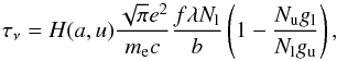 (A.1)where
H(a,u) is the Voigt function, a and
u being functions of the frequency ν and the Doppler
width b. e and me are the
charge and mass of the electron, respectively, f is the oscillator
strength, λ the central rest-frame wavelength of the transition,
N the column density, g the statistical weight of the
level, and subscripts l and u indicate the lower and upper level, respectively, of the
transition in question. The flux arriving at a particular layer is determined at the line
centre of the transition. As long as the absorption line is still in the optically thin
regime, this is equal to integrating the flux over the line profile. However, the
line-centre flux starts to diverge from the profile-averaged flux at larger optical
depths. The ratio of these fluxes depends on the optical depth only (and not, as one might
expect, on the b-parameter of the absorbing medium) and we can therefore
easily convert the flux at line centre to a profile-averaged flux at any optical depth
through tabulation of this ratio at a range of optical depths.
(A.1)where
H(a,u) is the Voigt function, a and
u being functions of the frequency ν and the Doppler
width b. e and me are the
charge and mass of the electron, respectively, f is the oscillator
strength, λ the central rest-frame wavelength of the transition,
N the column density, g the statistical weight of the
level, and subscripts l and u indicate the lower and upper level, respectively, of the
transition in question. The flux arriving at a particular layer is determined at the line
centre of the transition. As long as the absorption line is still in the optically thin
regime, this is equal to integrating the flux over the line profile. However, the
line-centre flux starts to diverge from the profile-averaged flux at larger optical
depths. The ratio of these fluxes depends on the optical depth only (and not, as one might
expect, on the b-parameter of the absorbing medium) and we can therefore
easily convert the flux at line centre to a profile-averaged flux at any optical depth
through tabulation of this ratio at a range of optical depths.
When considering a cloud with a non-zero size, the layers will be separated by a distance equal to the cloud size divided by the number of layers minus one, and the decrease of the flux with distance is taken into account from layer to layer. We also calculate the flux decrease due to H i absorption at Lyα, Lyβ, Lyγ, Lyδ and Lyϵ, for (excitation) transitions that are near these wavelengths. The resulting population of the ion levels due to photo-excitation is calculated as described in Vreeswijk et al. (2007) and Vreeswijk (2011, see also Sect. 3.1) for each relevant sublayer.
For ionization, the optical depth is τ = Nσ, and we
calculate the sub-layer ionization rate as:  (A.2)where
σν,subshell is the cross section (in
cm2) of a particular subshell of an ion. The cross sections of the inner
shells are taken from Verner et al. (1993) and
Verner & Yakovlev (1995)9, while the cross sections for the outer shells are
taken from Verner et al. (1996). The integration
interval, set by Eth and Emax, is
also defined in these references. The total ionization rate of each sublayer is obtained
by summing the rates of the different ion subshells. The decrease in the sublayer column
density due to ionization is determined using
dNsublayer = RsublayerNsublayer.
For ions with excited-level populations (e.g. Fe ii and Fe iii), we
assume that the ionization cross section is independent of the excitation level of the
ion, i.e. the fraction of ionizations from each level is considered to be the same.
(A.2)where
σν,subshell is the cross section (in
cm2) of a particular subshell of an ion. The cross sections of the inner
shells are taken from Verner et al. (1993) and
Verner & Yakovlev (1995)9, while the cross sections for the outer shells are
taken from Verner et al. (1996). The integration
interval, set by Eth and Emax, is
also defined in these references. The total ionization rate of each sublayer is obtained
by summing the rates of the different ion subshells. The decrease in the sublayer column
density due to ionization is determined using
dNsublayer = RsublayerNsublayer.
For ions with excited-level populations (e.g. Fe ii and Fe iii), we
assume that the ionization cross section is independent of the excitation level of the
ion, i.e. the fraction of ionizations from each level is considered to be the same.
When Fe ii is ionized by removal of an inner-shell electron, i.e. one that is not in the outer 3d or 4s shells, it is generally not converted to Fe iii. The vacancy created in the inner shell is filled by a cascade of radiative (fluorescent) and non-radiative (Auger) transitions, which can cause additional electrons to be expelled. The total number of electrons that are removed following ionization of an electron in a particular shell has been calculated for various ions and ionization states by Kaastra & Mewe (1993), whose results we apply in our programme. In practice, practically all Fe ii ions that are converted to Fe iii are due to outer shell (3d or 4s) ionizations. We also note that although higher energy photons (up to several tens of keV) can ionize Fe ii, the majority of ionizations are caused by lower energy photons (from the ionization threshold of 16.2 eV up to a few hundred electron-volts). However, the higher energy photons become more important with increasing H i column density, as the hydrogen atoms become more and more effective at shielding Fe ii and other ions from the lower energy ionizing photons. We stress that although we are mentioning Fe ii and Fe iii here, the same applies to any other ion that is included, such as Si ii, C ii and Cr ii.
Since our calculations involve ionization of Fe ii as well as the population of excited levels of Fe iii, we need to take into account that after ionization of Fe ii to Fe iii, the latter will not necessarily be in its ground state immediately. Since these are non-standard calculations and important for our modelling of the GRB 080310 column densities, they are described in Sect. 3.2.2.
After a packet of photons (ΔtFν) has travelled through all the layers in the cloud along the sightline, ionizing and exciting ions along its path, the remaining column densities (ground state and, if relevant, excited levels) in each layer are updated to be used for the next packet coming through. At each time step, the total ground-state and excited-level column densities are determined by simply adding up all layer column densities, which can be compared to measurements.
All Tables
Cross sections for ionization of ground-term Fe ii ions to different excited levels of Fe iii, as calculated with the FAC and Cowan codes.
Maximum Fe iii column
density reached as a function of the assumed H i column and iron abundance in
the GRB 080310 absorber.
All Figures
|
Fig. 1 Light curves in V (bottom), R, I (top) and the clear filter as recorded by the RAPTOR-T telescope. The magnitudes have not been corrected for the Galactic foreground extinction. The four epochs at which the UVES spectra were taken are indicated with the grey vertical bands. |
| In the text | |
|
Fig. 2 Photo-excitation modelling of the observed (total) column densities as a function
of time, as measured in Paper I (see their Table 3), for C ii,
Si ii, Fe ii and Fe iii. The open circles are
detections, while the open triangles indicate upper or lower limits
(3σ). The different colours denote the different ion levels:
black for the ground state and red-green-maroon-orange for the first four excited
levels, while the Fe ii |
| In the text | |
|
Fig. 3 Adopted input flux spectrum that is arriving at the GRB-facing side of the observed cloud (in observed flux units) depicted at two different epochs: tobs = 225 s on the left and tobs = 672 s on the right. The solid line shows the default input spectrum with a spectral slope of β = −0.75 up to 0.3 keV, above which the X-ray flux (at 1.73 keV) and spectral slope is adopted. The RAPTOR VRI and Swift XRT observations corresponding to these epochs are overplotted with open squares. The long-dashed line shows the default input spectrum modified by an extinction of AV = 0.19 mag; since this extinction is placed inside the observed cloud, it is not observable at the front of the cloud. The dotted line shows the input spectrum assuming a spectral slope of β = −1, combined with no extinction. The dashed line between the observed optical and X-ray regimes shows our approximation to the Littlejohns model flux. The energy and flux limits of this figure are the same as those in Fig. 9 of Littlejohns et al. (2012) for easy comparison. The hashed regions show the flux decrease due to a foreground cloud with H i column density log N(H i) = 18.9 for the default input flux model (horizontal lines) and log N(H i) = 20.3 for the alternative Littlejohns input spectrum (vertical lines); see Sect. 4 and Table 3 for more details. The ionization edges of He i at 24 eV/(1+z) and He ii at 54 eV/(1+z) can be spotted. We note that the spectral region between the Lyman limit and the X-ray data is not constrained by imaging observations. |
| In the text | |
|
Fig. 4 Partial energy level (or Grotrian) diagram for the relevant lower terms of the three lowest configurations of Fe iii: 3d6, 3d54s and 3d54p (indicated at the top). The horizontal solid lines depict the energy levels, labelled with the term and J-value. Selected transitions are shown with dotted lines between levels. For each transition, we list the logarithm of the transition probability (or Einstein A-coefficient, in (s-1)) of the strongest transition between the terms, adopting the Raassen & Uylings values (see Sect. 3.1). |
| In the text | |
|
Fig. 5 Photo-excitation and -ionization modelling of the observed (total) column densities as a function of time, as measured by De Cia et al. (2012) (see Table 3 of Paper I), for H i, C ii, Si ii, Cr ii, Fe ii and Fe iii (from top to bottom panels). The solid and dotted lines correspond to the best-fitting model, assuming the default and the Littlejohns input flux, respectively. The different colours of the symbols and lines have the same meaning as in Fig. 2. Although overall the model provides a reasonable description of the column density evolution, the observed excited levels of Fe ii at epoch II are significantly underestimated. See the text and Table 3 for more details. |
| In the text | |
|
Fig. 6 Same as Fig. 5, but including a foreground cloud situated between the GRB and the observed absorber. The solid and dotted lines correspond to the best-fitting model, assuming the default and Littlejohns input flux, respectively. The foreground absorber is mostly ionized by the time of the second epoch UVES spectrum and can therefore escape a clear detection. See the text and Table 3 for more details. |
| In the text | |
Current usage metrics show cumulative count of Article Views (full-text article views including HTML views, PDF and ePub downloads, according to the available data) and Abstracts Views on Vision4Press platform.
Data correspond to usage on the plateform after 2015. The current usage metrics is available 48-96 hours after online publication and is updated daily on week days.
Initial download of the metrics may take a while.