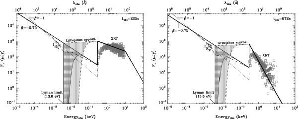
Adopted input flux spectrum that is arriving at the GRB-facing side of the observed cloud (in observed flux units) depicted at two different epochs: t_obs = 225 s on the left and t_obs = 672 s on the right. The solid line shows the default input spectrum with a spectral slope of β = −0.75 up to 0.3 keV, above which the X-ray flux (at 1.73 keV) and spectral slope is adopted. The RAPTOR VRI and Swift XRT observations corresponding to these epochs are overplotted with open squares. The long-dashed line shows the default input spectrum modified by an extinction of A_V = 0.19 mag; since this extinction is placed inside the observed cloud, it is not observable at the front of the cloud. The dotted line shows the input spectrum assuming a spectral slope of β = −1, combined with no extinction. The dashed line between the observed optical and X-ray regimes shows our approximation to the Littlejohns model flux. The energy and flux limits of this figure are the same as those in Fig. 9 of Littlejohns et al. (2012) for easy comparison. The hashed regions show the flux decrease due to a foreground cloud with H i column density log N(H i) = 18.9 for the default input flux model (horizontal lines) and log N(H i) = 20.3 for the alternative Littlejohns input spectrum (vertical lines); see Sect. 4 and Table 3 for more details. The ionization edges of He i at 24 eV/(1+z) and He ii at 54 eV/(1+z) can be spotted. We note that the spectral region between the Lyman limit and the X-ray data is not constrained by imaging observations.