| Issue |
A&A
Volume 548, December 2012
|
|
|---|---|---|
| Article Number | L3 | |
| Number of page(s) | 4 | |
| Section | Letters | |
| DOI | https://doi.org/10.1051/0004-6361/201220595 | |
| Published online | 22 November 2012 | |
XMM-Newton observations of SNR 1987A
II. The still increasing X-ray light curve and the properties of Fe K lines⋆
1
Max-Planck-Institut für extraterrestrische Physik,
Postfach 1312, Giessenbachstr.,
85741
Garching,
Germany
e-mail: pmaggi@mpe.mpg.de
2
MIT Kavli Institute, Cambridge, MA
02139,
USA
Received: 19 October 2012
Accepted: 6 November 2012
Aims. We report on the recent observations of the supernova remnant SNR 1987A in the Large Magellanic Cloud with XMM-Newton. Carefully monitoring the evolution of the X-ray light curve allows us to probe the complex circumstellar medium structure observed around the supernova progenitor star.
Methods. We analysed all XMM-Newton observations of SNR 1987A from January 2007 to December 2011, using data from the EPIC-pn camera. Spectra from all epochs were extracted and analysed in a homogeneous way. Using a multi-shock model to fit the spectra across the 0.2–10 keV bandm we measured soft and hard X-ray fluxes with high accuracy. In the hard X-ray band we examined the presence and properties of Fe K lines. Our findings have been interpreted in the framework of a hydrodynamics-based model.
Results. The soft X-ray flux of SNR 1987A has continuously increased in recent years. Although the light curve shows a mild flattening, there is no sudden break as reported in an earlier work, a picture echoed by a revision of the Chandra light curve. We therefore conclude that material in the equatorial ring and out-of-plane H ii regions are still being swept up. We estimate the thickness of the equatorial ring to be at least 4.5 × 1016 cm (0.0146 pc). This lower limit will increase as long as the soft X-ray flux has not reached a turn-over. We detect a broad Fe K line in all spectra from 2007 to 2011. The widths and centroid energies of the lines indicate there is a collection of iron ionisation stages. Thermal emission from the hydrodynamic model does not reproduce the low-energy part of the line (6.4–6.5 keV), suggesting that fluorescence from neutral and/or low ionisation Fe might be present.
Key words: ISM: individual objects: SN 1987A / X-rays: ISM / ISM: supernova remnants / Magellanic Clouds
© ESO, 2012
1. Introduction
SNR 1987A is one of the most studied objects in the southern sky. Because of its location in the Large Magellanic Cloud (LMC) at a distance of 50 kpc, it can be resolved at radio, optical, and even X-ray wavelengths. X-ray observatories such as ROSAT, Chandra, and XMM-Newton have frequently observed SNR 1987A, offering a unique opportunity to follow the early evolution of supernova remnant (SNR).
The most important feature of the soft X-ray light curve (between 0.5 and 2 keV) has been the upturn observed about 6000 days after the explosion (Park et al. 2005), interpreted as the beginning of the interaction of the blast wave with an “equatorial ring” (ER) of denser material around the progenitor star (see for instance Fig. 7 in Sugerman et al. 2002). The ER is likely to have been formed by the interaction between the stellar winds emitted by the progenitor star during its red supergiant and blue supergiant phases (e.g. Chevalier & Dwarkadas 1995), although binary merger models also exist to explain such a structure (e.g. Morris & Podsiadlowski 2007). Monitoring the evolution of the X-ray light curve allows probing the structure of the ring and constraining the late stages of the progenitor. Dewey et al. (2012, hereafter D12 present simple hydrodynamic models that reproduce the soft and hard X-ray light curves. The models show the soft X-ray flux behaviour for both the case where the forward shock has left the ER and the case where the ER is still being shocked (the “thin” and “thick” cases in their Fig. 12).
Park et al. (2011, hereafter P11 present recent Chandra observations (up to September 2010). Owing to the apparent flattening of the soft X-ray light curve, these authors conclude that SNR 1987A had reached a new evolutionary phase, where the blast wave has passed the main body of the ER and is now interacting with matter with a decreasing density gradient. However, Helder et al. (2012, hereafter H12 used the revised ACIS calibration to analyse all Chandra observations (including new ones, up to March 2012). They conclude that the sudden break reported by P11 was only a calibration effect.
In this Letter, we present our latest XMM-Newton monitoring observations (Sect. 2). We focus first on the evolution of the X-ray flux (Sect. 3), then report the detection of Fe K lines (Sect. 4). Discussion and conclusions are given in Sect. 5.
Details of the XMM-Newton EPIC-pn observations.
2. Observations and data reduction
The X-ray photons from SNR 1987A were amongst the first XMM-Newton detected in January 2000. This observation and two others from 2001 and 2003 were analysed by Haberl et al. (2006). We then started a yearly monitoring of SNR 1987A, from Januray 2007 (Heng et al. 2008) to December 2011. The high-resolution Reflection Grating Spectrometer (RGS) data taken up to January 2009 are presented in Sturm et al. (2010).
Here we homogeneously (re-)analyse all observations from 2007 to 2011, three of which have not been published so far. We mainly use data from the EPIC-pn camera (Strüder et al. 2001), operated in full-frame mode with medium filter. Details of the observations are listed in Table 1. We processed all observations with the SAS1 version 11.0.1. We extracted spectra from a circular region centred on the source, with a radius of 25′′. The background spectra were extracted from a nearby point-source-free region common to all observations. We selected single-pixel events (PATTERN = 0) from the pn detector. We rebinned the spectra with a minimum of 20 counts per bin in order to allow the use of the χ2-statistic. Non-rebinned spectra were used with the C-statistic (Cash 1979) for the study of Fe K lines (see Sect. 4), because of the limited photon statistics above 6 keV. The spectral fitting package XSPEC (Arnaud 1996) version 12.7.0u was used to perform the spectral analysis.
3. X-ray light curve
To measure the X-ray flux of SNR 1987A, we fitted the EPIC-pn spectra with a three-component plane-parallel shock model (called vpshock in XSPEC, where the prefix “v” indicates that abundances can vary), using neivers 2.0. This is the same model as the one used by D12 for Chandra and XMM-Newton spectra, with a fixed-temperature component (kT = 1.15 keV), although we did not use a Gaussian smoothing. This model gives slightly better fits than when using a two-component model (e.g. Park et al. 2004; Heng et al. 2008). The high- and low-temperature components are believed to originate from the interaction of the shocks with uniform material and denser clumps in the ER, respectively (D12). Another interpretation is that the high-temperature component comes from plasma shocked a second time by a reflected shock (Zhekov et al. 2006).
For elemental abundances, we followed the same procedure as in Haberl et al. (2006): N, O, Ne, Mg, Si, S, and Fe abundances were allowed to vary but were the same for all observations, whereas the He, C, Ar, Ca, and Ni abundances were fixed. The systemic velocity of SNR 1987A (286 km s-1, e.g. Gröningsson et al. 2008) was taken into account by choosing the redshift accordingly.
For the absorption of the source emission, we included two photoelectric absorption components, one with NH Gal = 0.6 × 1021 cm-2 (fixed) for the Galactic foreground absorption (Dickey & Lockman 1990) and another one with NH LMC (free in the fit) for the LMC. Metal abundances for the second absorption component are fixed to the average metallicity in the LMC (i.e., half the solar values, Russell & Dopita 1992). All spectra share the same NH LMC.
We simultaneously fitted the six spectra using energies between 0.2 and 10 keV. For consistency with the detection of Fe K lines (see Sect. 4), we included an additional (Gaussian) line to the model for the spectra obtained after 2007. The central energies and widths of the lines were fixed to the values found in the detailed analysis (Sect. 4). Only the normalisation of each line was left free.
The fit was satisfactory, with χ2 = 4125.06 for 3443 degrees of freedom. Although detailed spectral fits are not the focus of this study, we found that (i) the best-fit NH LMC was  cm-2, corresponding to a total absorption column of 3.7 × 1021 cm-2, somewhat higher than found using the grating instruments aboard Chandra and XMM-Newton (Sturm et al. 2010; Zhekov et al. 2006); (ii) the abundance pattern is in line with the one reported by Sturm et al. (2010) and D12; (iii) the temperature of the cool component increased only slightly from 0.34 to 0.38 keV, while its normalisation remained constant; and (iv) the temperature of the hot component is always in excess of 3.5 keV, and its normalisation and contribution steadily increased.
We measured the soft (0.5–2 keV) and hard (3–10 keV) fluxes at all epochs, using the XSPEC flux command. We list the results, with 3σ uncertainties (99.73% confidence level, C. L.) in Table 1. As is customary for SNR 1987A, we give absorbed fluxes, so comparisons between various observatories are easier (because they do not depend on the column densities obtained from the fit). The fluxes up to January 2009 are fully consistent with the results from Heng et al. (2008) and Sturm et al. (2010), which used the same data.
We included these results in the X-ray light curve shown in Fig. 1. Older XMM-Newton fluxes are taken from Haberl et al. (2006). We show the Chandra measurements with the old calibration (P11) and the newest one (H12). We also add the results from Suzaku observations (Sturm et al. 2009).
Within their respective errors, XMM-Newton, Chandra, and Suzaku measured soft and hard X-ray X-ray fluxes that agree very well. P11, using the ACIS calibration available at that time, stated that the soft X-ray flux from SNR 1987A has been nearly constant after day ~8000. Obviously XMM-Newton observed a source that was not constant, although we do observe a mild flattening of the light curve. The increase rates of the soft X-ray flux (last column of Table 1) vary from one year to another, showing that the evolution of the X-ray flux is not smooth. One should therefore be cautious when claiming a steepening or flattening of the light curve and wait for a longer baseline.
The discrepancy between Chandra and XMM-Newton measurements after day 8000 is reconciled by H12, using the revised Chandra calibration. They conclude that the apparent break in the soft X-ray light curve (P11) was mainly due to build-up of contamination on the ACIS optical blocking filters.
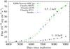 |
Fig. 1 Light curve of SNR 1987A in the soft and hard X-ray ranges. XMM-Newton data points (black diamonds) after day 7000 are given with 99.73% C. L. error bars. Updated Chandra measurements (with 68% C. L. errors, H12) and those based on the older calibration (with 90% C. L. errors, P11) are shown in green and grey, respectively. Suzaku measurements (Sturm et al. 2009, blue triangles) are also shown. |
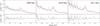 |
Fig. 2 Recent EPIC-pn spectra of SNR 1987A in the 5–8 keV range, showing the Fe K lines. The model used (red) is the sum of two components: a bremsstrahlung continuum and a Gaussian, shown by dotted lines. The bottom panels show the fit residuals. All panels have the same scale. For plotting purpose only, adjacent bins are rebinned in order to have a significant (≥ 5σ) detection in each rebinned channel. The feature seen at ~7.4 keV in the 2011 spectrum is an instrumental artefact and not an Ni K line. |
4. Fe K lines
The superior high-energy effective area of XMM-Newton (~900 cm-2 at 6.4 keV vs. ~200 cm-2 for Chandra) allows the study of Fe K lines with the EPIC cameras at energies between 6.4 and 6.7 keV, i.e. out of the range covered by RGS. Heng et al. (2008) note a possible detection of an Fe Kα line in the spectrum obtained in 2007, but the insufficient statistics precluded a more detailed analysis. In the coadded spectra from 2007 to January 2009, Sturm et al. (2010) identified a line at 6.57 ± 0.08 keV.
We analysed the presence and properties of Fe K lines in all the monitoring observations (Table 1). We fitted the non-rebinned spectra with a bremsstrahlung continuum and a Gaussian line, making use of the C-statistic to take the limited number of counts in each bin into account. We performed F-tests to evaluate the significance of the line in each observation: we found a detection more than 3σ significant in the data from 2008 and 2011, and more than 4σ significant in the spectra from December 2009 and 2010. The January 2009 observation, having a slightly shorter exposure due to longer high background activity periods, still yields a 2σ detection. We found only a marginal (1σ) detection in the 2007 spectrum, in agreement with previous studies.
We show the lines in the three unpublished spectra in Fig. 2. The plasma temperatures of the bremsstrahlung continua range from kT = 2.75 to 3 keV, and the emission measures follow the increasing trend of the hard X-ray flux. Line properties are given in Table 2 for all observations except the one from 2007.
Fe K line properties.
No evolution of the line central energy is found within the uncertainties, but our spectra suffer from limited statistics. The energy of the Fe K line depends on the ionisation stage of iron, increasing from 6.4 keV for Fe ii, to 6.7 keV for Fe xxv (Makishima 1986; Kallman et al. 2004). The spectral resolution is only ~160 eV (Strüder et al. 2001), so we are not able to resolve possible contributions from different Fe ions present in the X-ray emitting plasma. Therefore, the large measured widths of the lines in our spectra are most likely a sum of lines (which might be Doppler-broadened) from several Fe ions, convolved with the instrumental response of the camera. The weighted average of the emission-line centroids (6.60 ± 0.01 keV) and the typical widths (~100 eV) indicate the presence of ionisation stages from Fe xvii to Fe xxiv. This is consistent with the detection of lines from Fe xvii to Fe xx in the RGS spectra (Sturm et al. 2010), and the detection of an Fe xxii–Fe xxiii blend in the Chandra High Energy Transmission Grating spectra (Dewey et al. 2008).
The flux in the iron line indicates an increase around day 8000, and a decrease afterwards. However, given the large (statistical) errors in the flux measurements, we cannot exclude the possibility that the flux of the line remained constant in the past three years. Since the hard continuum steadily increased during that period of time, the equivalent width of the line decreased in the last observations (Table 2).
5. Discussion and conclusions
Our monitoring campaign with XMM-Newton since 2007 is ideally suited to following the evolution of SNR 1987A: (i) we used the same intrument settings (observing mode, filter, read-out time), (ii) we extracted the spectra in the same regions, and (iii) we used the same model for all the spectra. The high throughput of XMM-Newton results in the high statistical quality of our spectra. This allows high-confidence flux measurements with relatively small errors and free of cross-calibration problems due to different observing modes.
Our light curve shows a continuous increase in the soft X-ray flux of SNR 1987A, indicating that no turn-over has been reached yet and that the blast wave is still propagating into dense regions of the ER. To further constrain the thickness of the ER, given the continuous increase in the soft X-ray flux, we use the “2 × 1D” hydrodynamical model from D12. The recent XMM-Newton and Chandra measurements point towards a thickness of at least 4.5 × 1016 cm (0.0146 pc) for the ER, and each year of continued flux increase requires an additional ER thickness of ~0.53 × 1016 cm (0.0017 pc).
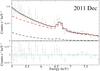 |
Fig. 3 Details of the Fe K lines region of the spectrum from December 2011. The model used is the three-shock components model described in Sect. 3, including emission from Fe below He-like ions and without a Gaussian line. The “hot” component (red dashed line) dominates the continuum and line spectrum but does not account for an emission excess around 6.55 keV. |
The high-energy collective power of XMM-Newton allowed us to detect and characterise the Fe K lines from SNR 1987A. We found that the energies and the widths of the lines imply the presence of a collection of ionisation stages for iron. To investigate which model component is most responsible for the Fe K lines, we used the best-fit three-shock model (switching off the Gaussian line) and using the NEI version 1.1, as it includes low ionisation stages (below He-like ions), which allows the whole range of energy between 6.4 and 6.7 keV to be probed as a function of kT and τ (see Fig. 3 in Furuzawa et al. 2009). As expected, we found that only the high-temperature component significantly contributes to the hard continuum and the line. When including emission from ions below He-like iron, the shapes and fluxes of the lines from the high-temperature component (Fig. 3) fail to reproduce the data. There is need for lower ionisation stages to explain the excess observed at ~6.55 keV. This points to the presence of shocked material with shorter ionisation ages τ. In the framework of the hydrodynamics-based model from D12, we find that the main contribution to the Fe K emission therefore comes from the out-of-plane material (“H ii region”), which has a temperature and ionisation age that produces emission in the 6.55–6.61 keV range. Another possibility for the low-energy emission (~6.4 keV) is fluorescence from near-neutral Fe, including Fe in the unshocked ejecta. Material in the dense
ER clumps, on the other hand, has a temperature that is too low to significantly contribute to the line.
Following the evolution of the Fe K line fluxes and centroid energies is crucial to constraining their origin. Next-generation instrumentation, such as the X-ray calorimeter aboard Astro-H, will be able to resolve lines from different Fe ions, thus providing even deeper physical insights.
The calibration issues encountered by the Chandra team show how important it is to use both observatories to monitor such an important source. To follow the evolution of the light curve and of the iron lines, subsequent observations of SNR 1987A with XMM-Newton are highly desirable.
Science Analysis Software, http://xmm.esac.esa.int/sas/
Acknowledgments
The XMM-Newton project is supported by the Bundesministerium für Wirtschaft und Technologie / Deutsches Zentrum für Luft- und Raumfahrt (BMWi/DLR, FKZ 50 OX 0001) and the Max-Planck Society. P. M. and R. S. acknowledge support from the BMWi/DLR grants FKZ 50 OR 1201 and FKZ 50 OR 0907, respectively.
References
- Arnaud, K. A. 1996, in Astronomical Data Analysis Software and Systems V, eds. G. H. Jacoby, & J. Barnes, ASP Conf. Ser., 101, 17 [Google Scholar]
- Cash, W. 1979, ApJ, 228, 939 [NASA ADS] [CrossRef] [Google Scholar]
- Chevalier, R. A., & Dwarkadas, V. V. 1995, ApJ, 452, L45 [NASA ADS] [CrossRef] [Google Scholar]
- Dewey, D., Zhekov, S. A., McCray, R., & Canizares, C. R. 2008, ApJ, 676, L131 [NASA ADS] [CrossRef] [Google Scholar]
- Dewey, D., Dwarkadas, V. V., Haberl, F., Sturm, R., & Canizares, C. R. 2012, ApJ, 752, 103 [NASA ADS] [CrossRef] [Google Scholar]
- Dickey, J. M., & Lockman, F. J. 1990, ARA&A, 28, 215 [NASA ADS] [CrossRef] [MathSciNet] [Google Scholar]
- Furuzawa, A., Ueno, D., Hayato, A., et al. 2009, ApJ, 693, L61 [NASA ADS] [CrossRef] [Google Scholar]
- Gröningsson, P., Fransson, C., Leibundgut, B., et al. 2008, A&A, 492, 481 [NASA ADS] [CrossRef] [EDP Sciences] [Google Scholar]
- Haberl, F., Geppert, U., Aschenbach, B., & Hasinger, G. 2006, A&A, 460, 811 [NASA ADS] [CrossRef] [EDP Sciences] [Google Scholar]
- Helder, E. A., Broos, P. S., Dewey, D., et al. 2012, ApJ, submitted [Google Scholar]
- Heng, K., Haberl, F., Aschenbach, B., & Hasinger, G. 2008, ApJ, 676, 361 [NASA ADS] [CrossRef] [Google Scholar]
- Kallman, T. R., Palmeri, P., Bautista, M. A., Mendoza, C., & Krolik, J. H. 2004, ApJS, 155, 675 [NASA ADS] [CrossRef] [Google Scholar]
- Makishima, K. 1986, in Lecture Notes in The Physics of Accretion onto Compact Objects, eds. K. O. Mason, M. G. Watson, & N. E. White Physics (Berlin: Springer Verlag), 266, 249 [Google Scholar]
- Morris, T., & Podsiadlowski, P. 2007, Science, 315, 1103 [NASA ADS] [CrossRef] [Google Scholar]
- Park, S., Zhekov, S. A., Burrows, D. N., Garmire, G. P., & McCray, R. 2004, ApJ, 610, 275 [NASA ADS] [CrossRef] [Google Scholar]
- Park, S., Zhekov, S. A., Burrows, D. N., & McCray, R. 2005, ApJ, 634, L73 [NASA ADS] [CrossRef] [Google Scholar]
- Park, S., Zhekov, S. A., Burrows, D. N., et al. 2011, ApJ, 733, L35 [NASA ADS] [CrossRef] [Google Scholar]
- Russell, S. C., & Dopita, M. A. 1992, ApJ, 384, 508 [NASA ADS] [CrossRef] [Google Scholar]
- Strüder, L., Briel, U., Dennerl, K., et al. 2001, A&A, 365, L18 [NASA ADS] [CrossRef] [EDP Sciences] [Google Scholar]
- Sturm, R., Haberl, F., Hasinger, G., Kenzaki, K., & Itoh, M. 2009, PASJ, 61, 895 [NASA ADS] [Google Scholar]
- Sturm, R., Haberl, F., Aschenbach, B., & Hasinger, G. 2010, A&A, 515, A5 [NASA ADS] [CrossRef] [EDP Sciences] [Google Scholar]
- Sugerman, B. E. K., Lawrence, S. S., Crotts, A. P. S., Bouchet, P., & Heathcote, S. R. 2002, ApJ, 572, 209 [NASA ADS] [CrossRef] [Google Scholar]
- Zhekov, S. A., McCray, R., Borkowski, K. J., Burrows, D. N., & Park, S. 2006, ApJ, 645, 293 [NASA ADS] [CrossRef] [Google Scholar]
All Tables
All Figures
|
Fig. 1 Light curve of SNR 1987A in the soft and hard X-ray ranges. XMM-Newton data points (black diamonds) after day 7000 are given with 99.73% C. L. error bars. Updated Chandra measurements (with 68% C. L. errors, H12) and those based on the older calibration (with 90% C. L. errors, P11) are shown in green and grey, respectively. Suzaku measurements (Sturm et al. 2009, blue triangles) are also shown. |
| In the text | |
|
Fig. 2 Recent EPIC-pn spectra of SNR 1987A in the 5–8 keV range, showing the Fe K lines. The model used (red) is the sum of two components: a bremsstrahlung continuum and a Gaussian, shown by dotted lines. The bottom panels show the fit residuals. All panels have the same scale. For plotting purpose only, adjacent bins are rebinned in order to have a significant (≥ 5σ) detection in each rebinned channel. The feature seen at ~7.4 keV in the 2011 spectrum is an instrumental artefact and not an Ni K line. |
| In the text | |
|
Fig. 3 Details of the Fe K lines region of the spectrum from December 2011. The model used is the three-shock components model described in Sect. 3, including emission from Fe below He-like ions and without a Gaussian line. The “hot” component (red dashed line) dominates the continuum and line spectrum but does not account for an emission excess around 6.55 keV. |
| In the text | |
Current usage metrics show cumulative count of Article Views (full-text article views including HTML views, PDF and ePub downloads, according to the available data) and Abstracts Views on Vision4Press platform.
Data correspond to usage on the plateform after 2015. The current usage metrics is available 48-96 hours after online publication and is updated daily on week days.
Initial download of the metrics may take a while.