| Issue |
A&A
Volume 548, December 2012
|
|
|---|---|---|
| Article Number | A31 | |
| Number of page(s) | 6 | |
| Section | Cosmology (including clusters of galaxies) | |
| DOI | https://doi.org/10.1051/0004-6361/201220278 | |
| Published online | 15 November 2012 | |
Cosmology with Hu-Sawicki gravity in the Palatini formalism
1
Observatório Nacional,
20921-400
Rio de Janeiro –,
RJ,
Brazil
e-mail: thoven@on.br; campista@on.br; alcaniz@on.br
2
Departamento de Física, Universidade Federal do Rio Grande do
Norte, 59072-970
Natal –
RN,
Brazil
e-mail: janilo@dfte.ufrn.br
Received:
23
August
2012
Accepted:
12
September
2012
Cosmological models based on f(R)-gravity may exhibit a natural acceleration mechanism without introducing a dark energy component. We investigate cosmological consequences of the so-called Hu-Sawicki f(R) gravity in the Palatini formalism. We derived theoretical constraints on the model parameters and performed a statistical analysis to determine the parametric space allowed by current observational data. We find that this class of models is indistinguishable from the standard ΛCDM model at the background level. In contrast to previous results achieved with the metric approach, we show that these scenarios are able to produce the sequence of radiation-dominated, matter-dominated, and accelerating periods without need of dark energy.
Key words: gravitation / cosmological parameters / cosmology: observations / cosmology: theory / dark energy
© ESO, 2012
1. Introduction
General relativity (GR) is a very well-tested and established theory of gravity. However, all successful tests performed so far do not account for the ultra-large scales corresponding to the low-curvature characteristics of the Hubble radius today. Therefore, it is in principle conceivable that the recent discovery of the late-time cosmic acceleration (Eisenstein et al. 2005; Perlmutter et al. 1999; Riess et al. 1998, 1999; Spergel et al. 2003) could be explained by modifying Einstein’s GR in the far-infrared regime. Although the diversity of approaches is the hallmark in this field (see, e.g., Alves et al. 2010; Banados & Ferreira 2010; Basilakos et al. 2011; Bengochea & Ferraro 2009; Clifton et al. 2012; Mukohyama 2010; Pereira & Aguilar 2011; Trodden 2011), the simplest possible theory is achieved by adding terms proportional to powers of the Ricci scalar R to the Einstein-Hilbert Lagrangian, the so-called f(R) gravity (see Capozziello & De Laurentis 2011; De Felice & Tsujikawa 2010; Nojiri & Odintsov 2011; Sotiriou & Faraoni 2010, for recent reviews).
In contrast to the standard general relativistic scenario, f(R) cosmology can naturally drive an accelerating cosmic expansion without introducing dark energy. However, the freedom in the choice of different functional forms of f(R) gives rise to the problem of how to constrain the many possible f(R) gravity theories. In this regard, much effort has been expended so far, mainly from the theoretical viewpoint (Aktas et al. 2012; Alves et al. 2009; Cognola et al. 2009; Faraoni 2010; Harko 2010; Harko & Lobo 2010; Harko et al. 2011; Multamaki et al. 2010; Pereira et al. 2010; Santos 2010; Shamir 2010; Sharif & Kausar 2011a,b). General principles such as the so-called energy conditions (Atazadeh et al. 2009; Banijamali et al. 2012; Bertolami & Sequeira 2009; Garcia et al. 2011; Kung 1996; Santos et al. 2007, 2010a; Wu & Yu 2010), nonlocal causal structure (Clifton & Barrow 2005; Rebouças & Santos 2009, 2010; Santos et al. 2010b), and problems such as loop quantum cosmology (Cognola et al. 2005; Olmo & Sanchis-Alepuz 2011; Zhang & Ma 2011) have also been taken into account to clarify its subtleties. More recently, observational constraints from several cosmological data sets for testing the viability of these theories have also been explored (Borowiec et al. 2006; Koivisto 2006; Li & Chu 2006; Li et al. 2007, 2009; Masui et al. 2010; Movahed et al. 2007; Yang & Chen 2009; Zhang et al. 2012).
An important aspect that is worth emphasizing concerns the two different variational approaches that may be followed when one works with f(R) gravity, namely, the metric and the Palatini formalisms. In the metric formalism the connections are defined a priori as the Christoffel symbols of the metric and the variation of the action is taken with respect to the metric, whereas in the Palatini variational approach the metric and the affine connections are treated as independent fields and the variation is taken with respect to both (for a review on f(R) theories in the Palatini approach see Olmo 2011). The result is that in the Palatini approach the connections depend on the metric and also on the particular f(R), while in the metric formalism the connections depend only on the metric. We have then that the same f(R) leads to different spacetime structures.
These differences also extend to the observational aspects. For instance, we note that some cosmological models based on a power-law functional form in the metric formulation fail in reproducing the standard matter-dominated era followed by an acceleration phase (Amendola et al. 2007; see, however, Capozziello et al. 2006), whereas in the Palatini approach, some analyses have shown that these theories admit the three post inflationary phases of the standard cosmological model (Amarzguioui et al. 2006; Fay et al. 2007). Nevertheless, we do not yet clearly comprehend the properties of the Palatini formulation of f(R) gravity in other scenarios, and questions such as the Newtonian limit (Dominguez & Barraco 2004; Meng & Wang 2004; Sotiriou 2006) and the Cauchy problem (Capozziello & Vignolo 2009a; Faraoni 2009; Lanahan-Tremblay & Faraoni 2007) are still contentious (see, however, Capozziello & Vignolo 2009b,c). Another problem of the Palatini f(R) formulation concerns surface singularities of static spherically symmetric objects with polytropic equation of state (Barausse et al. 2008a,b,c; Olmo 2011). This problem has been reexamined in Kainulainen et al. (2007); Olmo (2008), where the authors showed that the singularities may have more to do with peculiarities of the polytropic equation of state used (e.g. its natural regime of validity) and the f(R) model chosen.
Although it is mathematically simpler than the metric formulation, the Palatini approach has received little attention from the point of view of cosmological tests. Following early works in this direction (Amarzguioui et al. 2006; Campista et al. 2011; Carvalho et al. 2008; Fay et al. 2007; Santos et al. 2008), we explore in this paper the cosmological consequences of a class of modified f(R) gravity, recently proposed by Hu & Sawicki (2007), in the Palatini formulation. Among a number of f(R) models discussed in the literature, this is designed to posses a chameleon mechanism that allows one to evade solar system constraints. The cosmological scenario that arises from the metric formalism of this model has been shown to satisfy the conditions needed to produce a cosmologically viable expansion history. To test the observational viability of this class of models in the Palatini approach, we used different types of observational data, namely: type Ia supernovae (SNe Ia) observations from the Union2.1 sample (Suzuki et al. 2012); estimates of the expansion rate at z ≠ 0, as discussed in Stern et al. (2010); current measurements of the product of the cosmic microwave background (CMB) acoustic scale ℓA with the position of the baryon acoustic oscillations (BAO) peak (Blake et al. 2011b), dubbed the CMB/BAO ratio; and measurements of the gas mass fraction in galaxy clusters (Ettori et al. 2009). We show that for a subsample of model parameters, the so-called Hu-Sawicki scenarios in the Palatini approach are indistinguishable from the standard ΛCDM model and are able to produce the sequence of radiation-dominated, matter-dominated, and accelerating periods without need of dark energy.
The organization of the paper is the following: in Sect. 2 we summarize both the Palatini formalism and the Hu-Sawicki gravity. We describe in Sect. 3 the H(z) and SNe Ia observational data used to perform our statistical analysis. In Sect. 4, we show the results from our analysis, including data from the gas mass fraction of galaxy clusters and the CMB/BAO ratio. Finally, Sect. 5 contains a summary of our conclusions.
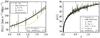 |
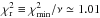
Fig. 1 (left) Predicted Hubble evolution H(z) as a function of the redshift for the Hu-Sawicki model in the Palatini formalism (Eqs. (5)–(8)). The curves correspond to the best-fit values of Ωm0 and c2 discussed in the text. For the sake of comparison, the standard ΛCDM model prediction is also shown. The data points are the measurements of the H(z) given in Stern et al. (2010). (right) Hubble diagram for 580 SNe Ia from the Union2.1 sample (Suzuki et al. 2012). The curves correspond to the best-fit values of Ωm0 and c2 displayed in Table 1. |
2. The Palatini approach
The modified Einstein-Hilbert action that defines an f(R)
gravity is given by 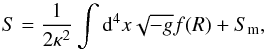 (1)where
κ2 = 8πG, g is the
determinant of the metric tensor and Sm is the standard action
for the matter fields.
(1)where
κ2 = 8πG, g is the
determinant of the metric tensor and Sm is the standard action
for the matter fields.
In the Palatini variational approach the fundamental idea is to regard the torsion-free
connection  , as well as the
metric gμν entering the action above, as two
independent fields. The field equations in this approach are
, as well as the
metric gμν entering the action above, as two
independent fields. The field equations in this approach are  (2)and
 (3)where
fR = df/dR
and
(3)where
fR = df/dR
and  represent covariant derivatives. From the above equations, we obtain the connections
 (4)where
 are the Christoffel
symbols of the metric. As mentioned above, the connections, and therefore the gravitational
fields, are described not only by the metric
gμν but also by the proposed
f(R) theory. As a cosmological model we consider a
homogeneous isotropic Universe described by the Friedmann-Lemaître-Robertson-Walker (FLRW)
flat geometry
gμν = diag(− 1,a2,a2,a2),
where a(t) is the cosmological scale factor, and as the
source of curvature a perfect-fluid with energy density ρ and pressure
p, whose energy-momentum tensor is given by
are the Christoffel
symbols of the metric. As mentioned above, the connections, and therefore the gravitational
fields, are described not only by the metric
gμν but also by the proposed
f(R) theory. As a cosmological model we consider a
homogeneous isotropic Universe described by the Friedmann-Lemaître-Robertson-Walker (FLRW)
flat geometry
gμν = diag(− 1,a2,a2,a2),
where a(t) is the cosmological scale factor, and as the
source of curvature a perfect-fluid with energy density ρ and pressure
p, whose energy-momentum tensor is given by
 .
.
The generalized Friedmann equation, obtained from Eqs. (2)–(4), can be written in
terms of the redshift z as 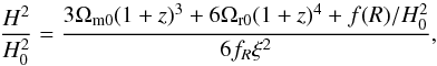 (5)where
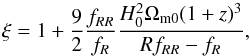 (6)and Ωm0 and
Ωr0 stand for the present-day values of the matter- and radiation-density
parameters. The trace of Eq. (2) results in
(6)and Ωm0 and
Ωr0 stand for the present-day values of the matter- and radiation-density
parameters. The trace of Eq. (2) results in
 (7)which we will consider in
order to restrict the parameters of the given f(R) theory.
(7)which we will consider in
order to restrict the parameters of the given f(R) theory.
2.1. The Hu-Sawicki gravity model
In this paper we are interested in the f(R) modified
gravity model proposed by Hu & Sawicki
(2007) (8)For
n = 1, the above equation can be rewritten as (Schmidt et al. 2009)
(8)For
n = 1, the above equation can be rewritten as (Schmidt et al. 2009)
 (9)where
Λ = m2c1/2c2
and
μ2 = m2/c2
are dimensionless parameters and
(9)where
Λ = m2c1/2c2
and
μ2 = m2/c2
are dimensionless parameters and  .
In the regime R ≫ μ2, this model is
practically indistinguishable from the ΛCDM scenario1. We have verified that the parameter n is completely
unconstrained by current data. Thus, without loss of generality and following Schmidt et al. (2009), we focus our analyses on the
case n = 1.
.
In the regime R ≫ μ2, this model is
practically indistinguishable from the ΛCDM scenario1. We have verified that the parameter n is completely
unconstrained by current data. Thus, without loss of generality and following Schmidt et al. (2009), we focus our analyses on the
case n = 1.
This model is intended to explain the current acceleration of the universe without
considering a cosmological constant term. Cosmological and astrophysical constraints on
the Hu-Sawicki gravity scenario in the metric formalism have been examined in a number of
papers (see, e.g., Ferraro et al. 2011; Gil-Marin et al. 2011; Li & Hu 2011; Lombriser et al.
2012; Martinelli 2009; Martinelli et al. 2009; Oyaizu et al. 2008). However, there is a complete lack of studies on the
mechanism of this proposal in the Palatini approach. Irrespective of the formalism
adopted, the model (8) must satisfy certain
viability conditions, for example, the positivity of the effective gravitational coupling,
which requires
κ2/fR > 0
(to avoid anti-gravity). For the current epoch, this condition implies
![\begin{equation} f_{R0} = \frac{ 3 + 2 \left( \frac{R_0}{m^2} \right)^2 c_2 }{ \frac{R_0}{m^2} \left[ 1 + 2 \left( \frac{R_0}{m^2} \right)c_2 \right] } > 0 , \end{equation}](/articles/aa/full_html/2012/12/aa20278-12/aa20278-12-eq40.png) (10)which corresponds to
the following bounds for the parameter c2:
(10)which corresponds to
the following bounds for the parameter c2:  (11)
(11)
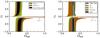 |
Fig. 2 (left) Contours of Δχ2 = 2.3 and Δχ2 = 6.17 in the Ωm0 × c2 plane arising from SNe Ia Union2.1 sample (Suzuki et al. 2012) (orange) and current H(z) data (Stern et al. 2010) (green). Black contours stand for the joint analysis involving these two sets of data. (right) Contours of Δχ2 = 6.17 in the Ωm0 × c2 plane when 7 measurements of the CMB/BAO ratio and 57 measurements of the gas mass fraction of galaxy clusters are added. We have also indicated the region fR0 < 0 corresponding to the bounds (11) for the best-fit values shown in Table 1. |
3. Observational constraints
To perform the observational tests discussed below, we solved Eq. (5) by taking the following steps: i) we first set z = 0 and computed c1 (in terms of c2 and R0) from Eq. (7); ii) we combined this result with Eq. (5) to obtain a solution for R0; iii) the value of R0 was then used as initial condition to solve Eq. (7) by using a fourth-order Runge-Kutta method and, finally, to obtain the function H(z), as given by Eq. (5).
Figure 1 shows the evolution of the Hubble parameter
and the predicted distance modulus
μ(z) = 5log [dL(z)/Mpc] + 25,
where  stands for the luminosity distance, as a function of redshift for some best-fit values for
Ωm0 and c2 obtained in our analyses (see Table
1). For the sake of comparison, the standard ΛCDM
prediction with Ωm0 = 0.26 is also shown (dashed line).
stands for the luminosity distance, as a function of redshift for some best-fit values for
Ωm0 and c2 obtained in our analyses (see Table
1). For the sake of comparison, the standard ΛCDM
prediction with Ωm0 = 0.26 is also shown (dashed line).
3.1. Expansion rate
To test the observational viability of the f(R)
scenario described by Eq. (8), we firstly
used current measurements of the expansion rate at z ≠ 0. Currently, this
test is based on the fact that luminous red galaxies (LRGs) can provide us with direct
measurements of H(z) (Jimenez & Loeb 2002; see also Zhang
& Ma 2010, for a recent review on H(z)
measurements from different techniques). This can be done by calculating the derivative of
cosmic time with respect to redshift, i.e.,  .
This method was first presented in Jimenez & Loeb
(2002) and consists of measuring the age difference between two red galaxies at
different redshifts to obtain the rate
Δz/Δt. By using a recently released
sample from the Gemini Deep Survey (GDDS) (McCarthy et al.
2004) and archival data (Dunlop et al.
1996; Nolan et al. 2001; Spinrad et al. 1997), Stern et al. (2010) have calculated 11 H(z)
data points over the redshift range 0.1 ≤ z ≤ 1.75.
.
This method was first presented in Jimenez & Loeb
(2002) and consists of measuring the age difference between two red galaxies at
different redshifts to obtain the rate
Δz/Δt. By using a recently released
sample from the Gemini Deep Survey (GDDS) (McCarthy et al.
2004) and archival data (Dunlop et al.
1996; Nolan et al. 2001; Spinrad et al. 1997), Stern et al. (2010) have calculated 11 H(z)
data points over the redshift range 0.1 ≤ z ≤ 1.75.
We estimated the free parameters P by using a χ2
statistics, i.e., ![\begin{equation} \label{eq:chi2.h} \chi_{\rm H}^2 = \sum_{i=1}^{N_{\rm H}} \frac{ \left[ H_i^\mathrm{th} (z_i|\mathbf{P}) - H_i^\mathrm{obs} (z_i) \right]^2 }{ \sigma^2_i } , \end{equation}](/articles/aa/full_html/2012/12/aa20278-12/aa20278-12-eq57.png) (12)where
(12)where
 is the theoretical Hubble
parameter at redshift zi and
σi is the uncertainty for each of the
NH = 11 determinations of
H(z) given in Stern et
al. (2010). In our analyses, the Hubble constant H0
was considered as a nuisance parameter and we marginalized over it.
is the theoretical Hubble
parameter at redshift zi and
σi is the uncertainty for each of the
NH = 11 determinations of
H(z) given in Stern et
al. (2010). In our analyses, the Hubble constant H0
was considered as a nuisance parameter and we marginalized over it.
Best-fit values for c2, c1 and fR0.
3.2. SNe Ia
The predicted distance modulus for a supernova at redshift z, given a
set of parameters P, is  , where
DL = H0dL
is the Hubble-free luminosity distance,
μ0 = 42.38−5log 10h and
h stands for the Hubble constant H0 in
units of 100 km s-1 Mpc-1. In our analysis, we used the latest
Union2.1 sample which includes 580 SNe Ia over the redshift range
0.015 ≤ z ≤ 1.414. To include the effect of systematic errors into our
analyses, we followed Suzuki et al. (2012) and
estimated the best fit and error bars to the set of parameters P by using a
χ2 statistics, with
, where
DL = H0dL
is the Hubble-free luminosity distance,
μ0 = 42.38−5log 10h and
h stands for the Hubble constant H0 in
units of 100 km s-1 Mpc-1. In our analysis, we used the latest
Union2.1 sample which includes 580 SNe Ia over the redshift range
0.015 ≤ z ≤ 1.414. To include the effect of systematic errors into our
analyses, we followed Suzuki et al. (2012) and
estimated the best fit and error bars to the set of parameters P by using a
χ2 statistics, with  (13)where C is a
580 × 580 covariance matrix (Suzuki et al. 2012).
In the same way as we did for the analysis involving
H(z) data, we also marginalized over
H0.
(13)where C is a
580 × 580 covariance matrix (Suzuki et al. 2012).
In the same way as we did for the analysis involving
H(z) data, we also marginalized over
H0.
4. Results
In Fig. 2 (left) we show the first results of our
statistical analyses. Contours corresponding to Δχ2 = 2.3 and
Δχ2 = 6.17 in the
Ωm0 × c2 plane are shown for the
χ2 given above. From this analysis, we clearly see that
neither the current H(z) and SNe Ia measurements alone nor
a combination of them ( )
can place tight constraints on the values of the f(R)
parameter c2. We also observed that other cosmological
observables seem to be unable to provide orthogonal contours to those shown in Fig. 2 (left), which in principle would lead to tighter bounds
on c2 from a joint analysis. Figure 2 (right) shows the results obtained when two other sets of cosmological
observations are included, namely: seven estimates of the ratio of the CMB acoustic scale
ℓA and the BAO peak, as given in Blake et al. (2011b), and the 57 measurements of the gas mass fraction in
X-ray luminous galaxy clusters discussed in Ettori et al.
(2009) (we refer the reader to Allen et al. (2002);
Blake et al. (2011a); Lima et al. (2003) for more details on these cosmologial tests). For this
joint analysis, the best-fit values are Ωm0 = 0.30 and
c2 = −0.25, with the reduced
)
can place tight constraints on the values of the f(R)
parameter c2. We also observed that other cosmological
observables seem to be unable to provide orthogonal contours to those shown in Fig. 2 (left), which in principle would lead to tighter bounds
on c2 from a joint analysis. Figure 2 (right) shows the results obtained when two other sets of cosmological
observations are included, namely: seven estimates of the ratio of the CMB acoustic scale
ℓA and the BAO peak, as given in Blake et al. (2011b), and the 57 measurements of the gas mass fraction in
X-ray luminous galaxy clusters discussed in Ettori et al.
(2009) (we refer the reader to Allen et al. (2002);
Blake et al. (2011a); Lima et al. (2003) for more details on these cosmologial tests). For this
joint analysis, the best-fit values are Ωm0 = 0.30 and
c2 = −0.25, with the reduced
 (ν
is defined as degrees of freedom), which is very close to the value found for the standard
ΛCDM model,
(ν
is defined as degrees of freedom), which is very close to the value found for the standard
ΛCDM model,  . This result clearly
shows that these scenarios are indistinguishable from each other at the background level,
which coincides with the analysis performed in the metric formalism and are discussed in
Martinelli et al. (2012) (although the expansion
histories for both metric and Palatini formalisms are completely different). It is worth
mentioning that in our analysis we considered both positive and negative values of the
f(R) parameter c2, in
agreement with the constraint (11). Note
also that for c2 = 0, the cosmological scenario discussed above
reduces to the Einstein-de Sitter model, which is ruled out by current data. We use the
joint best-fit value discussed above, as well as the others shown in Table 1, to discuss some cosmological consequences of this
class of f(R) cosmologies in the next section.
. This result clearly
shows that these scenarios are indistinguishable from each other at the background level,
which coincides with the analysis performed in the metric formalism and are discussed in
Martinelli et al. (2012) (although the expansion
histories for both metric and Palatini formalisms are completely different). It is worth
mentioning that in our analysis we considered both positive and negative values of the
f(R) parameter c2, in
agreement with the constraint (11). Note
also that for c2 = 0, the cosmological scenario discussed above
reduces to the Einstein-de Sitter model, which is ruled out by current data. We use the
joint best-fit value discussed above, as well as the others shown in Table 1, to discuss some cosmological consequences of this
class of f(R) cosmologies in the next section.
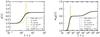 |
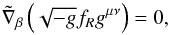
Fig. 3 Deceleration parameter (left) and effective equation of state (right) as a function of z for the best-fit values of Ωm0 and c2 presented in Table 1. The ΛCDM model is also shown for the sake of comparison. |
4.1. Cosmological consequences
Two important quantities directly related to the expansion rate of the Universe and its
derivatives are the deceleration parameter
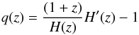 (14)and the effective
equation of state (EoS)
(14)and the effective
equation of state (EoS) 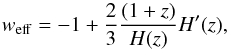 (15)where a prime denotes
differentiation with respect to z and
H(z) is given by Eq. (5). For all sets of best-fit values displayed in Table 1, we show q(z) and
weff(z) as a function of the redshift in
Fig. 3. Similarly to the analyses presented in Sect.
3, we have included a component of radiation
(Ωr0 = 5 × 10⁻⁵) to plot these curves. As can be seen from Fig.
3 (left), for some combinations of parameters the
cosmic evolution is well-behaved, with a past cosmic deceleration and a current
accelerating phase starting at z ≃ 1, which seems to agree well with
current kinematic analyses (see, e.g., Pires et al.
2010).
(15)where a prime denotes
differentiation with respect to z and
H(z) is given by Eq. (5). For all sets of best-fit values displayed in Table 1, we show q(z) and
weff(z) as a function of the redshift in
Fig. 3. Similarly to the analyses presented in Sect.
3, we have included a component of radiation
(Ωr0 = 5 × 10⁻⁵) to plot these curves. As can be seen from Fig.
3 (left), for some combinations of parameters the
cosmic evolution is well-behaved, with a past cosmic deceleration and a current
accelerating phase starting at z ≃ 1, which seems to agree well with
current kinematic analyses (see, e.g., Pires et al.
2010).
For all best-fit combinations shown in Table 1, Fig. 3 (right) shows that the Universe went through the last three phases of cosmological evolution, i.e., a radiation-dominated (weff = 1/3), a matter-dominated (weff = 0), and a late-time accelerating phase (weff < 0), which is similar to what happens in the standard ΛCDM cosmology. From these results, it is also clear that the arguments of Amendola et al. (2007) about the behavior of weff in the metric approach (we refer the reader to Capozziello et al. (2006) for a different conclusion) seems not to apply to the Palatini formalism, at least for the class of models discussed in this paper and the interval of parameters Ωm0 and c2 given by our statistical analysis – the same also happens to power-law (Amarzguioui et al. 2006; Carvalho et al. 2008; Fay et al. 2007; Santos et al. 2008) and exponential (Campista et al. 2011) f(R) gravities in the Palatini formalism. Moreover, in contrast to exponential-type f(R) models (see, e.g., Campista et al. 2011), we have not found solutions of transient cosmic acceleration in which the large-scale modification of gravity will drive the Universe to a new matter-dominated era in the future.
5. Conclusions
f(R)-gravity provides an alternative way to explain the current cosmic acceleration with no need of invoking either the existence of an extra spatial dimension or an exotic component of dark energy. Among a number of f(R) models discussed in the literature, the so-called Hu-Sawicki scenarios are designed to posses a chameleon mechanism that allows one to evade solar system constraints. Although the cosmological scenario that arises from the metric formalism of this model has been shown to satisfy the conditions needed to produce a cosmologically viable expansion history, its Palatini version had not yet been investigated and some interesting results in this way may still arise in the near future. It would be interesting, for example, to perform a cosmographic analysis in the Palatini formalism for this model, such as the one performed in the metric formalism by Capozziello et al. (2008). The combination of this task with the results shown here can improve the constraints of the Hu-Sawicki scenario and test its observational viability.
In this paper, we discussed several cosmological consequences of this class of models in
the Palatini formalism. We performed consistency checks and tested the observational
viability of these scenarios by using one of the latest SNe Ia data, the so-called Union2.1
sample, measurements of the expansion rate H(z) at
intermediary and high-z, estimates of the CMB/BAO ratio, and current
observations of the gas mass fraction in X-ray luminous galaxy clusters. We found a good
agreement between these observations and the theoretical predictions of the model, with the
reduced  for the
analyses performed (see Table 1). For the past cosmic
evolution predicted by this class of models, we showed that for a subsample of model
parameters, the so-called Hu-Sawicki scenarios in the Palatini approach are
indistinguishable from the standard ΛCDM model and are able to produce the sequence of
radiation-dominated, matter-dominated, and accelerating periods without need of dark energy.
for the
analyses performed (see Table 1). For the past cosmic
evolution predicted by this class of models, we showed that for a subsample of model
parameters, the so-called Hu-Sawicki scenarios in the Palatini approach are
indistinguishable from the standard ΛCDM model and are able to produce the sequence of
radiation-dominated, matter-dominated, and accelerating periods without need of dark energy.
It is worth mentioning that all the analyses performed here test the model proposed at the background level. To check its complete observational viability, one should also study the effects of cosmological perturbations in this class of f(R) scenarios. We currently work on this important task and will publish it in a future communication.
As shown in Schmidt et al. (2009), this is equivalent to have |fR0| ~ 1, where the subscript 0 denotes present-day quantities. See also Table 1 for some estimates of this quantity.
Acknowledgments
The authors thank CNPq, CAPES and FAPERJ for the grants under which this work was carried out. J.S. and J.S.A. also acknowledge financial support from INCT-INEspaço.
References
- Aktas, C., Aygun, S., & Yilmaz, I. 2012, Phys. Lett. B, 707, 237 [NASA ADS] [CrossRef] [Google Scholar]
- Allen, S., Schmidt, R., & Fabian, A. 2002, MNRAS, 334, L11 [NASA ADS] [CrossRef] [Google Scholar]
- Alves, M. E., Miranda, O. D., & de Araujo, J. C. 2009, Phys. Lett. B, 679, 401 [NASA ADS] [CrossRef] [Google Scholar]
- Alves, M., Carvalho, F., de Araujo, J., et al. 2010, Phys. Rev. D, 82, 023505 [NASA ADS] [CrossRef] [Google Scholar]
- Amarzguioui, M., Elgaroy, O., Mota, D., & Multamaki, T. 2006, A&A, 454, 707 [NASA ADS] [CrossRef] [EDP Sciences] [Google Scholar]
- Amendola, L., Polarski, D., & Tsujikawa, S. 2007, Phys. Rev. Lett., 98, 131302 [NASA ADS] [CrossRef] [MathSciNet] [PubMed] [Google Scholar]
- Atazadeh, K., Khaleghi, A., Sepangi, H., & Tavakoli, Y. 2009, Int. J. Mod. Phys. D, 18, 1101 [NASA ADS] [CrossRef] [MathSciNet] [Google Scholar]
- Banados, M., & Ferreira, P. G. 2010, Phys. Rev. Lett., 105, 011101 [NASA ADS] [CrossRef] [MathSciNet] [PubMed] [Google Scholar]
- Banijamali, A., Fazlpour, B., & Setare, M. 2012, Ap&SS, 338, 327 [NASA ADS] [CrossRef] [Google Scholar]
- Barausse, E., Sotiriou, T., & Miller, J. 2008a, Class. Quant. Grav., 25, 105008 [Google Scholar]
- Barausse, E., Sotiriou, T. P., & Miller, J. C. 2008b, Class. Quant. Grav., 25, 062001 [Google Scholar]
- Barausse, E., Sotiriou, T. P., & Miller, J. C. 2008c, EAS Publ. Ser., 30, 189 [CrossRef] [EDP Sciences] [Google Scholar]
- Basilakos, S., Plionis, M., Alves, M., & Lima, J. 2011, Phys. Rev. D, 83, 103506 [NASA ADS] [CrossRef] [Google Scholar]
- Bengochea, G. R., & Ferraro, R. 2009, Phys. Rev. D, 79, 124019 [NASA ADS] [CrossRef] [Google Scholar]
- Bertolami, O., & Sequeira, M. C. 2009, Phys. Rev. D, 79, 104010 [NASA ADS] [CrossRef] [MathSciNet] [Google Scholar]
- Blake, C., Davis, T., Poole, G., et al. 2011a, MNRAS, 415, 2892 [NASA ADS] [CrossRef] [Google Scholar]
- Blake, C., Kazin, E., Beutler, F., et al. 2011b, MNRAS, 418, 1707 [NASA ADS] [CrossRef] [MathSciNet] [Google Scholar]
- Borowiec, A., Godlowski, W., & Szydlowski, M. 2006, Phys. Rev. D, 74, 043502 [NASA ADS] [CrossRef] [Google Scholar]
- Campista, M., Santos, B., Santos, J., & Alcaniz, J. 2011, Phys. Lett. B, 699, 320 [NASA ADS] [CrossRef] [Google Scholar]
- Capozziello, S., & De Laurentis, M. 2011, Phys. Rep., 509, 167 [NASA ADS] [CrossRef] [MathSciNet] [Google Scholar]
- Capozziello, S., & Vignolo, S. 2009a, Class. Quant. Grav., 26, 168001 [Google Scholar]
- Capozziello, S., & Vignolo, S. 2009b, Int. J. Geom. Meth. Mod. Phys., 6, 985 [Google Scholar]
- Capozziello, S., & Vignolo, S. 2009c, Class. Quant. Grav., 26, 175013 [Google Scholar]
- Capozziello, S., Nojiri, S., Odintsov, S., & Troisi, A. 2006, Phys. Lett. B, 639, 135 [NASA ADS] [CrossRef] [Google Scholar]
- Capozziello, S., Cardone, V., & Salzano, V. 2008, Phys. Rev. D, 78, 063504 [NASA ADS] [CrossRef] [MathSciNet] [Google Scholar]
- Carvalho, F., Santos, E., Alcaniz, J., & Santos, J. 2008, J. Cosmol. Astropart. Phys., 0809, 008 [NASA ADS] [CrossRef] [Google Scholar]
- Clifton, T., & Barrow, J. D. 2005, Phys. Rev. D, 72, 123003 [Google Scholar]
- Clifton, T., Ferreira, P. G., Padilla, A., & Skordis, C. 2012, Phys. Rep., 513, 1 [NASA ADS] [CrossRef] [MathSciNet] [Google Scholar]
- Cognola, G., Elizalde, E., Nojiri, S., Odintsov, S. D., & Zerbini, S. 2005, J. Cosmol. Astropart. Phys., 0502, 010 [Google Scholar]
- Cognola, G., Elizalde, E., Odintsov, S., Tretyakov, P., & Zerbini, S. 2009, Phys. Rev. D, 79, 044001 [NASA ADS] [CrossRef] [MathSciNet] [Google Scholar]
- De Felice, A., & Tsujikawa, S. 2010, Living Rev. Rel., 13, 3 [Google Scholar]
- Dominguez, A., & Barraco, D. 2004, Phys. Rev. D, 70, 043505 [NASA ADS] [CrossRef] [Google Scholar]
- Dunlop, J., Peacock, J., Spinrad, H., et al. 1996, Nature, 381, 581 [NASA ADS] [CrossRef] [Google Scholar]
- Eisenstein, D. J., Zehavi, I., Hogg, D. W., et al. 2005, ApJ, 633, 560 [NASA ADS] [CrossRef] [Google Scholar]
- Ettori, S., Morandi, A., Tozzi, P., et al. 2009, A&A, 501, 61 [NASA ADS] [CrossRef] [EDP Sciences] [Google Scholar]
- Faraoni, V. 2009, Class. Quant. Grav., 26, 168002 [Google Scholar]
- Faraoni, V. 2010, Phys. Rev. D, 81, 044002 [NASA ADS] [CrossRef] [MathSciNet] [Google Scholar]
- Fay, S., Tavakol, R., & Tsujikawa, S. 2007, Phys. Rev. D, 75, 063509 [NASA ADS] [CrossRef] [Google Scholar]
- Ferraro, S., Schmidt, F., & Hu, W. 2011, Phys. Rev. D, 83, 063503 [NASA ADS] [CrossRef] [Google Scholar]
- Garcia, N. M., Harko, T., Lobo, F. S., & Mimoso, J. P. 2011, Phys. Rev. D, 83, 104032 [NASA ADS] [CrossRef] [Google Scholar]
- Gil-Marin, H., Schmidt, F., Hu, W., Jimenez, R., & Verde, L. 2011, J. Cosmol. Astropart. Phys., 1111, 019 [NASA ADS] [CrossRef] [Google Scholar]
- Harko, T. 2010, Phys. Rev. D, 81, 044021 [NASA ADS] [CrossRef] [Google Scholar]
- Harko, T., & Lobo, F. S. 2010, Eur. Phys. J., C70, 373 [Google Scholar]
- Harko, T., Koivisto, T. S., & Lobo, F. S. 2011, Mod. Phys. Lett. A, 26, 1467 [NASA ADS] [CrossRef] [Google Scholar]
- Hu, W., & Sawicki, I. 2007, Phys. Rev. D, 76, 064004 [CrossRef] [Google Scholar]
- Jimenez, R., & Loeb, A. 2002, ApJ, 573, 37 [NASA ADS] [CrossRef] [Google Scholar]
- Kainulainen, K., Piilonen, J., Reijonen, V., & Sunhede, D. 2007, Phys. Rev. D, 76, 024020 [NASA ADS] [CrossRef] [MathSciNet] [Google Scholar]
- Koivisto, T. 2006, Phys. Rev. D, 73, 083517 [Google Scholar]
- Kung, J. 1996, Phys. Rev. D, 53, 3017 [NASA ADS] [CrossRef] [MathSciNet] [Google Scholar]
- Lanahan-Tremblay, N., & Faraoni, V. 2007, Class. Quant. Grav., 24, 5667 [Google Scholar]
- Li, B., & Chu, M.-C. 2006, Phys. Rev. D, 74, 104010 [NASA ADS] [CrossRef] [Google Scholar]
- Li, B., Chan, K.-C., & Chu, M.-C. 2007, Phys. Rev. D, 76, 024002 [NASA ADS] [CrossRef] [MathSciNet] [Google Scholar]
- Li, C.-B., Liu, Z.-Z., & Shao, C.-G. 2009, Phys. Rev. D, 79, 083536 [NASA ADS] [CrossRef] [Google Scholar]
- Li, Y., & Hu, W. 2011, Phys. Rev. D, 84, 084033 [NASA ADS] [CrossRef] [Google Scholar]
- Lima, J., Cunha, J., & Alcaniz, J. 2003, Phys. Rev. D, 68, 023510 [NASA ADS] [CrossRef] [Google Scholar]
- Lombriser, L., Slosar, A., Seljak, U., & Hu, W. 2012, Phys. Rev. D, 85, 124038 [NASA ADS] [CrossRef] [Google Scholar]
- Martinelli, M. 2009, Nucl. Phys. Proc. Suppl., 194, 266 [NASA ADS] [CrossRef] [Google Scholar]
- Martinelli, M., Melchiorri, A., & Amendola, L. 2009, Phys. Rev. D, 79, 123516 [CrossRef] [Google Scholar]
- Martinelli, M., Melchiorri, A., Mena, O., Salvatelli, V., & Girones, Z. 2012, Phys. Rev. D, 85, 024006 [NASA ADS] [CrossRef] [Google Scholar]
- Masui, K. W., Schmidt, F., Pen, U.-L., & McDonald, P. 2010, Phys. Rev. D, 81, 062001 [NASA ADS] [CrossRef] [Google Scholar]
- McCarthy, P. J., Le Borgne, D., Crampton, D., et al. 2004, ApJ, 614, L9 [NASA ADS] [CrossRef] [Google Scholar]
- Meng, X.-H., & Wang, P. 2004, Gen. Rel. Grav., 36, 1947 [NASA ADS] [CrossRef] [Google Scholar]
- Movahed, M. S., Baghram, S., & Rahvar, S. 2007, Phys. Rev. D, 76, 044008 [NASA ADS] [CrossRef] [Google Scholar]
- Mukohyama, S. 2010, Class. Quant. Grav., 27, 223101 [NASA ADS] [CrossRef] [Google Scholar]
- Multamaki, T., Vainio, J., & Vilja, I. 2010, Phys. Rev. D, 81, 064025 [Google Scholar]
- Nojiri, S., & Odintsov, S. D. 2011, Phys. Rep., 505, 59 [NASA ADS] [CrossRef] [MathSciNet] [Google Scholar]
- Nolan, L. A., Dunlop, J. S., & Jimenez, R. 2001, MNRAS, 323, 385 [NASA ADS] [CrossRef] [Google Scholar]
- Olmo, G. J. 2008, Phys. Rev. D, 78, 104026 [NASA ADS] [CrossRef] [Google Scholar]
- Olmo, G. J. 2011, Int. J. Mod. Phys. D, 20, 413 [NASA ADS] [CrossRef] [MathSciNet] [Google Scholar]
- Olmo, G. J., & Sanchis-Alepuz, H. 2011, Phys. Rev. D, 83, 104036 [NASA ADS] [CrossRef] [MathSciNet] [Google Scholar]
- Oyaizu, H., Lima, M., & Hu, W. 2008, Phys. Rev. D, 78, 123524 [NASA ADS] [CrossRef] [Google Scholar]
- Pereira, S., & Aguilar, J. 2011 [arXiv:1108.3346] [Google Scholar]
- Pereira, S., Bessa, C., & Lima, J. 2010, Phys. Lett. B, 690, 103 [Google Scholar]
- Perlmutter, S., Aldering, G., Goldhaber, G., et al. 1999, ApJ, 517, 565 [NASA ADS] [CrossRef] [Google Scholar]
- Pires, N., Santos, J., & Alcaniz, J. 2010, Phys. Rev. D, 82, 067302 [NASA ADS] [CrossRef] [Google Scholar]
- Rebouças, M., & Santos, J. 2009, Phys. Rev. D, 80, 063009 [Google Scholar]
- Rebouças, M., & Santos, J. 2010, 2078 [arXiv:1007.1280] [Google Scholar]
- Santos, E. 2010, Phys. Rev. D, 81, 064030 [NASA ADS] [CrossRef] [Google Scholar]
- Riess, A. G., Filippenko, A. V., Challis, P., et al. 1998, AJ, 116, 1009 [NASA ADS] [CrossRef] [Google Scholar]
- Riess, A. G., Kirshner, R. P., Schmidt, B. P., et al. 1999, AJ, 117, 707 [Google Scholar]
- Santos, J., Alcaniz, J., Rebouças, M., & Carvalho, F. 2007, Phys. Rev. D, 76, 083513 [NASA ADS] [CrossRef] [MathSciNet] [Google Scholar]
- Santos, J., Alcaniz, J., Carvalho, F., & Pires, N. 2008, Phys. Lett. B, 669, 14 [NASA ADS] [CrossRef] [Google Scholar]
- Santos, J., Rebouças, M., & Alcaniz, J. 2010a, Int. J. Mod. Phys. D, 19, 1315 [NASA ADS] [CrossRef] [Google Scholar]
- Santos, J., Rebouças, M., & Oliveira, T. 2010b, Phys. Rev. D, 81, 123017 [NASA ADS] [CrossRef] [MathSciNet] [Google Scholar]
- Schmidt, F., Vikhlinin, A., & Hu, W. 2009, Phys. Rev. D, 80, 083505 [NASA ADS] [CrossRef] [Google Scholar]
- Shamir, M. F. 2010, Ap&SS, 330, 183 [NASA ADS] [CrossRef] [Google Scholar]
- Sharif, M., & Kausar, H. R. 2011a, Phys. Lett. B, 697, 1 [NASA ADS] [CrossRef] [Google Scholar]
- Sharif, M., & Kausar, H. R. 2011b, Ap&SS, 331, 281 [Google Scholar]
- Sotiriou, T. P. 2006, Gen. Rel. Grav., 38, 1407 [NASA ADS] [CrossRef] [Google Scholar]
- Sotiriou, T. P., & Faraoni, V. 2010, Rev. Mod. Phys., 82, 451 [NASA ADS] [CrossRef] [MathSciNet] [Google Scholar]
- Spergel, D., Verde, L., Peiris, H. V., et al. 2003, ApJS, 148, 175 [NASA ADS] [CrossRef] [Google Scholar]
- Spinrad, H., Dey, A., Stern, D., et al. 1997, ApJ, 484, 581 [NASA ADS] [CrossRef] [Google Scholar]
- Stern, D., Jimenez, R., Verde, L., Kamionkowski, M., & Stanford, S. A. 2010, J. Cosmol. Astropart. Phys., 1002, 008 [CrossRef] [Google Scholar]
- Suzuki, N., Rubin, D., Lidman, C., et al. 2012, ApJ, 746, 85 [NASA ADS] [CrossRef] [Google Scholar]
- Trodden, M. 2011, Gen. Rel. Grav., 43, 3367 [NASA ADS] [CrossRef] [Google Scholar]
- Wu, P., & Yu, H. 2010, Mod. Phys. Lett. A, 25, 2325 [NASA ADS] [CrossRef] [Google Scholar]
- Yang, X.-J., & Chen, D.-M. 2009, MNRAS, 394, 1449 [Google Scholar]
- Zhang, T.-J., & Ma, C. 2010, Adv. Astron., 2010, 184284 [NASA ADS] [CrossRef] [Google Scholar]
- Zhang, X., & Ma, Y. 2011, Phys. Rev. Lett., 106, 171301 [NASA ADS] [CrossRef] [Google Scholar]
- Zhang, W.-S., Cheng, C., Huang, Q.-G., et al. 2012 [arXiv:1202.0892] [Google Scholar]
All Tables
All Figures
|
Fig. 1 (left) Predicted Hubble evolution H(z) as a function of the redshift for the Hu-Sawicki model in the Palatini formalism (Eqs. (5)–(8)). The curves correspond to the best-fit values of Ωm0 and c2 discussed in the text. For the sake of comparison, the standard ΛCDM model prediction is also shown. The data points are the measurements of the H(z) given in Stern et al. (2010). (right) Hubble diagram for 580 SNe Ia from the Union2.1 sample (Suzuki et al. 2012). The curves correspond to the best-fit values of Ωm0 and c2 displayed in Table 1. |
| In the text | |
|
Fig. 2 (left) Contours of Δχ2 = 2.3 and Δχ2 = 6.17 in the Ωm0 × c2 plane arising from SNe Ia Union2.1 sample (Suzuki et al. 2012) (orange) and current H(z) data (Stern et al. 2010) (green). Black contours stand for the joint analysis involving these two sets of data. (right) Contours of Δχ2 = 6.17 in the Ωm0 × c2 plane when 7 measurements of the CMB/BAO ratio and 57 measurements of the gas mass fraction of galaxy clusters are added. We have also indicated the region fR0 < 0 corresponding to the bounds (11) for the best-fit values shown in Table 1. |
| In the text | |
|
Fig. 3 Deceleration parameter (left) and effective equation of state (right) as a function of z for the best-fit values of Ωm0 and c2 presented in Table 1. The ΛCDM model is also shown for the sake of comparison. |
| In the text | |
Current usage metrics show cumulative count of Article Views (full-text article views including HTML views, PDF and ePub downloads, according to the available data) and Abstracts Views on Vision4Press platform.
Data correspond to usage on the plateform after 2015. The current usage metrics is available 48-96 hours after online publication and is updated daily on week days.
Initial download of the metrics may take a while.