| Issue |
A&A
Volume 548, December 2012
|
|
|---|---|---|
| Article Number | L4 | |
| Number of page(s) | 5 | |
| Section | Letters | |
| DOI | https://doi.org/10.1051/0004-6361/201220137 | |
| Published online | 22 November 2012 | |
A method to measure CO and N2 depletion profiles inside prestellar cores⋆,⋆⋆
1
LERMA, UMR 8112 du CNRS, Observatoire de Paris, 61 Av. de
l'Observatoire
75014
Paris,
France
e-mail: This email address is being protected from spambots. You need JavaScript enabled to view it.
2
LOMC - UMR 6294, CNRS-Université du Havre,
25 rue Philippe Lebon CS 80540,
76 058
Le Havre Cedex,
France
Received: 31 July 2012
Accepted: 1 November 2012
Abstract
Context. In the dense and cold prestellar cores, many species freeze out onto grains to form ices. The most conspicuous case is that of CO itself. Only upper limits of this depletion amplitude can be estimated because the CO emission from the external undepleted layers mask the emission of CO left inside the depleted region. The finite signal-to-noise ratio of the observations is another limitation. However, depletion and even more desorption mechanisms are not well-known and need observational constraints, i.e., depletion profiles.
Aims. We describe a method for retrieving the CO and N2 abundance profiles inside prestellar cores, which is mostly free of initial conditions.
Methods. DCO+ is a daughter molecule of CO, which appears inside depleted prestellar cores. The main deuteration partners are the H3+ isotopologues. By determining the abundance of these isotopologues via N2D+, N2H+, and ortho-H2D+ observations and a chemical model, we can uniquely constrain the CO abundance, the only free parameter left, to fit the observed DCO+ abundance. The N2 abundance is also determined in the same manner once CO is known. DCO+–H2 collisional rates including the hyperfine structure were computed in order to determine the DCO+ abundance.
Results. To illustrate the method, we apply it to the main L183 prestellar core and find that the CO abundance profile varies from ≥ 2.4 × 10⁻⁵ at the core edge to ≤ 6.6 × 10⁻⁸ at the center. This represents a relative decrease in abundance by ≥ 360, and by ≥ 2000 compared to the standard undepleted CO abundance (1–2 × 10⁻⁴). Comparatively, N2 abundance decreases much less, from ≤ 3.7 × 10⁻⁷ down to ~2.9 × 10⁻⁸, in contrast to the similar binding properties of the two species. Because the N2 abundance is lower than its steady state value at the edge, while CO is close to its own, a possible explanation is that N2 is still in its production phase in competition with depletion.
Conclusions. The method allows the CO and N2 abundance profiles to be retrieved in the depleted zone both without needing extremely high signal-to-noise observations and free of masking effects by extended emission from the cloud envelope. The main uncertainties are linked to the N2H+ collisional rates and somewhat to the H3+ isotopologue rates, both collisional and chemical, but hardly to the initial conditions of the model. This method opens up possibilities of testing depletion and desorption mechanisms in prestellar cores and time evolution models, and of addressing the debated CO/N2 depletion controversy.
Key words: astrochemistry / ISM: abundances / ISM: clouds / ISM: molecules / ISM: individual objects: L183 / evolution
Based on observations carried out with the IRAM 30 m Telescope. IRAM is supported by INSU/CNRS (France), MPG (Germany), and IGN (Spain).
Appendix A is available in electronic form at http://www.aanda.org
© ESO, 2012
1. Introduction
Stars form inside dark clouds consisting of large amounts of gas and dust at low temperatures (~10 K). Isolated low-mass star formation is presently well-understood qualitatively, but several steps are still unclear or need quantification. One such step is the formation of prestellar cores inside the clouds. Prestellar cores (PSCs) are cores with densities above 1 × 105 cm-3 (Keto & Caselli 2008) into which heavy gaseous species are usually depleted, i.e., molecules such as CO, CS, SO, stick to the grains and become ices. Much work has been devoted to the depletion phenomenon since its initial discovery (Lemme et al. 1995, though its possible existence was already invoked in early papers such as Herbst & Klemperer 1973), which followed soon after the arrival of the first submillimeter bolometers that were able to uncover the cold and dense PSCs (Ward-Thompson et al. 1994). Depletion has been detected in many cold cores since then (e.g., Willacy et al. 1998; Caselli et al. 1999; Tafalla et al. 2002, 2004; Pagani et al. 2005; Brady-Ford & Shirley 2011) with only a very few counterexamples of very dense and cold cores not showing depletion (e.g., L1521E, Tafalla & Santiago 2004). Though depletion usually starts to appear in cores when extinction becomes higher than ~8 AV and densities n > 3 × 104 cm-3, when looking at the different papers cited above, there are also cases of strong depletion in cores that are not yet prestellar like L1498 (Willacy et al. 1998), L1506C (Pagani et al. 2010), and TMC2 (Brady-Ford & Shirley 2011). The reason is not yet clear.
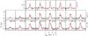 |
Fig. 1 DCO+ observations (histogram) and fit (red line) for J:1–0 (bottom line), J:2–1 (middle line), and J:3–2 (top line) across L183 main PSC. Offsets are indicated for the J:1–0 transition and apply to all. The cut, though sparcely sampled for the J:2–1 and J:3–2 lines, is along the same N2H+ cut as in Paper I and crosses the dust peak. |
Though CO is the main species used to reveal depletion, many others are known to deplete. Water is probably the first one to deplete when penetrating the clouds owing to its H-bond capability and consequently high sublimation temperature (but is also difficult to study). Other species, such as CS and SO, have been shown to deplete (e.g. Tafalla et al. 2002, 2004; Pagani et al. 2005). A controversy has arisen about the remarkable resistance of N-bearing species to not depleting and their column density to being, on first order, proportional to the amount of dust. Such is the case for NH3, CN, HCN, and N2H+. For NH3, Tafalla et al. (2002, 2004) even show an increase in abundance in the prestellar core centers, while N2H+ abundance seems to be constant with radius. The absence of depletion for CN and HCN has been reported by Hily-Blant et al. (2008, 2010). A few works indicate possible depletion of N2H+(Bergin et al. 2002; Belloche & André 2004; Di Francesco et al. 2004), and Pagani et al. (2007, hereafter Paper I) use a detailed radiative transfer modeling of L183 to show that N2H+ starts to decrease in abundance above n ≈ 5 × 105 cm-3, a possible sign of the depletion of its parent species N2 above that density. However, the reason for this late depletion of N2 compared to that of CO is not clear, since both species have the same weight, one is apolar, the other weakly polar, and therefore should have approximately comparable behaviors in terms of freezing-out and desorption mechanisms. Despite their similarity, chemical models have tried to reproduce the different behaviors of both species by supposing different binding energies (e.g. Bergin & Langer 1997; Bergin et al. 2002), but laboratory work has shown that this is not correct (Öberg et al. 2005; Bisschop et al. 2006; Öberg et al. 2009) so the problem persists. Because both DCO+ and the pair (N2H+, N2D+) are observed in depleted cores, one possible explanation is that CO and N2 both deplete in similar proportions, but since their relative abundances to H2 before depletion are very high (X[CO] = CO/H2 ≈ 1 × 10⁻⁴ and possibly X[N2] ≈ 1 × 10⁻⁵), enough molecules remain, even for a factor 1000 depletion, to produce these daughter species to their observed abundances (typically in the range 1 × 10-11–1 × 10⁻¹⁰). However, observations of N2 itself are impossible because of the lack of a dipole moment, which prevents emission in the radio domain, and CO emission in the core is masked by the strong CO lines emitted in the undepleted parts of the cloud. This is true for all CO isotopologues. Since CO is easily thermalized in clouds, even their envelope shines strongly in the low rotational transitions, and column density fluctuations (the envelope is certainly not a regular sphere of constant thickness) do not allow retrieval of the CO abundance inside the core. Another limitation comes from the finite signal-to-noise ratio of observed spectra. To detect a variation of 10% in intensity, a signal-to-noise ratio of 30 would be required and that would hardly be sufficient to separate an abundance drop of 100 from one of 103 (though such an attempt has been made recently, Brady-Ford & Shirley 2011, but the authors do conclude that they cannot distinguish between a depletion factor of 10 or of 1000).
Based on the fact that DCO+ is a daughter species of CO and that it is present almost only in the depleted core (unlike the other HCO+ isotopologues, see Pagani et al. 2011), we propose to retrieve the abundance profile of CO where it depletes. Measuring DCO+ alone would imply having to rely entirely on a chemical model to retrieve CO. Here, we propose to take advantage of the measurement of three other species, N2H+, N2D+, and H2D+, which are also confined to the prestellar core, to strongly constrain the deuteration enrichment process of DCO+ and therefore constrain the CO abundance itself. We simply have to exploit the model presented in Pagani et al. (2009, hereafter Paper II) and adjust it to explain all four observed species. The outcome is the N2 and CO abundance profiles across the core.
In Sect. 2, we present the DCO+ observations of one test case, the L183 prestellar core, and in Sect. 3 their radiative transfer modeling. Section 4 presents the method for constraining the CO and N2 abundances from the observations of daughter species. We discuss their depletion profiles in L183 and present our conclusions in Sect. 5. DCO+–H2 collisional rates are presented in Appendix A.
2. Observations
We observed DCO+ (J:1–0), (J:2–1), and (J:3–2)lines with the IRAM – 30 m from 12 to 14 July 2008. For the (J:1–0)transition, the image rejection was relatively low, the receiver being somewhat outside the original range of frequencies for which it was designed and close to the low side cutoff-frequency. Therefore the image/signal gain ratio was measured after the tuning and found to be 0.73. The other lines benefited from standard tunings with gain ratios of only 0.03. The sky was reasonably good. Zenithal opacity was 0.15, 0.1, and 0.3 for the (J:1–0), (J:2–1), and (J:3–2)lines, respectively and the system temperature of the order of 400, 200, and 450 K (in the  scale, similar to the
  scale for this telescope, see Pagani et al. 2005). We used the versatile autocorrelator as a backend (VESPA) with resolutions of 10, 10, and 40 kHz, respectively, corresponding to velocity resolutions of 41, 20, and 54 m s-1 with bandwidths of 40, 20, and 40 MHz. The spatial resolution is 36, 18, and 12′′, respectively. Observations were done in frequency-switch mode. The pointing and focus were checked. The pointing accuracy remained within 3′′.
The N2H+ and N2D+ observations were described and analyzed in Paper I, while the ortho-H2D+ data are presented and analyzed in Paper II. The reference position is α(2000) = 15h54m08.5s, δ(2000) = −2°52′48′′.
3. Analysis
For DCO+, we performed only two short perpendicular cuts: one vertical, along the dense filament, and one perpendicular to it, with 24′′ spacings. Only the horizontal cut is displayed in Fig. 1. As for N2H+, N2D+, and ortho-H2D+, the line intensities peak toward the prestellar core and are approximately constant along the ridge. They strongly decrease away from it to the left (east). The decrease is not as strong to the right (west) because a secondary dust peak lies slightly farther away in that direction (see Pagani et al. 2004). Due to its hyperfine structure (HFS, Caselli & Dore 2005), the (J:1–0) line is markedly wider (0.54 km s-1) than the (J:2–1) line (0.44 km s-1), itself wider than the (J:3–2) line (0.3 km s-1) and all of them being wider than the N2D+ and N2H+ lines (0.2 km s-1). Fitting the lines with the CLASS HFS routine loaded with the description of the DCO+ HFS structure, we found a velocity width of ~0.2 km s-1 for each HFS component, in agreement with the N2H+ and N2D+ determinations.
We modeled the DCO+ emission using the best-fit model of the L183 PSC in density, temperature, and large-scale velocity (see Paper I, their Table 2) and the same spherical Monte-Carlo radiative transfer model adapted to HFS treatment, including line overlap as for N2D+ and N2H+ (Paper I). Though recent HFS-resolved DCO+–He collisional coefficients have been published (Buffa 2012), we found that it was impossible to fit the observations with the same density and temperature profile as for N2H+, the modeled lines being far too weak. Instead, we computed new HFS-resolved DCO+–H2 rate coefficients based on those of HCO+ with para-H2 from BASECOL (Flower 1999; Dubernet et al. 2006), following the method proposed by Faure & Lique (2012, see Appendix). To compare the model to the observations, we convolved the model output as if it was coming from a cylinder (to mimic the filament) with the 30-m main beam and error beams (as in Paper I).The Monte-Carlo output fit is displayed in Fig. 1 and the resulting DCO+ abundance fit with its estimated dispersion is displayed in Fig. 2. The only free parameter of the model is the DCO+ abundance profile. The N2D+ abundance profile (from Paper I, Table 2) is traced in the same figure. While the N2D+ abundance shows only a mild diminution in the PSC center, DCO+ is clearly more extended than N2D+, but the central drop is a factor ≥ 17, almost one order of magnitude more than that of N2D+.
4. Description of the method
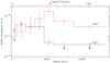 |
Fig. 2 DCO+ relative abundance (in volume) from the radiative transfer fit of the observations (in red). N2D+ abundance (from Paper I, Table 2) is also displayed. The x axis is cylindrical radius referring to Fig. 1. |
To determine CO abundance from DCO+ observations, one needs to know the main reaction paths that lead from CO to DCO+ and the main destruction routes of DCO+. Chemical models can perform such an analysis but they depend on initial conditions, some of which are difficult to know, such as the grain size distribution or the cosmic ray ionization rate. In the case of a depleted PSC, the main reactions that form DCO+ involve CO and the three deuterated H3+ isotopologues. With the possible measurement of only one or rarely two of these species, namely ortho-H2D+ and para-D2H+, too many solutions can be found with various CO abundances to fit the observed DCO+ abundance. To avoid these uncertainties, we instead consider the isotopologue ratio DCO+/HCO+. They both derive mostly from reactions of CO with H3+ isotopologues (in depleted cores) and are both destroyed by (mostly) electrons. Therefore the DCO+/HCO+ ratio only depends on the balance between the four H3+ isotopologues. CO and e− abundances are not needed to determine this balance. Therefore, knowing the abundance of one of the H3+ isotopologues and the balance between them, a unique solution of the deuteration enrichment can be found. We also need to know the destruction rate of DCO+ with the electrons to fix the CO abundance. The e− abundance depends primarily on the density and on the cosmic ray ionization rate (Walmsley et al. 2004). In Paper II, the cosmic ray ionization rate (and therefore the e− abundance) is not a free parameter (though not mentioned). We had to adjust it to both fit the deuteration balance and the ortho-H2D+ observed abundance at the same moment, and the range of possible values was relatively narrow (ζ = 2–3 × 10-17 s-1). Therefore the knowledge of the DCO+/HCO+ ratio and of the ortho-H2D+ abundance allows to constrain uniquely the CO abundance. However, the scheme is not feasible because HCO+ is spread all over the cloud since CO and H3+ are both abundant everywhere. Since the HCO+ lines are very optically thick, there is no possibility to derive the HCO+ abundance inside the PSC itself and the DCO+/HCO+ ratio cannot be established. H13CO+ meets the same problem, and HC18O+ is too weak here. Instead, because the DCO+/HCO+ and the N2D+/N2H+ ratios follow the same chemical scheme inside the PSC (Pagani et al. 2011), and both depend only on the same deuteration balance we use the latter ratio to determine that balance, since both its species are confined to the PSC.
Quantitatively, we ran the same chemical model as in Paper II, and we refer the reader to it for details. However, we slightly modified the reaction network. We introduced the new ortho–H2 + H+ ↔ para–H2 + H+ reaction rate from Honvault et al. (2011), which shows that this conversion rate is slowed by a factor of 2 compared to the previous value (Gerlich 1990). The effect is to slow down the ortho-to-para H2 conversion and somewhat increase the time it takes for deuteration processes to become efficient (see Paper II). Recombination of N2H+ with electrons is supposed to give only N2 + H and not N + NH (see however Hily-Blant et al. 2010, for a different approach and discussion therein). Because these reactions of formation and destruction of HCO+ and N2H+ are relatively fast (100 years, Parise et al. 2011), we consider that even if other phenomena compete for the CO or for the N2 ressources, like depletion, fitting the observed N2H+, N2D+, and DCO+ local abundances gives the present abundance of the parent molecule, N2 or CO. To find the CO abundance needed to explain the DCO+ abundance in the model, we adjust the CO one, until the DCO+ abundance reaches the observed value at the same moment as the observed N2D+/N2H+ ratio and ortho-H2D+ abundance are reached, layer after layer (see Paper II, their Fig. 7). Because N2H+ and N2D+ react with CO to form HCO+ and DCO+, respectively, the abundance of N2 slightly depends upon that of CO and needs to be adjusted after that of CO to reproduce the observed N2D+ and N2H+ abundances. If the edge of the depleted region is reached, we should be able to smoothly connect the CO abundance derived from our modeling with the undepleted CO abundance. However, N2D+ usually disappears before reaching this edge, thus preventing the model to be extended that far, and it is possible that abundance jumps exist (Pagani et al. 2010).
5. Discussion and conclusion
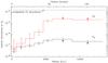 |
Fig. 3 CO and N2 relative abundances (in volume) derived from the chemical model. The x-axis is cylindrical radius referring to Fig. 1. |
Figure 3 shows the modeled CO and N2 abundance profiles in the PSC as a function of distance. Lower limits for CO in the outer parts are due to the upper limit on N2D+ abundance, limiting our knowledge of the H3+ isotopologue balance. The upper limit in the center is linked to the DCO+ upper limit itself. CO abundance starts close to the undepleted abundance (1–2 × 10⁻⁴, e.g., Dickman 1978; Pineda et al. 2010). It drops by ≥ 360 in the PSC and by ≥ 2000 compared to the undepleted abundance. This is the first time such a drop has been reported. It is possibly not unique to this source, but this question will be addressed when we have extended this method to other PSCs. It is interesting to note that the CO profile compares favorably with the results of Aikawa et al. (2005), especially their case with a peak density of 3 × 106 cm-3, and α = 4 (=fast collapse case, their Fig. 3, middle left) which is close to the L183 PSC conditions.
The N2 abundance seems to first increase up to ≤ 3.7 × 10⁻⁷, much lower than what it would reach in a chemical model at steady state (~1 × 10⁻⁵, Flower et al. 2006) but then decreases only by a factor of ≤ 12. This is also the first time that such a profile can be reported and that the CO and N2 profiles are compared. From the work of Öberg et al. (2005, 2009) and Bisschop et al. (2006), we know that this different behavior cannot be attributed to different adsorption and desorption properties of both species. Because N2 has not reached its steady state abundance, contrary to CO, it is possible that enough atomic N is still available to keep forming N2 in the core. Di Francesco et al. (2007) indicate that atomic N has a lower binding energy than N2 or CO, which would help in this scenario. A possible route to the formation of N2 from N involves the presence of CN (e.g., Hily-Blant et al. 2010):  (1)Hily-Blant et al. (2008) have shown that CN is not depleted in L183, with an abundance of ~8 × 10⁻¹⁰. The production rate of N2 (k × [N] [CN] , with k ~ 5 × 10-11 cm3 s-1, Wakelam et al. 2012, and [N] and [CN] the density of the species) would therefore be 1.6 × 10⁻⁷ X[N] cm-3 s-1 in the center of the PSC (where n(H2) = 2 × 106 cm-3) down to 4.6 × 10⁻¹¹ X[N] cm-3 s-1 at the edge (n(H2) = 3.4 × 104 cm-3), to be compared to the freeze-out rate (e.g., Bergin & Tafalla 2007), [N2]kfo = 2.6 × 10⁻⁵ X[N2] cm-3 s-1 at the center and 7.5 × 10⁻⁹ X[N2] cm-3 s-1 at the edge. For the X[N2] values found here, we see that though the depletion rate is low at the edge (1.5 × 10⁻¹⁵ cm-3 s-1), the formation rate cannot compensate for any reasonable value of X[N] (4.6 × 10⁻¹⁶ cm-3 s-1 for X[N] = 1 × 10⁻⁵). In the center, the depletion rate is much higher (8 × 10-13 cm-3 s-1), but the N2 production rate is in the range 1.8 × 10⁻¹²–10-14 for X[N] = 1 × 10⁻⁵–10-7), and therefore comparable. If N is not too depleted in PSCs, combined to the presence of CN, this could explain the slower decrease in N2 with density than in CO.
The method presented here suffers from two types of uncertainties: on collisional coefficients and on reaction rates. The critical ones are the N2H+–He collisional coefficients (Daniel et al. 2005) that underestimate the real N2H+–H2 ones and the ortho-H2D+–H2 collisional coefficients that are needed to
retrieve the ortho-H2D+ abundance (from Hugo et al. 2009). Therefore, the abundance profiles of DCO+, N2D+ (both depending on the temperature and density profiles derived from N2H+), and ortho-H2D+ remain tentative and were presented mostly to illustrate the method until new collisional coefficients become available. Less important, because the deuteration is constrained by the N2D+/N2H+ ratio, are the reaction rates of the H3+ network (evaluated statistically by Hugo et al. 2009).
The simple approach we propose here allows deriving the CO and N2 abundances in PSCs and tracing their profile without any strong dependence upon the initial conditions and with good precision, though it is still limited at the moment by uncertain coefficients and rates. The obtention of these profiles will allow several pending problems to be addressed such as the determination of the efficient processes to desorb molecules in PSCs, time-evolution of PSCs based on their depletion profiles and the CO/N2 differential depletion crisis.
Online material
Appendix A: DCO+–H2 collisional coefficients
Hyperfine-resolved DCO+–He rate coefficients have been published recently by Buffa (2012). It is generally assumed that rate coefficients with He multiplied by a factor of 1.4 can provide an estimate of rate coefficients with H2(J = 0) (Lique et al. 2008). However, for a molecular ion like DCO+, this approximation may be invalid, since the electrostatic interaction of an ion with H2 differs significantly from that with He. We have thus decided to determine hyperfine DCO+–H2 rate coefficients from close coupling (CC) HCO+–H2 rate coefficients ( ) of Flower (1999) using the Infinite order sudden (IOS) approximation described in Faure & Lique (2012). Here, the isotopic substitution of HCO+ has been ignored since it is expected to have a little impact on the magnitude of the rate coefficients (Buffa 2012).
In DCO+, the coupling between the nuclear spin (I = 1) of the deuterium atom and the molecular rotation results in a weak splitting (Alexander & Dagdigian 1985) of each rotational level J, into three hyperfine levels (except for the J = 0 level which is split into only 1 level). Each hyperfine level is designated by a quantum number F (F = I + J) varying between |I − J| and I + J.
Within the IOS approximation, inelastic rotational rate coefficients  can be calculated from the “fundamental” rates (those out of the lowest J = 0 level) as follows (e.g. Corey & McCourt 1983):
 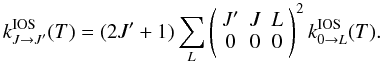 (A.1)Similarly, IOS rate coefficients among hyperfine structure levels can be obtained from the
  rate coefficients using the following formula (e.g. Corey & McCourt 1983):
 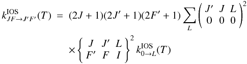 (A.2)
(A.2)
where  and { } are respectively the “3 − j” and “6 − j” Wigner symbols.
The IOS approximation is expected to be inaccurate at low temperature. However, it is also expected to correctly predict the relative rates among hyperfine levels within a rotational J → J′ transition. Propensity rules are indeed properly included through the Wigner coefficients. As a result, Neufeld & Green (1994) have suggested to compute the hyperfine rates as 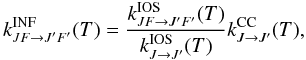 (A.3)using the CC rate coefficients kCC(0 → L) of Flower (1999) for the IOS “fundamental” rates () in Eqs. (A.1) and (A.2).
In addition, the fundamental excitation rates  were replaced by the fundamental de-excitation rates using the detailed balance relation:
 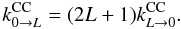 (A.4)This procedure is found to significantly improve the results at low temperature due to important threshold effects.
Then, from the HCO+–H2 rotational rate coefficients of Flower (1999), we have determined the IOS DCO+–H2 hyperfine rate coefficients using the computational scheme described above. The complete set of (de-)excitation rate coefficients is available online from the LAMDA1 and BASECOL2 websites.The present approach has been shown to be accurate, even at low temperature, and has also been shown to induce almost no consequence on the radiative transfer modeling compared to a more exact calculation of the DCO+–H2 rate coefficients (Faure & Lique 2012). However, we note that with the present approach, some hyperfine rate coefficients (those from the J = 1,F = 0 level to a J = F level) are strictly zero. This selection rule is explained by the “3 − j” and “6 − j” Wigner symbols that vanish for these kinds of transitions. Using a more accurate approach, these rate coefficients will not be strictly zero but will generally be smaller than the other rates. In addition, Faure & Lique (2012) have shown that it should imply almost no consequences for astrophysical modeling.
BASECOL: http://basecol.obspm.fr/
Acknowledgments
We are grateful to F. Daniel for providing us with the frequencies and Aijs of the DCO+ HFS, to P. F. Goldsmith for useful references, and to an anonymous referee who helped us to clarify and improve the manuscript.
References
- Aikawa, Y., Herbst, E., Roberts, H., & Caselli, P. 2005, ApJ, 620, 330 [NASA ADS] [CrossRef] [Google Scholar]
- Alexander, M. H., & Dagdigian, P. J. 1985, J. Chem. Phys., 83, 2191 [NASA ADS] [CrossRef] [Google Scholar]
- Belloche, A., & André, P. 2004, A&A, 419, L35 [NASA ADS] [CrossRef] [EDP Sciences] [Google Scholar]
- Bergin, E. A., & Langer, W. D. 1997, ApJ, 486, 316 [NASA ADS] [CrossRef] [Google Scholar]
- Bergin, E. A., & Tafalla, M. 2007, ARA&A, 45, 339 [NASA ADS] [CrossRef] [Google Scholar]
- Bergin, E. A., Alves, J., Huard, T., & Lada, C. J. 2002, ApJ, 570, L101 [NASA ADS] [CrossRef] [Google Scholar]
- Bisschop, S. E., Fraser, H. J., Öberg, K. I., et al. 2006, A&A, 449, 1297 [NASA ADS] [CrossRef] [EDP Sciences] [Google Scholar]
- Brady-Ford, A., & Shirley, Y. L. 2011, ApJ, 728, 144 [NASA ADS] [CrossRef] [Google Scholar]
- Buffa, G. 2012, MNRAS, 421, 719 [NASA ADS] [Google Scholar]
- Caselli, P., & Dore, L. 2005, A&A, 433, 1145 [NASA ADS] [CrossRef] [EDP Sciences] [Google Scholar]
- Caselli, P., Walmsley, C. M., et al. 1999, ApJ, 523, L165 [NASA ADS] [CrossRef] [Google Scholar]
- Corey, G. C., & McCourt, F. R. 1983, J. Phys. Chem., 87, 2723 [CrossRef] [Google Scholar]
- Daniel, F., Dubernet, M.-L., Meuwly, M., et al. 2005, MNRAS, 363, 1083 [NASA ADS] [CrossRef] [Google Scholar]
- Di Francesco, J., André, P., & Myers, P. C. 2004, ApJ, 617, 425 [NASA ADS] [CrossRef] [Google Scholar]
- Di Francesco, J., Evans II, N. J., et al. 2007, Protostars and Planets V, 17 [Google Scholar]
- Dickman, R. L. 1978, ApJS, 37, 407 [NASA ADS] [CrossRef] [Google Scholar]
- Dubernet, M.-L., et al. 2006, J. Plasma Res. Ser., 7, 356 [Google Scholar]
- Faure, A., & Lique, F. 2012, MNRAS, 425, 740 [Google Scholar]
- Flower, D. R. 1999, MNRAS, 305, 651 [NASA ADS] [CrossRef] [Google Scholar]
- Flower, D. R., Pineau Des Forêts, G., & Walmsley, C. M. 2006, A&A, 456, 215 [NASA ADS] [CrossRef] [EDP Sciences] [Google Scholar]
- Gerlich, D. 1990, JCP, 92, 2377 [Google Scholar]
- Herbst, E., & Klemperer, W. 1973, ApJ, 185, 505 [NASA ADS] [CrossRef] [Google Scholar]
- Hily-Blant, P., Walmsley, M., et al. 2008, A&A, 480, L5 [NASA ADS] [CrossRef] [EDP Sciences] [Google Scholar]
- Hily-Blant, P., Walmsley, M., et al. 2010, A&A, 513, A41 [NASA ADS] [CrossRef] [EDP Sciences] [Google Scholar]
- Honvault, P., Jorfi, M., et al. 2011, Phys. Chem. Chem. Phys., 131, 19089 [CrossRef] [Google Scholar]
- Hugo, E., Asvany, O., & Schlemmer, S. 2009, JCP, 130, 164302 [Google Scholar]
- Keto, E., & Caselli, P. 2008, ApJ, 683, 238 [NASA ADS] [CrossRef] [Google Scholar]
- Lemme, C., Walmsley, C. M., et al. 1995, A&A, 302, 509 [NASA ADS] [Google Scholar]
- Lique, F., Toboła, R., Kłos, J., et al. 2008, A&A, 478, 567 [NASA ADS] [CrossRef] [EDP Sciences] [Google Scholar]
- Neufeld, D. A., & Green, S. 1994, ApJ, 432, 158 [NASA ADS] [CrossRef] [Google Scholar]
- Öberg, K. I., van Broekhuizen, F., Fraser, H. J., et al. 2005, ApJ, 621, L33 [NASA ADS] [CrossRef] [Google Scholar]
- Öberg, K. I., van Dishoeck, E. F., & Linnartz, H. 2009, A&A, 496, 281 [NASA ADS] [CrossRef] [EDP Sciences] [Google Scholar]
- Pagani, L., Bacmann, A., Motte, F., et al. 2004, A&A, 417, 605 [NASA ADS] [CrossRef] [EDP Sciences] [Google Scholar]
- Pagani, L., Pardo, J.-R., Apponi, A. J., et al. 2005, A&A, 429, 181 [NASA ADS] [CrossRef] [EDP Sciences] [Google Scholar]
- Pagani, L., Bacmann, A., Cabrit, S., & Vastel, C. 2007, A&A, 467, 179 (Paper I) [NASA ADS] [CrossRef] [EDP Sciences] [Google Scholar]
- Pagani, L., Vastel, C., Hugo, E., et al. 2009, A&A, 494, 623 (Paper II) [NASA ADS] [CrossRef] [EDP Sciences] [Google Scholar]
- Pagani, L., Ristorcelli, I., Boudet, N., et al. 2010, A&A, 512, A3 [Google Scholar]
- Pagani, L., Roueff, E., & Lesaffre, P. 2011, ApJ, 739, L35 [NASA ADS] [CrossRef] [Google Scholar]
- Parise, B., Belloche, A., Du, F., et al. 2011, A&A, 526, A31 [NASA ADS] [CrossRef] [EDP Sciences] [Google Scholar]
- Pineda, J. L., Goldsmith, P. F., Chapman, N., et al. 2010, ApJ, 721, 686 [NASA ADS] [CrossRef] [Google Scholar]
- Tafalla, M., & Santiago, J. 2004, A&A, 414, L53 [Google Scholar]
- Tafalla, M., Myers, P. C., Caselli, P., et al. 2002, ApJ, 569, 815 [NASA ADS] [CrossRef] [Google Scholar]
- Tafalla, M., Myers, P. C., Caselli, P., & Walmsley, M. 2004, A&A, 416, 191 [NASA ADS] [CrossRef] [EDP Sciences] [Google Scholar]
- Wakelam, V., Herbst, E., Loison, J.-C., et al. 2012, ApJS, 199, 21 [NASA ADS] [CrossRef] [Google Scholar]
- Walmsley, C. M., Flower, D. R., & Pineau des Forêts, G. 2004, A&A, 418, 1035 [NASA ADS] [CrossRef] [EDP Sciences] [Google Scholar]
- Ward-Thompson, D., Scott, P. F., et al. 1994, MNRAS, 268, 276 [NASA ADS] [CrossRef] [Google Scholar]
- Willacy, K., Langer, W. D., & Velusamy, T. 1998, ApJ, 507, L171 [NASA ADS] [CrossRef] [Google Scholar]
All Figures
|
Fig. 1 DCO+ observations (histogram) and fit (red line) for J:1–0 (bottom line), J:2–1 (middle line), and J:3–2 (top line) across L183 main PSC. Offsets are indicated for the J:1–0 transition and apply to all. The cut, though sparcely sampled for the J:2–1 and J:3–2 lines, is along the same N2H+ cut as in Paper I and crosses the dust peak. |
| In the text | |
|
Fig. 2 DCO+ relative abundance (in volume) from the radiative transfer fit of the observations (in red). N2D+ abundance (from Paper I, Table 2) is also displayed. The x axis is cylindrical radius referring to Fig. 1. |
| In the text | |
|
Fig. 3 CO and N2 relative abundances (in volume) derived from the chemical model. The x-axis is cylindrical radius referring to Fig. 1. |
| In the text | |
Current usage metrics show cumulative count of Article Views (full-text article views including HTML views, PDF and ePub downloads, according to the available data) and Abstracts Views on Vision4Press platform.
Data correspond to usage on the plateform after 2015. The current usage metrics is available 48-96 hours after online publication and is updated daily on week days.
Initial download of the metrics may take a while.