| Issue |
A&A
Volume 548, December 2012
|
|
|---|---|---|
| Article Number | A45 | |
| Number of page(s) | 19 | |
| Section | Extragalactic astronomy | |
| DOI | https://doi.org/10.1051/0004-6361/201220059 | |
| Published online | 19 November 2012 | |
Jet and torus orientations in high redshift radio galaxies⋆
1
European Southern Observatory,
Karl Schwarzschild Straße 2,
85748
Garching bei München,
Germany
e-mail: This email address is being protected from spambots. You need JavaScript enabled to view it.
2
Institut d’Astrophysique de Paris, 98bis boulevard Arago, 75014
Paris,
France
3
CSIRO Astronomy & Space Science, PO Box
76, Epping,
NSW
1710,
Australia
4
Jet Propulsion Laboratory, California Institute of
Technology, Mail Stop
169-221, Pasadena,
CA
91109,
USA
5
Astronomisches Institut, Ruhr-Universität Bochum, Universitätstr.
150, 44801
Bochum,
Germany
6
Oceanit Laboratories, 828 Fort Street Mall, Suite 600, Honolulu, HI
96813,
USA
Received: 19 July 2012
Accepted: 19 September 2012
Abstract
We examine the relative orientation of radio jets and dusty tori surrounding the active galactic nucleus (AGN) in powerful radio galaxies at z > 1. The radio core dominance  serves as an orientation indicator, measuring the ratio between the anisotropic Doppler-beamed core emission and the isotropic lobe emission. Assuming a fixed cylindrical geometry for the hot, dusty torus, we derive its inclination i by fitting optically-thick radiative transfer models to spectral energy distributions obtained with the Spitzer Space Telescope. We find a highly significant anti-correlation (p < 0.0001) between R and i in our sample of 35 type 2 AGN combined with a sample of 18 z ~ 1 3CR sources containing both type 1 and 2 AGN. This analysis provides observational evidence both for the Unified scheme of AGN and for the common assumption that radio jets are in general perpendicular to the plane of the torus. The use of inclinations derived from mid-infrared photometry breaks several degeneracies which have been problematic in earlier analyses. We illustrate this by deriving the core Lorentz factor Γ from the R-i anti-correlation, finding Γ ≳ 1.3.
Key words: galaxies: high-redshift / galaxies: active / radio continuum: galaxies / infrared: galaxies / galaxies: jets / quasars: general
Figures 11, 12, and Tables 1, 2, 6 are available in electronic form at http://www.aanda.org
© ESO, 2012
1. Introduction
Radio galaxies are among the most luminous objects in the Universe over the entire electromagnetic spectrum. Their powerful radio emission betrays the presence of a central massive black hole (Blandford & Payne 1982) up to a few billion M⊙ in mass (McLure et al. 2006; Nesvadba et al. 2011). Early in the development of the subject, local radio galaxies were associated with massive elliptical galaxies (Matthews et al. 1964). It is now well established that powerful radio sources are also hosted by massive galaxies at higher redshift (e.g. De Breuck et al. 2010), as expected from the bulge-black hole mass relation (Ferrarese & Merritt 2000). Radio galaxies appear to be a singular stage in the evolution of massive galaxies, observed during a peak of activity. This phase presents a unique chance to test models of galaxy formation and the interaction between the AGN and their host galaxies (e.g. Nesvadba et al. 2008).
According to current understanding, an active galactic nucleus (AGN) consists of an accretion disk around a supermassive black hole (SMBH; Rees 1984). About 10% of AGN show radio jets (e.g. Best et al. 2005); these are expected to be aligned with the black hole spin axis. A dusty torus has been hypothesized to explain the observed dichotomy between unobscured (type 1) AGN where the observer can see the region close to the black hole directly and obscured (type 2) AGN with a more edge-on view (for a review, see Antonucci 1993). As a result of this geometry, the AGN emission is anisotropic at most wavelengths. The accretion disk is a powerful source of soft and hard X-rays which are attenuated when passing through the torus. Assuming a universal torus shape, the dominating factor determining the amount of obscuration along the line of sight is the orientation of the torus with respect to the observer. In particular, soft X-rays are sensitive to the hydrogen column density (NH) which varies from 1020 cm-2 in type 1 AGN to > 1024 cm-2 type 2 AGN (e.g. Ibar & Lira 2007).
In the optical domain, the effects of inclination can explain why the Broad Line Regions (BLR) are observed directly in type 1 AGN, while in type 2’s, they are mostly obscured or seen in scattered emission (Antonucci & Miller 1985; Tran et al. 1992). In both types, Narrow Line Regions (NLR) are observed further out from the torus. In the case of type 2’s, the torus acts as a coronograph blocking the much brighter central emission, and allows the NLR to be traced out to ~100 kpc (Reuland et al. 2003; Villar-Martín et al. 2003). Such detailed studies have shown that the NLR is frequently aligned with the radio jets (McCarthy et al. 1987). Moreover, optical polarimetry of type 2 AGN reveals a continuum polarization angle mostly perpendicular to the radio axis, implying that the light passing through torus opening is scattered by dust clouds along the radio jets (di Serego Alighieri et al. 1989, 1993; Cimatti et al. 1993; Hines 1994; Vernet et al. 2001). Both observations imply that the radio jets are aligned orthogonally to the equatorial plane of the torus.
The torus surrounding the SMBH re-processes a significant fraction of the AGN radiation (X-rays, UV and optical) into mid-IR thermal dust emission. This establishes a radial temperature gradient within the torus ranging from the sublimation temperature (~1500 K) at the inner surface of the torus to a few hundred Kelvin in the outer parts. The torus geometry creates a strong anisotropy in the hot dust emission because the amount of extinction towards the innermost (hottest) parts is very sensitive to the orientation with respect to the observer (Pier & Krolik 1992,hereafter PK92). It should therefore be possible to derive the inclination by modelling of the mid-IR SED. The magnitude of the variation with inclination is illustrated by the difference between the mean type 1 and type 2 mid-IR SEDs of an isotropically selected AGN sample where the type 2 AGN SED can be reproduced by simple reddening of the type 1 distribution (Haas et al. 2008).
The most isotropic emission from AGN comes from the radio lobes which mark the interaction between the jets and the surrounding intergalactic medium. This can happen on scales as large as several Mpc and produces steep-spectrum synchrotron emission. In contrast, the radio cores generally have flatter spectral indices and are anisotropic as they are subject to Doppler beaming effects. The radio cores will look brighter if the jet axis is observed closer to the line of sight (e.g. in type 1 AGN). The ratio of the core to total radio emission (core dominance) is a proxy for orientation (e.g. Scheuer & Readhead 1979; Kapahi & Saikia 1982).
In summary, previous observations suggest that the radio jets are orthogonal to the equatorial plane of the torus. Assuming a generic torus geometry, an inclination can be derived by fitting the mid-IR SED; the core dominance can also be used to estimate the inclination of the radio jets. Provided that these assumptions are correct, the two measures of inclination should be consistent. In this paper, we make use of the unique database consisting of six-band mid-IR data for 70 radio galaxies spanning z = 1 to z = 5.2 (Seymour et al. 2007; De Breuck et al. 2010, S07 and DB10 hereafter). We derive the inclination angle by fitting dust emission from the torus, and compare it with the radio core dominance. We indeed find a significant correlation between these parameters, consistent with the previously mentioned observational statements which sample directions in the plane of the sky. We also use this constraint on the orientation to estimate the pc-scale jet speeds from the core/jet dominance.
This paper is organised as follows. Sections 2 and 3 describe the samples. In Sect. 4, we describe our approach to modelling the mid-IR emission, using both empirical correlations and a torus model for a sub-sample with well-sampled AGN dust emission. We discuss the implications in Sect. 5. Throughout this paper, we adopt the current standard cosmological model (H0 = 70 km s-1 Mpc-1, ΩΛ = 0.7, ΩM = 0.3).
2. Spitzer high redshift radio galaxy sample
Our Spitzer high redshift radio galaxy (SHzRG) sample is selected from a compendium of the most powerful radio galaxies known in 2002. From this parent sample of 225 HzRGs with spectroscopic redshifts, a subset was selected in order to sample the redshift-radio power plane evenly out to the highest redshifts available. The full description of this sample is presented by S07. In short, the HzRG are distributed across 1 < z < 5.2 and have P3 GHz > 1026 W Hz-1, where P3 GHz is the total luminosity at a rest-frame frequency of 3 GHz (Table 1 of S07).
2.1. Infrared data
The mid-IR data presented here were obtained with the Spitzer Space Telescope (Werner et al. 2004) during Cycles 1 and 4. All galaxies were observed in the four Infrared Array Camera (IRAC; Fazio et al. 2004) channels (3.6, 4.5, 5.8, 8 μm), the 16 μm peak-up mode of the Infrared Spectrograph (IRS; Houck et al. 2004) and the 24 μm channel of the Multiband Infared Photometer (MIPS; Rieke et al. 2004). The 24 sources with the lowest expected background emission were also observed with the 70 and 160 μm channels of MIPS. We refer the reader to S07 and DB10 for the full description of the data reduction procedures and the full photometric data (Table 3 of DB10). We augment our photometry with K-band magnitudes from S07.
2.2. Radio data and core dominance
The radio morphologies of HzRGs are dominated by steep-spectrum radio lobes with fainter and flatter spectrum radio cores (Carilli et al. 1997; Pentericci et al. 2000). A variety of physical processes contribute to the radio emission at different restframe frequencies (e.g. Blundell et al. 1999). Above ν ≈ 1 GHz, Doppler boosting will introduce an orientation bias in the radio cores. In addition, the radio lobes are affected by synchrotron and inverse Compton losses. At very low frequencies ν ≲ 100 MHz, synchrotron self-absorption, free-free absorption and any low-energy cutoff of the relativistic particles may reduce the observed synchrotron emission. We therefore choose a rest-frame wavelength of 500 MHz to obtain an accurate measure of the energy injected by the AGN which is also independent of orientation. Observationally, the 500 MHz luminosities  can also be determined most uniformly over the entire sky (DB10).
Our measure of orientation for the radio jets is the ratio of core to extended emission or core dominance R (Scheuer & Readhead 1979; Kapahi & Saikia 1982). Since the flatter spectrum cores can only be spatially resolved with interferometers at high frequencies, this is defined as  , where
  is the 20 GHz restframe core luminosity.
Core flux densities are either taken from the literature (see Table 1), or measured directly from radio maps by the following method. First, we take the Spitzer/IRAC 3.6 μm image and overlay the radio contours. After identifying the core with the host galaxy, we measure the integrated total and core flux densities using the aips verb tvstat. If only the lobes are identified, we derive an upper limit to the core dominance from the 3σ sensitivity of the radio map. Next, we calculate  using 8.4 GHz observations and the core spectral index αcore, defined as S ∝ να. If no spectral index is available, we use the median value from our sample ⟨ αcore ⟩ = −0.8. Note that given the large range of R, the exact value of αcore does not significantly affect our results. At higher redshifts, inverse Compton losses can increase significantly, which may affect R values. However, Fig. 1 does not show a significant dependence of R on redshift, so we consider this effect to be negligible.
Table 1 lists the values of  (summing the components in the case of multiple detections) and R, together with the core flux densities and spectral indices αcore (see references in Table 1).
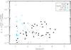 |
Fig. 1 Core dominance R versus redshift. Note the lower redshifts for the s3CR sample (blue diamonds and open squares). The open black diamonds correspond to radio galaxies with observed broad lines, see Sect. 5.3. |
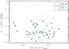 |
Fig. 2 Core dominance R versus |

3. 3CR sample
To compare the results of our approach for type 1 and 2 radio-loud AGN, samples of the two classes with matched selection criteria are required. Unfortunately, there is no type 1 (quasar) sample in the literature which matches our radio-galaxy sample and has both radio and Spitzer observations. The best sample available, although significantly smaller than our SHzRG sample and with a lower median redshift, is the 3CR sample (Spinrad et al. 1985).
3.1. Infrared data
A selection of 64 3CR high-redshift sources has been observed with the four IRAC channels (3.6, 4.5, 5.8, 8 μm), IRS (16 μm) and the MIPS1 channel (24 μm). We refer to Haas et al. (2008) for a full description of the sample and data reduction. Table 2 reports the Spitzer photometry.
3.2. Radio data and core dominance
To compare the 3CR and SHzRG sources, we need equivalent radio data for both groups. We take the relevant measurements for the subset of 3CR sources from Hoekstra et al. (1997). Selecting sources with both Spitzer and radio data gives us a subset of 18 sources: 11 quasars and 7 radio galaxies. The radio data are reported in Table 3. We recalculate the 500 MHz rest-frame luminosity from the 178 MHz flux densities (Hoekstra et al. 1997, and references therein), using a spectral index α = −1.5, which is typical of powerful steep-spectrum radio sources in this frequency range. The 20 GHz rest-frame core luminosities are calculated using the flux density at 5 GHz assuming αcore = −0.8. The derived values of R are also reported in Table 3.
Radio data for the s3CR sample.
4. Modelling the torus emission
4.1. Contributions to the infrared SED
The near- to far-IR emission from radio galaxies and quasars consists of several components: (i) non-thermal synchrotron emission; (ii) line emission; (iii) starburst- and AGN-heated dust continuum; (iv) an (old) stellar population. We now discuss the importance of these contributions in turn.
Of the type 2 objects in our sample, the source which is likely to have the highest synchrotron contribution at 5 μm wavelength is B3 J2330+3927, which has the highest value of R and one of the flattest core spectra (α = −0.1). Its extrapolated synchrotron contribution is <5% of the total emission at 5 μm. The synchrotron contribution can therefore be safely ignored for all of the type 2 objects. However in type 1 objects, this assumption may not be valid. We further discuss this point in Sect. 5.2.2.
The line emission is dominated by fine structure and CO lines in the far-IR (e.g. Smail et al. 2011), and in the mid-IR by polycyclic aromatic hydrocarbon (PAH) emission. The silicate emission/absorption is also seen in type 1/2 AGN, respectively. Both can affect the broad-band photometry. Due to the large redshift range of our sources, the sampling of the SED differs from object to object. To keep our study as homogeneous as possible, we focus only on the part of the SED below the silicate feature (<10 μm), which is dominated by AGN heated dust emission (see below). Mid-IR spectroscopy with IRS (Seymour et al. 2008; Leipski et al. 2010; Rawlings et al., in prep.) shows that PAH features are either not detected or weak relative to the AGN emission.
The contribution of the dust continuum spans three orders of magnitude in wavelength. The energy source of this emission (AGN and/or starburst) has been the subject of considerable debate (e.g. Sanders et al. 1988; Haas et al. 2003). To disentangle these two components, good sampling of the entire IR SED is essential. The Herschel Radio Galaxy Evolution or projet HeRGÉ will observe our sample between 70 μm and 500 μm. First results on PKS1138−262 (Seymour et al. 2012) show that the AGN component dominates for λrest ≲ 30 μm. The contribution of starburst-heated dust may vary from source to source, but is unlikely to contribute significantly at λrest ≲ 10 μm as the required dust temperature would be more than several hundred Kelvin, which cannot be sustained throughout the host galaxy. We consequently focus only on λrest ≲ 10 μm. A crucial ingredient in modelling the torus is the 9.7 μm silicate feature, which can be used as an indicator of its intrinsic properties (e.g. the differences between clumpy and continuous or optically thin and thick tori and the dust composition; van Bemmel & Dullemond 2003). Using this feature to characterize the torus is beyond the scope of this paper, since our broad-band photometry is not particularly sensitive to it.
Emission from the old stellar population peaks at λrest ~ 1.6 μm (S07). In this paper, we model this contribution assuming a formation redshift zform = 10, using an elliptical-galaxy template predicted by PEGASE.2 (Fioc & Rocca-Volmerange 1997). The stellar contribution from this galaxy template is then normalised for the bluest available band and subtracted in each filter. Uncertainties for the subtracted data are taken to be the rms of the uncertainties of the individual measurement and the stellar fit. For the type 2 3CR radio galaxies, we follow the same method. For the type 1 3CR AGN, we do not subtract any stellar contribution, as the transmitted non-thermal continuum is expected to dominate over the stellar emission. The remaining flux is considered to be a “pure” AGN contribution.
4.2. Sub-samples with well-sampled AGN dust emission
After stellar subtraction (see Sect. 4.1), the signal to noise ratio (S/N) is calculated for each data-point. Then, we create a preferred sub-sample fulfilling the criteria that: (a) there are at least 3 points with S/N > 2; and (b) there is no significant contribution from emission with λrest > 10 μm in the passband. This in practice restricts the wavelength range to 2 μm <λrest < 8 μm in any passband. 35 radio galaxies from the SHzRG sample and 50 sources (22 radio galaxies, 25 quasars and 3 unidentified) from the 3CR sample meet these criteria. We refer to these two restricted samples as “sSHzRG” and “s3CR” respectively. Note that only 31 objects have a known core dominance value in sSHzRG and 18 in the s3CR (11 quasars and 7 radio galaxies).
4.3. Empirical approach
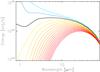 |
Fig. 3 Template SEDs for the empirical approach. The black curve is the mean quasar spectrum from Richards et al. (2006). The bluer/redder curves correspond to a increasing extinction (from –12 to 90 Av in steps of 6), using the Fitzpatrick (1999) extinction law. |
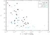 |
Fig. 4 Extinction AV versus core dominance R. Note the absence of points in the top right part of the plot. This figure is consistent with Fig. 12 of Cleary et al. (2007). |
To first order, increasing the viewing angle of the torus causes it to act as a varying dust screen: higher inclinations lead to increased extinction of the hottest dust located in the innermost parts of the torus. Leipski et al. (2010) and Haas et al. (2008) have shown that the mean radio galaxy SED can be approximated by applying an extinction law to the mean quasar SED.
Following the same approach, we model this dust absorption using the mean Sloan Digital Sky Survey (SDSS) quasar spectrum (Richards et al. 2006) and a Fitzpatrick (1999) extinction law with classical Galactic dust properties (RV = 3.1, Fig. 3). This law extrapolates Galactic dust properties to the mid-IR without any specific treatment of the silicate absorption and emission features around 10 μm. This latter approximation is still valid as we are focusing on the 2–8 μm part of the SED.
Using a standard χ2 minimization technique, we fit two parameters (extinction AV and normalization) to the data for our sSHzRG and s3CR samples. Tables 5 and 6 report the resulting values of AV. Figure 4 plots AV against R for the subset of objects with radio data available. Note the apparently unphysical negative AV values for the majority of s3CR quasars, which are bluer than the composite SDSS template. The lack of points in the upper right part of this plot indicates an absence of core-dominated objects with high extinction, as expected from the orientation-based Unified model (e.g. Antonucci 1993).
To test the correlation between AV and core dominance taking the upper limits in R into account, we use the survival analysis package within IRAF. The generalized Spearman rank test gives probabilities of non-correlation of p = 0.009 and p = 0.0001 for sSHzRG and sSHzRG+s3CR samples, respectively. We note that Cleary et al. (2007) report a similar distribution (their Fig. 12), although with a different core dominance definition and using the silicate optical depth, τ9.7 μm as a mesure of extinction.
4.4. Torus models
We now aim to reproduce the observed range in extinction assuming a torus geometry observed at varying angles to the line of sight. The infrared torus SED has been modelled extensively, assuming structures with various degrees of complexity. Despite the evidence for a clumpy structure (Krolik & Begelman 1988), the first models to solve the radiative transfer equations used the continuous density approximation (Pier & Krolik 1992). Later, a treatment of the clumpy structure was given by Nenkova et al. (2002). Currently, models with continuous and clumpy structures are available in the literature with a range of geometries and using different computational techniques to solve the radiative transfer equation. Examples include: continuous models (Pier & Krolik 1992; Dullemond & van Bemmel 2005; Granato & Danese 1994; Rowan-Robinson 1995); clumpy models (van Bemmel & Dullemond 2003; Hönig et al. 2006; Schartmann et al. 2005; Fritz et al. 2006; Nenkova et al. 2008) and bi-phased models (Stalevski et al. 2012).
Clumpy models are closer to reality than continuous models, but the latter require fewer free parameters and remain valid if the inter-clump distance is not significantly larger than the clump size. While more sophisticated modelling may be possible for some individual objects, our aim is to extract global trends from as many sources as possible in our sample. Because of the small number and irregular sampling of the data points in the mid-IR, we therefore opt for the Pier & Krolik continuous model (PK model, hereafter). Trying to derive detailed information on the torus itself is beyond the scope of this paper, and remains challenging even at lower redshift (e.g. Ramos Almeida et al. 2009; Kishimoto et al. 2011).
The PK model assumes a cylindrical geometry for the torus. The opening angle of the torus is θ = tan-1(2a/h), where a/h is the aspect ratio (Fig. 5). It models the spectrum of radiation from the central point sources as a power law decreasing from UV to IR. As the index of this power-law α does not have a significant effect for our purpose, we take the default value α = 1. We adopt an effective temperature for the inner edge of the torus of Teff = 1000 K as this is the only temperature available for all the geometries in the template library from PK92 (see Table 4). Indeed, a higher Teff corresponds to a higher contribution from the hottest dust (i.e. 1–2 μm) but would not affect the global analysis presented here.
The inner radius a (see Fig. 5) is then set by the central source luminosity. For each inclination i, an SED is computed by solving the radiative transfer equations. The final SED is the sum of the thermal torus emission and the absorbed quasar component. For a full description of the model and an example of its application, we refer the reader to Pier & Krolik (1992, 1993).
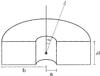 |
Fig. 5 Sketch of the PK model (Pier & Krolik 1992). The inner radius, a, outer radius, b and height, h are marked, and the torus is viewed from angle i, measured as shown. The central nucleus is indicated by an asterisk. The density is assumed to be constant throughout the torus. |
Parameters of the torus model.
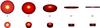 |
Fig. 6 Modelled tori for τr/τz = 10 (top, model w, disky) and τr/τz = 1 (bottom, model c, chunky) for increasing inclinations. Note the appearance of the central engine at 45° (light blue point), and the complete disappearance of the hottest part for 90° (yellow area) due to the cylindrical configuration. This artificially emphasises the difference of the SEDs in the range 85° < i < 90°. |
The main goal of this approach is to find a physically meaningful geometry which can give an adequate description of the entire sample, to estimate torus inclinations and thereby to test the general configuration mentioned in Sect. 1. We have considered a set of representative candidate models, as listed in Table 4.
Some reasonable arguments and previous observations help us to define the average geometry and to select among the models in Table 4. First, the statistical study of the relative frequency of type 1 and 2 AGN by Barthel (1989) implies a torus opening angle θ ~ 45°, which corresponds to a/h ~ 0.3 in the PK models. Second, X-ray observations of nearby AGN (e.g. NGC 1068) set a lower limit on the torus opacity of τ ≥ 1 (Mulchaey et al. 1992). Only the c and w model geometries satisfy both criteria. The main difference between these geometries is illustrated in Fig. 6: they have chunky (c) and disky (w) shapes, respectively.
A more objective approach is to give each model a score based on the goodness of fit averaged over the whole sample. The fit again uses χ2 minimization with two free parameters per fit: the normalization of each model and the inclination i of the torus. This score (rightmost column of Table 4) is the number of “reasonable” fits, i.e. those with an associated probability of >95%. The average score is therefore an indicator of how well the model fits the samples: higher scores correspond to models which performed better at modelling the observed SEDs. Fig. 7 shows the inclination distribution for the four geometries with the best scores for both samples (s3CR and sSHzRG). Models with narrow opening angles (e.g. b and f, and d to a lesser extent) artificially bias the distribution towards low inclinations. We therefore do not use the scores in Table 4 to simply select between all the torus geometries; instead, the scores are used to select only between models c and w, which already meet criteria set by the physical arguments and observations described above. Of these, we select c, which has the higher score (Table 4). The inclinations i from model c with their 5 μm rest frame monochromatic energies of the torus model  are reported in Table 5 and Table 6 for the sSHzRG and s3CR samples, respectively. Their SEDs are presented in Figs. 11 and 12. Section 5 discusses these inclinations in more detail.
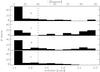 |
Fig. 7 Distribution of inclination angles i for the four best-scoring models. The vertical dashed line indicates i = 45°. |
Figure 8 shows a plot of core dominance R against the inclination i derived from the mid-IR observations. The distribution of the points in the diagram suggests an anti-correlation between i and R, which is confirmed with a generalized Spearman rank test for the sSHzRG sample alone (p = 0.011). Adding the s3CR sample causes the correlation to become extremely significant (p < 0.0001), but note that this is primarily because of the inclusion of the (less obscured) s3CR quasars, which extends the ranges of both R and i.
We would like to add a cautionary note on using the individual inclinations at face value. One source of uncertainty stems from the misalignment of the radio jets with respect to the torus axis This misalignment adds an intrinsic scatter in the R-i relation. A similar scatter is observed in the plane of the sky through polarimetric measurements.
The distribution of inclinations within 0° < i ≲ 45° is inconsistent with the expectations for an isotropically-distributed parent sample: far too many values are clustered around i ≈ 0° or i ≈ 30°. In particular, inclinations close to i ≈ 0 seem suspicious since they would be expected for blazars which are absent from our sample.
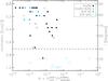 |
Fig. 8 Plot of inclination i against core dominance R. The dashed line at i = 45° corresponds to the division between radio galaxies and quasars derived by Barthel (1989). Filled diamonds represent the type 2 radio galaxies from the sSHzRG (black) and s3CR (blue) samples, respectively. Open symbols represent: sSHzRG broad-line radio galaxies (black diamonds) and s3CR quasars (blue squares). |
5. Discussion
5.1. From extinction to inclination
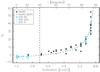 |
Fig. 9 Inclination i obtained from the torus model plotted against extinction AV from the empirical approach. The dashed vertical line is plotted at i = 45°, and the dashed curve corresponds to Eq. (1). |
Both the empirical approach (Sect. 4.3) and the torus model (Sect. 4.4) successfully fit the hot dust emission. We now check the consistency between these two methods by comparing the empirical extinction and the orientation from our best torus model. As shown in Fig. 9, these two parameters are tightly correlated. Their relation is well described by the following function: 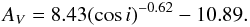 (1)Since the link between extinction and inclination is essentially determined by the geometry of the torus, the small scatter provides support for our choice of a single torus model (c) for the entire sample (sSHzRG and s3CR).
5.2. Isolating the torus emission
5.2.1. Stellar and extended warm dust emission
Here, we investigate the impact of the assumptions made in Sect. 4.1 to isolate the hot dust component from all other contributions in the SED. As we assume that the main stellar contribution is dominated by an evolved population (>500 Myr old), all galaxies of our sample have already formed the bulk of their stellar mass (see S07). The SED of such a population has a characteristic shape for λrest ≳ 1.6 μm, as illustrated by the stellar SEDs plotted in Fig. 11. This shape is relatively independent of age, since the light is dominated by low-mass stars. The assumption of a single high formation redshift therefore has minor consequences for the separation of stellar and hot dust components.
A more important aspect is the SED coverage, which varies systematically with redshift. The number of data points measuring purely stellar emission depends on the sampling beyond the stellar bump (~1.6 μm) and the relative hot dust contribution in the redmost stellar dominated IRAC channel. This may, for instance, cause an overestimate of stellar emission for z < 2 and lead to a higher inclination and extinction estimate. However, we do not observe such a redshift bias in the sSHzRG sample. On the other hand, the s3CR sample, which contains only z < 2 objects, may be more affected by this effect. We indeed find that s3CR type 2 sources mostly have a high derived inclination (70° < i < 90°). Adding near-IR photometry could solve this problem, but this is not available for most of this sample.
Similarly, the reddest end of the SED may be affected by extended warm dust emission. To minimize this problem, we cut at 8 μm as explained in Sect. 4.1. Nevertheless, in some cases, a rising spectrum from λobs = 16 μm to λobs ≥ 24 μm (e.g. MRC 0152−209, MRC 0406−244) suggests that even at λrest = 8 μm, a contribution from such a component cannot be excluded.
Indeed, we note that most of the galaxies for which the fit converged to the highest inclination (i.e. the reddest model) may be affected (MRC 0211−256, MRC 0324−228, 6CE 0905+3955, 3C 356, 3C 368, 7C 1805+6332, 3C 470). This could partially explain the clustering of points at i = 86°. To test the influence of this contamination, we reduced by a factor of three the flux in the redmost filter for these seven sources. The effect is small: the inclination only decreases in three of them, with a maximum change of 7°. To quantify this effect, a tightly sampled SED over the wavelength range 8 μm < λrest ≲ 20 μm would be required. Alternatively, we would have to isolate the torus spatially from more extended emission. This has been attempted for nearby type 2 AGN (van der Wolk et al. 2010) where such an extended component has indeed been identified at λrest = 12 μm. Both types of observation are beyond the reach of current facilities for our samples.
5.2.2. Additional complications for type 1 AGN
In addition to the difficulty of estimating the inclination of an individual type 1 AGN, as described in Sects. 4.3 and 4.4, there are two further complications: at the blue end of the spectrum, transmitted quasar continuum emission can still outshine both the host galaxy and the hot dust emission from the torus. The PK model already includes the power-law emission from the AGN. As explained in Sect. 4.1, we have not included a contribution from the host galaxy in fitting type 1 AGN. As a test, we have included this component in the same way as in the type 2 AGN, i.e. assuming that the bluest IRAC point is 100% stellar emission. In all 11 s3CR quasars, we find that adding this stellar component severely degrades the quality of the fit, but even in this extreme case, the R-i correlation still remains significant at the p = 0.002 level. It is still possible that a smaller stellar component has a smaller contribution on the blue end. Subtracting such a partial stellar population would slightly increase the inclinations found.
On the red end of the torus emission, some sources may also have a contribution from core synchrotron emission (Cleary et al. 2007). This effect is similar to the extended dust component described above, but given the relative small core dominance in our samples (Tables 1 and 3), we do not expect such contributions to have a significant effect.
Despite the above complications, we do find that all quasars have i < 45° (see Fig. 8) as expected from unified models.
5.3. The relative orientations of jets and tori
Our mid-IR SED fitting provides the first estimates of AGN torus inclinations at high redshift. The significant correlation between the radio core dominance and the torus inclination (Fig. 8) implies that the radio jets are indeed generally orthogonal to the equatorial plane of the torus. Orthogonality in projection on the plane of the sky had already been inferred from polarimetric measurements (e.g. Vernet et al. 2001). Our result confirms this geometry in an orthogonal plane containing the line of sight. Together, these observations provide further evidence in favour of the orientation-based unified scheme for AGN.
In the choice of our geometrical model of the torus, we have assumed a half opening angle θ = 45°, as constrained by statistical studies of the relative numbers of type 1 and 2 AGN in a radio-selected sample (Barthel 1989). Other studies have suggested slightly different values of θ (e.g. Willott et al. 2000, find θ = 56°). The torus opening angle may well vary from object to object. This will produce a natural scatter in the R-i relationship. In addition, the transition between direct and obscured view is not expected to be sharp due to the clumpiness of the obscuring material. Two classes of radio galaxies are expected to have inclinations near this transition region. First, radio galaxies with observed broad Hα emission (Humphrey et al. 2008; Nesvadba et al. 2011), are indeed found at 45° < i < 75° (open diamonds in Fig. 8). Second, the two radio galaxies with observed broad absorption lines (MRC 2025−218 and TXS J1908+7220; Humphrey et al. 2008; De Breuck et al. 2001), have i = 46° and i = 59°, respectively, consistent with the expectation to observe them near the grazing line of sight along the torus (e.g. Ogle et al. 1999).
In addition, the torus model adopted to be most representative for the complete sample may not be the optimal choice for a given object. This is particularly true for type 1 AGN, where we cannot constrain the orientation within the range where we have a direct view of the central source, i.e. 0° < i ≲ 45° (see Sects. 4.3, 4.4 and 5.2.2).
Given these caveats, we deliberately do not quote uncertainties on i. In Sect. 5.4 (below), we use only the inclinations for the Type 2 galaxies.
5.4. Constraints on the core Lorentz factor
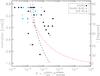 |
Fig. 10 Core dominance R versus inclination i. The black dashed line is the best fit for all type 2 radio galaxies, Γ = 1.3. The red dashed line represents the case Γ = 5. |
Many lines of evidence lead to the conclusion that the jets in radio-loud AGN are relativistic on pc scales, with Lorentz factors of at least 2 and perhaps as high as 50. The highly significant correlation between R and i (Fig. 8) arises naturally if the core radio emission comes from the base of a relativistic jet. If the intrinsic ratio between core and extended emission is constant, then we can use the core dominance for simple assumptions about the jet flow. For anti-parallel, identical jets with velocity βc (Lorentz factor Γ = (1 − β2) − 1/2) and spectral index α at an angle i to the line of sight, the predicted value of R is:
![Mathematical equation: $$ R = R_0 \left[(1-\beta\cos i)^{-(2-\alpha)} + (1+\beta\cos i)^{-(2-\alpha)}\right] $$](/articles/aa/full_html/2012/12/aa20059-12/aa20059-12-eq124.png) where 2R0 is the value of R when the jets are in the plane of the sky (i = 90°).
where 2R0 is the value of R when the jets are in the plane of the sky (i = 90°).
Figure 10 plots R against i for all of the type 2 radio galaxies (sSHzRG and s3CR) with measured R values. For a spectral index α = −0.9 (the median value of both samples), the best-fitting Lorentz factor derived from an unweighted least-squares fit to the relation between log R and i is Γ = 1.3, with R0 = 10-4. As our type 2 samples are restricted to inclinations i > 30°, the Lorentz factor is not well constrained (the dependence of R on i is quite flat). Only very low values of Γ are firmly excluded, and adequate fits can be found for any Γ ≳ 1.3 (for example, see Fig. 10, where the red dashed line represents Γ = 5). The dispersion in log R for the best-fitting Γ is 0.59. A stronger constraint on Γ could be obtained from the R − i relation for a comparable sample of broad-lined objects (or just from the median value of R if inclinations are not available). As noted earlier (Sect. 5.3), we do not believe that our estimates of inclination for the s3CR quasars are reliable enough for this purpose.
One potential source of additional scatter in the relation between core dominance and inclination is any dependence of the intrinsic core/extended ratio on luminosity. Such a dependence was found by Giovannini et al. (1988) for a sample of sources covering a wide range in luminosity. We have checked for this effect over the restricted luminosity range of the present type 2 sample, but find no detectable correlation between core dominance and luminosity (Fig. 2).
The most appropriate comparison study in the literature is a Bayesian analysis of the core dominance distribution for a sample of powerful FR II radio sources including both broad and narrow-line objects at z < 1 (Mullin & Hardcastle 2009). This gave  with a dispersion of 0.62 in log R assuming a single value of Γ and a dispersion in intrinsic core dominance. A value of Γ = 10, would also be fully consistent with the present data. The jet/counter-jet ratio on kpc scales provides an independent estimate of orientation. This can be measured adequately only for nearby, low-luminosity radio galaxies, for which Laing et al. (1999) found Γ = 2.4 and a dispersion of 0.45 in log R.
Various lines of argument suggest that parsec-scale jets have velocity gradients and that the single-velocity model used here is oversimplified. If this is the case, then our analysis is sensitive to the slowest-moving component which makes a significant contribution to the rest-frame emission. Faster material will dominate only at smaller angles to the line of sight.
We conclude that the relation between core dominance and inclination for the present sample of high-redshift radio galaxies is fully consistent with their cores being the bases of relativistic jets, as inferred for radio-loud AGN at lower redshift, but that we can set only a lower bound on the Lorentz factor, Γ ≳ 1.3 without additional data.
6. Summary and conclusions
We have examined the relative inclinations of jets and tori in powerful radio-loud AGN at z > 1. To estimate the orientation of the radio jets, we have introduced a new definition of the radio core dominance R as the ratio between high-frequency, anisotropic core emission and low-frequency, isotropic extended emission, both measured in the rest frame. To estimate the orientation of the dusty torus, we fit optically-thick radiative transfer models to existing and new Spitzer 3.6–24 μm photometry. To isolate the hot dust emission in the torus from non-thermal and host galaxy contributions, we subtract an evolved stellar population in the type 2 sources, and restrict to the 2 μm < λrest < 8 μm region.
Using this method, we derive radio core dominance and torus inclination values for 42 type 2 and 11 type 1 AGN. This mid-IR determination of the inclination allows us to draw the following conclusions:
-
1.
The significant correlation between R and i implies that radio jets are indeed approximately orthogonal to the equatorial plane of the torus as predicted by the orientation-based AGN unified scheme. A similar result in the plane of the sky has been reported using polarimetric measurements, but our results provide additional evidence in the complementary direction, i.e. along the line of sight.
-
2.
The R–i correlation is consistent with the radio cores being the bases of relativistic jets with Lorentz factors Γ ≳ 1.3.
-
3.
Assuming our torus geometry is representative, we can estimate inclinations for larger samples of type 2 AGN using the relation (Eq. (1)) between inclination and the obscuration AV as derived from a simple reddening of a mean type 1 template.
The present study characterises the anisotropic component of the dust IR SED in type 2 AGN. The remaining more isotropic dust emission, dominating at longer wavelenghts, is powered by a combination of AGN and starbursts. Our new Projet HeRGÉ aims to disentangle these two contributions by adding Herschel 70–500 μm photometry (Seymour et al. 2012) to our sample of 71 radio galaxies at 1 < z < 5.2.
Online material
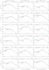 |
Fig. 11 Mid-IR SEDs for the sSHzRG sample. Black points: photometric data. Green points: measurements used to normalise the contribution from an old stellar population. Red points: results after subtraction of the stellar contribution. Dashed green line: model stellar emission. Dashed red line: best-fitting torus model. Full black line: sum of stellar and torus models. |
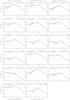 |
Fig. 11 continued. |
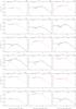 |
Fig. 12 continued. |
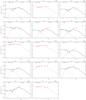 |
Fig. 12 continued. |
Radio data for the SHzRG sample from the literature and core dominance calculated.
3CR sample, Spitzer observations.
Acknowledgments
We thank the referee for the careful reading of the manuscript and their constructive comments. The authors thank K. Blundell for useful comments and her participation in the improvement of this paper and C. Leipski for reanalysing some of the 3CR photometry. Nick Seymour is the recipient of an Australian Research Council Future Fellowship. This work is based on observations made with the Spitzer Space Telescope, which is operated by the Jet Propulsion Laboratory, California Institute of Technology under contract with NASA.
References
- Antonucci, R. 1993, ARA&A, 31, 473 [Google Scholar]
- Antonucci, R. R. J., & Miller, J. S. 1985, ApJ, 297, 621 [NASA ADS] [CrossRef] [Google Scholar]
- Athreya, R. M., Kapahi, V. K., McCarthy, P. J., & van Breugel, W. 1997, MNRAS, 289, 525 [NASA ADS] [CrossRef] [Google Scholar]
- Barthel, P. D. 1989, ApJ, 336, 606 [Google Scholar]
- Best, P. N., Longair, M. S., & Roettgering, J. H. A. 1997, MNRAS, 292, 758 [NASA ADS] [CrossRef] [Google Scholar]
- Best, P. N., Kauffmann, G., Heckman, T. M., et al. 2005, MNRAS, 362, 25 [NASA ADS] [CrossRef] [Google Scholar]
- Blandford, R. D., & Payne, D. G. 1982, MNRAS, 199, 883 [NASA ADS] [CrossRef] [Google Scholar]
- Blundell, K. M., Rawlings, S., Eales, S. A., Taylor, G. B., & Bradley, A. D. 1998, MNRAS, 295, 265 [NASA ADS] [CrossRef] [Google Scholar]
- Blundell, K. M., Rawlings, S., & Willott, C. J. 1999, AJ, 117, 677 [Google Scholar]
- Broderick, J. W., De Breuck, C., Hunstead, R. W., & Seymour, N. 2007, MNRAS, 375, 1059 [NASA ADS] [CrossRef] [Google Scholar]
- Cai, Z., Nan, R., Schilizzi, R. T., et al. 2002, A&A, 381, 401 [NASA ADS] [CrossRef] [EDP Sciences] [Google Scholar]
- Carilli, C. L., Owen, F. N., & Harris, D. E. 1994, AJ, 107, 480 [NASA ADS] [CrossRef] [Google Scholar]
- Carilli, C. L., Roettgering, H. J. A., van Ojik, R., Miley, G. K., & van Breugel, W. J. M. 1997, ApJS, 109, 1 [NASA ADS] [CrossRef] [Google Scholar]
- Chambers, K. C., Miley, G. K., van Breugel, W. J. M., et al. 1996, ApJS, 106, 247 [NASA ADS] [CrossRef] [Google Scholar]
- Cimatti, A., di Serego-Alighieri, S., Fosbury, R. A. E., Salvati, M., & Taylor, D. 1993, MNRAS, 264, 421 [NASA ADS] [CrossRef] [Google Scholar]
- Cleary, K., Lawrence, C. R., Marshall, J. A., Hao, L., & Meier, D. 2007, ApJ, 660, 117 [NASA ADS] [CrossRef] [Google Scholar]
- Corbin, M. R., Charlot, S., De Young, D. S., Owen, F., & Dunlop, J. S. 1998, ApJ, 496, 803 [NASA ADS] [CrossRef] [Google Scholar]
- De Breuck, C., van Breugel, W., Röttgering, H. J. A., & Miley, G. 2000, A&AS, 143, 303 [NASA ADS] [CrossRef] [EDP Sciences] [Google Scholar]
- De Breuck, C., van Breugel, W., Röttgering, H., et al. 2001, AJ, 121, 1241 [NASA ADS] [CrossRef] [Google Scholar]
- De Breuck, C., Seymour, N., Stern, D., et al. 2010, ApJ, 725, 36 [NASA ADS] [CrossRef] [Google Scholar]
- di Serego Alighieri, S., Fosbury, R. A. E., Tadhunter, C. N., & Quinn, P. J. 1989, Nature, 341, 307 [NASA ADS] [CrossRef] [Google Scholar]
- di Serego Alighieri, S., Cimatti, A., & Fosbury, R. A. E. 1993, ApJ, 404, 584 [NASA ADS] [CrossRef] [Google Scholar]
- Dullemond, C. P., & van Bemmel, I. M. 2005, A&A, 436, 47 [NASA ADS] [CrossRef] [EDP Sciences] [Google Scholar]
- Fazio, G. G., Hora, J. L., Allen, L. E., et al. 2004, ApJS, 154, 10 [NASA ADS] [CrossRef] [Google Scholar]
- Ferrarese, L., & Merritt, D. 2000, ApJ, 539, L9 [NASA ADS] [CrossRef] [Google Scholar]
- Fioc, M., & Rocca-Volmerange, B. 1997, A&A, 326, 950 [NASA ADS] [Google Scholar]
- Fitzpatrick, E. L. 1999, PASP, 111, 63 [NASA ADS] [CrossRef] [Google Scholar]
- Fomalont, E. B., Kellermann, K. I., Partridge, R. B., Windhorst, R. A., & Richards, E. A. 2002, AJ, 123, 2402 [NASA ADS] [CrossRef] [Google Scholar]
- Fritz, J., Franceschini, A., & Hatziminaoglou, E. 2006, MNRAS, 366, 767 [Google Scholar]
- Giovannini, G., Feretti, L., Gregorini, L., & Parma, P. 1988, A&A, 199, 73 [NASA ADS] [Google Scholar]
- Granato, G. L., & Danese, L. 1994, MNRAS, 268, 235 [NASA ADS] [CrossRef] [Google Scholar]
- Haas, M., Klaas, U., Müller, S. A. H., et al. 2003, A&A, 402, 87 [NASA ADS] [CrossRef] [EDP Sciences] [Google Scholar]
- Haas, M., Willner, S. P., Heymann, F., et al. 2008, ApJ, 688, 122 [NASA ADS] [CrossRef] [Google Scholar]
- Hines, D. C. 1994, Ph.D. Thesis, Texas University [Google Scholar]
- Hoekstra, H., Barthel, P. D., & Hes, R. 1997, A&A, 319, 757 [NASA ADS] [Google Scholar]
- Hönig, S. F., Beckert, T., Ohnaka, K., & Weigelt, G. 2006, A&A, 452, 459 [NASA ADS] [CrossRef] [EDP Sciences] [Google Scholar]
- Houck, J. R., Roellig, T. L., van Cleve, J., et al. 2004, ApJS, 154, 18 [NASA ADS] [CrossRef] [Google Scholar]
- Humphrey, A., Villar-Martín, M., Vernet, J., et al. 2008, MNRAS, 383, 11 [NASA ADS] [CrossRef] [Google Scholar]
- Ibar, E., & Lira, P. 2007, A&A, 466, 531 [NASA ADS] [CrossRef] [EDP Sciences] [Google Scholar]
- Kapahi, V. K. & Saikia, D. J. 1982, J. Astrophys. Astron., 3, 465 [Google Scholar]
- Kapahi, V. K., Athreya, R. M., van Breugel, W., McCarthy, P. J., & Subrahmanya, C. R. 1998, ApJS, 118, 275 [NASA ADS] [CrossRef] [Google Scholar]
- Kishimoto, M., Hönig, S. F., Antonucci, R., et al. 2011, A&A, 536, A78 [NASA ADS] [CrossRef] [EDP Sciences] [Google Scholar]
- Krolik, J. H., & Begelman, M. C. 1988, ApJ, 329, 702 [NASA ADS] [CrossRef] [Google Scholar]
- Laing, R. A., Parma, P., de Ruiter, H. R., & Fanti, R. 1999, MNRAS, 306, 513 [NASA ADS] [CrossRef] [Google Scholar]
- Law-Green, J. D. B., Eales, S. A., Leahy, J. P., Rawlings, S., & Lacy, M. 1995a, MNRAS, 277, 995 [NASA ADS] [Google Scholar]
- Law-Green, J. D. B., Leahy, J. P., Alexander, P., et al. 1995b, MNRAS, 274, 939 [NASA ADS] [Google Scholar]
- Leipski, C., Haas, M., Willner, S. P., et al. 2010, ApJ, 717, 766 [NASA ADS] [CrossRef] [Google Scholar]
- Matthews, T. A., Morgan, W. W., & Schmidt, M. 1964, ApJ, 140, 35 [NASA ADS] [CrossRef] [Google Scholar]
- McCarthy, P. J., van Breugel, W., Spinrad, H., & Djorgovski, S. 1987, ApJ, 321, L29 [NASA ADS] [CrossRef] [Google Scholar]
- McCarthy, P. J., Spinrad, H., Dickinson, M., et al. 1990, ApJ, 365, 487 [NASA ADS] [CrossRef] [Google Scholar]
- McCarthy, P. J., van Breugel, W., & Kapahi, V. K. 1991, ApJ, 371, 478 [NASA ADS] [CrossRef] [Google Scholar]
- McLure, R. J., Jarvis, M. J., Targett, T. A., Dunlop, J. S., & Best, P. N. 2006, MNRAS, 368, 1395 [NASA ADS] [CrossRef] [Google Scholar]
- Mulchaey, J. S., Myshotzky, R. F., & Weaver, K. A. 1992, ApJ, 390, L69 [NASA ADS] [CrossRef] [Google Scholar]
- Mullin, L. M., & Hardcastle, M. J. 2009, MNRAS, 398, 1989 [NASA ADS] [CrossRef] [Google Scholar]
- Nenkova, M., Ivezić, Ž., & Elitzur, M. 2002, ApJ, 570, L9 [NASA ADS] [CrossRef] [Google Scholar]
- Nenkova, M., Sirocky, M. M., Ivezić, Ž., & Elitzur, M. 2008, ApJ, 685, 147 [NASA ADS] [CrossRef] [Google Scholar]
- Nesvadba, N. P. H., Lehnert, M. D., De Breuck, C., Gilbert, A. M., & van Breugel, W. 2008, A&A, 491, 407 [NASA ADS] [CrossRef] [EDP Sciences] [Google Scholar]
- Nesvadba, N. P. H., De Breuck, C., Lehnert, M. D., et al. 2011, A&A, 525, A43 [NASA ADS] [CrossRef] [EDP Sciences] [Google Scholar]
- Ogle, P. M., Cohen, M. H., Miller, J. S., et al. 1999, ApJS, 125, 1 [NASA ADS] [CrossRef] [Google Scholar]
- Pentericci, L., Van Reeven, W., Carilli, C. L., Röttgering, H. J. A., & Miley, G. K. 2000, A&AS, 145, 121 [NASA ADS] [CrossRef] [EDP Sciences] [Google Scholar]
- Pentericci, L., McCarthy, P. J., Röttgering, H. J. A., et al. 2001, ApJS, 135, 63 [NASA ADS] [CrossRef] [Google Scholar]
- Pérez-Torres, M.-A., & De Breuck, C. 2005, MNRAS, 363, L41 [NASA ADS] [Google Scholar]
- Pier, E. A., & Krolik, J. H. 1992, ApJ, 401, 99 [NASA ADS] [CrossRef] [Google Scholar]
- Pier, E. A., & Krolik, J. H. 1993, ApJ, 418, 673 [NASA ADS] [CrossRef] [Google Scholar]
- Ramos Almeida, C., Levenson, N. A., Rodríguez Espinosa, J. M., et al. 2009, ApJ, 702, 1127 [NASA ADS] [CrossRef] [Google Scholar]
- Rees, M. J. 1984, ARA&A, 22, 471 [NASA ADS] [CrossRef] [Google Scholar]
- Reuland, M., van Breugel, W., Röttgering, H., et al. 2003, ApJ, 592, 755 [NASA ADS] [CrossRef] [Google Scholar]
- Richards, G. T., Lacy, M., Storrie-Lombardi, L. J., et al. 2006, ApJS, 166, 470 [NASA ADS] [CrossRef] [Google Scholar]
- Rieke, G. H., Young, E. T., Engelbracht, C. W., et al. 2004, ApJS, 154, 25 [NASA ADS] [CrossRef] [Google Scholar]
- Rigby, E. E., Snellen, I. A. G., & Best, P. N. 2007, MNRAS, 380, 1449 [NASA ADS] [CrossRef] [Google Scholar]
- Rowan-Robinson, M. 1995, MNRAS, 272, 737 [NASA ADS] [Google Scholar]
- Sanders, D. B., Soifer, B. T., Elias, J. H., et al. 1988, ApJ, 325, 74 [NASA ADS] [CrossRef] [Google Scholar]
- Schartmann, M., Meisenheimer, K., Camenzind, M., Wolf, S., & Henning, T. 2005, A&A, 437, 861 [NASA ADS] [CrossRef] [EDP Sciences] [Google Scholar]
- Scheuer, P. A. G., & Readhead, A. C. S. 1979, Nature, 277, 182 [NASA ADS] [CrossRef] [Google Scholar]
- Seymour, N., Stern, D., De Breuck, C., et al. 2007, ApJS, 171, 353 [NASA ADS] [CrossRef] [Google Scholar]
- Seymour, N., Ogle, P., De Breuck, C., et al. 2008, ApJ, 681, L1 [NASA ADS] [CrossRef] [Google Scholar]
- Seymour, N., Altieri, B., De Breuck, C., et al. 2012, ApJ, 755, 146 [NASA ADS] [CrossRef] [Google Scholar]
- Smail, I., Swinbank, A. M., Ivison, R. J., & Ibar, E. 2011, MNRAS, 414, L95 [NASA ADS] [CrossRef] [Google Scholar]
- Spinrad, H., Marr, J., Aguilar, L., & Djorgovski, S. 1985, PASP, 97, 932 [NASA ADS] [CrossRef] [Google Scholar]
- Stalevski, M., Fritz, J., Baes, M., Nakos, T., & Popović, L. Č. 2012, MNRAS, 420, 2756 [NASA ADS] [CrossRef] [Google Scholar]
- Tran, H. D., Miller, J. S., & Kay, L. E. 1992, ApJ, 397, 452 [NASA ADS] [CrossRef] [Google Scholar]
- van Bemmel, I. M., & Dullemond, C. P. 2003, A&A, 404, 1 [NASA ADS] [CrossRef] [EDP Sciences] [Google Scholar]
- van Breugel, W. J. M., Stanford, S. A., Spinrad, H., Stern, D., & Graham, J. R. 1998, ApJ, 502, 614 [NASA ADS] [CrossRef] [Google Scholar]
- van der Wolk, G., Barthel, P. D., Peletier, R. F., & Pel, J. W. 2010, A&A, 511, A64 [NASA ADS] [CrossRef] [EDP Sciences] [Google Scholar]
- van Ojik, R., Roettgering, H. J. A., Carilli, C. L., et al. 1996, A&A, 313, 25 [NASA ADS] [Google Scholar]
- Vernet, J., Fosbury, R. A. E., Villar-Martín, M., et al. 2001, A&A, 366, 7 [NASA ADS] [CrossRef] [EDP Sciences] [Google Scholar]
- Villar-Martín, M., Vernet, J., di Serego Alighieri, S., et al. 2003, MNRAS, 346, 273 [NASA ADS] [CrossRef] [Google Scholar]
- Werner, M. W., Roellig, T. L., Low, F. J., et al. 2004, ApJS, 154, 1 [Google Scholar]
- White, R. L., Becker, R. H., Helfand, D. J., & Gregg, M. D. 1997, ApJ, 475, 479 [NASA ADS] [CrossRef] [Google Scholar]
- Willott, C. J., Rawlings, S., Blundell, K. M., & Lacy, M. 2000, MNRAS, 316, 449 [NASA ADS] [CrossRef] [Google Scholar]
Appendix A: Notes on individual sources
B3 J2330+3927 This galaxy has the highest core dominance in the SHzRG sample (R = 0.004). The radio emission is complex (Pérez-Torres & De Breuck 2005).
6C 0140+326 This source (the second highest redshift source in the SHzRG sample) has been removed from this study, as a foreground object contaminates the galaxy image in the IRAC bands.
4C 60.07, 3C 356, MRC 2048−272, 7C 1756+5620. These four objects have double components in the IRAC maps, but only one of each pair coincides with a radio core.
MRC 2025−218, MRC 0156−252, MRC 1017−220, TXS 1113−178, MRC 1138−262, MRC 1558−003, MRC 0251−273 These galaxies show broad permitted lines (Nesvadba et al. 2011; Humphrey et al. 2008).
6C 0032+412 This galaxy exhibits a very hot dust component in its mid-IR SED (De Breuck et al. 2010).
TNJ2007−1316 The previously quoted flux density at 5.6 μm has been replaced with a 3σ upper limit of F5.6 μm < 146.0 μJy.
All Tables
Radio data for the SHzRG sample from the literature and core dominance calculated.
All Figures
|
Fig. 1 Core dominance R versus redshift. Note the lower redshifts for the s3CR sample (blue diamonds and open squares). The open black diamonds correspond to radio galaxies with observed broad lines, see Sect. 5.3. |
| In the text | |
|
Fig. 2 Core dominance R versus |
| In the text | |
|
Fig. 3 Template SEDs for the empirical approach. The black curve is the mean quasar spectrum from Richards et al. (2006). The bluer/redder curves correspond to a increasing extinction (from –12 to 90 Av in steps of 6), using the Fitzpatrick (1999) extinction law. |
| In the text | |
|
Fig. 4 Extinction AV versus core dominance R. Note the absence of points in the top right part of the plot. This figure is consistent with Fig. 12 of Cleary et al. (2007). |
| In the text | |
|
Fig. 5 Sketch of the PK model (Pier & Krolik 1992). The inner radius, a, outer radius, b and height, h are marked, and the torus is viewed from angle i, measured as shown. The central nucleus is indicated by an asterisk. The density is assumed to be constant throughout the torus. |
| In the text | |
|
Fig. 6 Modelled tori for τr/τz = 10 (top, model w, disky) and τr/τz = 1 (bottom, model c, chunky) for increasing inclinations. Note the appearance of the central engine at 45° (light blue point), and the complete disappearance of the hottest part for 90° (yellow area) due to the cylindrical configuration. This artificially emphasises the difference of the SEDs in the range 85° < i < 90°. |
| In the text | |
|
Fig. 7 Distribution of inclination angles i for the four best-scoring models. The vertical dashed line indicates i = 45°. |
| In the text | |
|
Fig. 8 Plot of inclination i against core dominance R. The dashed line at i = 45° corresponds to the division between radio galaxies and quasars derived by Barthel (1989). Filled diamonds represent the type 2 radio galaxies from the sSHzRG (black) and s3CR (blue) samples, respectively. Open symbols represent: sSHzRG broad-line radio galaxies (black diamonds) and s3CR quasars (blue squares). |
| In the text | |
|
Fig. 9 Inclination i obtained from the torus model plotted against extinction AV from the empirical approach. The dashed vertical line is plotted at i = 45°, and the dashed curve corresponds to Eq. (1). |
| In the text | |
|
Fig. 10 Core dominance R versus inclination i. The black dashed line is the best fit for all type 2 radio galaxies, Γ = 1.3. The red dashed line represents the case Γ = 5. |
| In the text | |
|
Fig. 11 Mid-IR SEDs for the sSHzRG sample. Black points: photometric data. Green points: measurements used to normalise the contribution from an old stellar population. Red points: results after subtraction of the stellar contribution. Dashed green line: model stellar emission. Dashed red line: best-fitting torus model. Full black line: sum of stellar and torus models. |
| In the text | |
|
Fig. 11 continued. |
| In the text | |
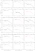 |
Fig. 12 Mid-IR SEDs for the s3CR sample. The symbols are the same than in Fig. 11. |
| In the text | |
|
Fig. 12 continued. |
| In the text | |
|
Fig. 12 continued. |
| In the text | |
Current usage metrics show cumulative count of Article Views (full-text article views including HTML views, PDF and ePub downloads, according to the available data) and Abstracts Views on Vision4Press platform.
Data correspond to usage on the plateform after 2015. The current usage metrics is available 48-96 hours after online publication and is updated daily on week days.
Initial download of the metrics may take a while.