| Issue |
A&A
Volume 547, November 2012
|
|
|---|---|---|
| Article Number | A90 | |
| Number of page(s) | 24 | |
| Section | Stellar atmospheres | |
| DOI | https://doi.org/10.1051/0004-6361/201219778 | |
| Published online | 06 November 2012 | |
Magnetic fields of HgMn stars⋆,⋆⋆
1
Leibniz-Institut für Astrophysik Potsdam (AIP),
An der Sternwarte 16,
14482
Potsdam, Germany
e-mail: This email address is being protected from spambots. You need JavaScript enabled to view it.
2
Instituto de Ciencias Astronomicas, de la Tierra, y del Espacio (ICATE),
5400
San Juan,
Argentina
3
Niels Bohr Institute, University of Copenhagen,
Juliane Maries Vej 30,
2100
København,
Denmark
4
Centre for Star and Planet Formation, Natural History Museum of
Denmark, University of Copenhagen, Øster Voldgade 5-7, 1350
Copenhagen,
Denmark
5
European Southern Observatory, Karl-Schwarzschild-Str. 2, 85748
Garching bei München,
Germany
6
Institute of Astronomy, Russian Academy of Sciences,
Pyatnitskaya 48, 119017
Moscow,
Russia
7
Instituto Nazionale di Astrofisica, Osservatorio Astronomico di
Trieste, via Tiepolo
11, 34143
Trieste,
Italy
8
Instituut voor Sterrenkunde, K.U. Leuven,
Celestijnenlaan 200D,
3001
Leuven,
Belgium
9
Institut d’Astrophysique et de Géophysique Université de Liège,
Allée du 6 Août 17,
4000
Liège,
Belgium
Received:
8
June
2012
Accepted:
30
July
2012
Abstract
Context. The frequent presence of weak magnetic fields on the surface of spotted late-B stars with HgMn peculiarity in binary systems has been controversial during the two last decades. Recent studies of magnetic fields in these stars using the least-squares deconvolution (LSD) technique have failed to detect magnetic fields, indicating an upper limit on the longitudinal field between 8 and 15 G. In these LSD studies, assumptions were made that all spectral lines are identical in shape and can be described by a scaled mean profile.
Aims. We re-analyse the available spectropolarimetric material by applying the moment technique on spectral lines of inhomogeneously distributed elements separately. Furthermore, we present new determinations of the mean longitudinal magnetic field for the HgMn star HD 65949 and the hotter analog of HgMn stars, the PGa star HD 19400, using FORS 2 installed at the VLT. We also give new measurements of the eclipsing system AR Aur with a primary star of HgMn peculiarity, which were obtained with the SOFIN spectropolarimeter installed at the Nordic Optical Telescope.
Methods. We downloaded from the European Southern Observatory (ESO) archive the publically available HARPS spectra for eight HgMn stars and one normal and one superficially normal B-type star obtained in 2010. Out of this sample, three HgMn stars belong to spectroscopic double-lined systems. The application of the moment technique to the HARPS and SOFIN spectra allowed us to study the presence of the longitudinal magnetic field, the crossover effect, and quadratic magnetic fields. Results for the HgMn star HD 65949 and the PGa star HD 19400 are based on a linear regression analysis of low-resolution spectra obtained with FORS 2 in spectropolarimetric mode.
Results. Our measurements of the magnetic field with the moment technique using spectral lines of several elements separately reveal the presence of a weak longitudinal magnetic field, a quadratic magnetic field, and the crossover effect on the surface of several HgMn stars as well as normal and superficially normal B-type stars. Furthermore, our analysis suggests the existence of intriguing correlations between the strength of the magnetic field, abundance anomalies, and binary properties. The results are discussed in the context of possible mechanisms responsible for the development of the element patches and complex magnetic fields on the surface of late B-type stars.
Key words: stars: chemically peculiar / stars: atmospheres / binaries: spectroscopic / stars: abundances / stars: early-type / stars: magnetic field
Based on observations obtained at the European Southern Observatory (ESO programmes 076.D-0169(A), 076.D-0172(A), 084.D-0338(A), 085.D-0296(A), 085.D-0296(B), 087.D-0049(A), 088.D-0284(A)), SOFIN observations at the 2.56 m Nordic Optical Telescope on La Palma, and observations obtained with the CORALIE Echelle Spectrograph on the 1.2 m Euler Swiss telescope on La Silla, Chile.
Tables 2–7, 9, 10 are only available in electronic form at http://www.aanda.org
F.R.S.-FNRS Postdoctoral Researcher, Belgium.
© ESO, 2012
1. Introduction
The origin of abundance anomalies observed in late B-type stars with HgMn peculiarity is still poorly understood. Over the last few years, we have performed extensive spectroscopic studies of both single late B-type stars and of spectroscopic binaries (SB) with late B-type primaries (spectral types B7–B9) with the goal of understanding why the vast majority of these stars exhibit in their atmospheres certain chemical abundance anomalies, i.e. large excesses of P, Mn, Ga, Br, Sr, Y, Zr, Rh, Pd, Xe, Pr, Yb, W, Re, Os, Pt, Au, and Hg, and underabundances of He, Al, Zn, Ni, and Co (e.g. Castelli & Hubrig 2004a). Strong isotopic anomalies were detected for the chemical elements Ca, Pt, and Hg, with patterns changing from one star to the next (Hubrig et al. 1999a; Castelli & Hubrig 2004b; Cowley et al. 2010). Observationally, these stars are characterised by low rotational velocities (⟨ v sini ⟩ ≤ 29 km s-1, Abt et al. 1972). The number of these chemically peculiar stars, usually called HgMn stars, decreases with increasing rotational velocity (Wolff & Wolff 1974).
More than two thirds of the HgMn stars are known to belong to spectroscopic binaries (Hubrig & Mathys 1995), with a preference of orbital periods ranging from 3 to 20 days. It is striking that the inspection of SB systems with a late B-type primary in the 9th Catalogue of Spectroscopic Binary Orbits (Pourbaix et al. 2009) indicates a strong correlation between the HgMn peculiarity and membership in a binary system among bright, well-studied SB systems with late B-type, slowly rotating (v sini < 70 km s-1) primaries with an apparent magnitude of up to V ≈ 7 and orbital periods between 3 and 20 d. With the exception of HR 7241, all 21 systems have a primary with a HgMn peculiarity. Based on this fact, it is very likely that the majority of slowly rotating late B-type stars formed in binary systems with certain orbital parameters become HgMn stars. Consequently, careful studies of these peculiar stars are important for the general understanding of B-type star formation in binary systems. According to Abt & Snowden (1973), close-binary formation is inhibited when strong magnetic fields are present. They also suggest that close binaries dissipate the magnetic field.
The aspect of inhomogeneous distribution of some chemical elements over the surface of HgMn stars was first discussed by Hubrig & Mathys (1995). From a survey of HgMn stars in close SBs, it was suggested that some chemical elements might be inhomogeneously distributed on the surface, with, in particular, preferential concentration of Hg along the equator. The first definitively identified spectrum variability was reported for the binary HgMn star α And by Wahlgren et al. (2001) and Adelman et al. (2002), who showed that the spectral variations of the Hg ii line at λ3984 discovered in high-dispersion spectra are not due to the orbital motion of the companion, but produced by the combination of the 2.8 d period of rotation of the primary and a non-uniform surface distribution of mercury, which is concentrated in the equatorial region. Their results are in good correspondence with those of Hubrig & Mathys (1995). The variability of the Hg ii line at λ3984 was interpreted with a Doppler imaging code, revealing high-contrast mercury spots located along the rotational equator. Using a Doppler imaging reconstruction of spectroscopic time series obtained over seven consecutive years, Kochukhov et al. (2007) suggested the presence of a secular evolution of the mercury distribution. On the other hand, the work of other authors has proved that not only mercury abundance appears distributed in patches over the stellar surface. Almost all other elements, most typical Ti, Cr, Fe, Mn, Sr, Y, and Pt, are concentrated in spots of diverse size, and different elements exhibit different abundance distributions across the stellar surface (e.g. Hubrig et al. 2006a; Briquet et al. 2010; Makaganiuk et al. 2011a). Moreover, an evolution of the element abundance spots at different time scales was discovered in two additional HgMn stars. Briquet et al. (2010) reported the presence of dynamical spot evolution over a couple of weeks for the SB1 system HD 11753, while Hubrig et al. (2010) detected a secular element evolution in the double-lined eclipsing binary AR Aur. Importantly, recent results (e.g. Nuñez et al. 2011; Hubrig et al. 2011) show that line-profile variability of various elements caused by a non-uniform abundance distribution is a general characteristic of HgMn stars, rather than an exception.
Typically, inhomogeneous chemical abundance distributions are observed only on the surface of magnetic chemically peculiar stars with large-scale organised magnetic fields (Ap and Bp stars). In these stars, the abundance distribution of certain elements is non-uniform and non-symmetric with respect to the rotation axis. Numerous studies of Ap and Bp stars have revealed a kind of symmetry between the topology of the magnetic field and the element distribution. Thus, the structure of the magnetic field can be studied by measurements of the magnetic field, using spectral lines of each element separately. Although strong large-scale magnetic fields have not generally been found in HgMn stars, it has never been ruled out that these stars might have tangled magnetic fields of the order of a few thousand Gauss with only very weak net longitudinal components. Bychkov et al. (2009) compiled all published longitudinal magnetic field measurements of different groups of chemically peculiar stars and concluded that the group of HgMn stars possesses the second weakest fields after the group of Am stars.
In the last few years, a number of attempts to detect mean longitudinal magnetic fields in HgMn stars have been made by several authors using the line addition technique, the least-squares deconvolution (LSD), most recently by Makaganiuk et al. (e.g. 2011a,b,c). A high level of precision, from a few to tens of Gauss, is achieved through application of the LSD technique (Donati et al. 1997), which combines hundreds of spectral lines of various elements. This technique assumes that all spectral lines are identical in shape and can be described by a scaled mean profile. However, the lines of different elements with different abundance distributions across the stellar surface sample the magnetic field in different manners. Combining them as is done with the LSD technique may lead to the dilution of the magnetic signal or even to its (partial) cancellation, if enhancements of different elements occur in regions of opposite magnetic polarities. Using this technique, Makaganiuk et al. (2011b) analysed HARPS spectra for a sample of HgMn and normal B-type stars and reported no detection at a 3σ level in any of the studied targets.
Strangely enough, although the authors were aware of the inhomogeneous distribution of the elements on the surface of HgMn stars, no analysis has been done on the lines of individual elements separately. Only in the most recent Makaganiuk et al. (2012) study did the authors decide to constrain the longitudinal magnetic field of HD 11753 by computing mean profiles for Y, Ti, and Cr, which show different spot distributions on the stellar surface. Their results indicate that the upper limit for the strength of the magnetic fields can reach about 20–30 G, with a typical error bar from 8 G to 15 G.
To test if the use of the LSD technique may indeed account for the non-detection of magnetic fields in HgMn stars, we decided to re-analyse the HARPS spectropolarimetric material that recently became publically available in the ESO archive. In this work, we use a completely different approach for the measurements of magnetic fields, namely, the moment technique developed by Mathys (e.g. 1991, 1995a,b). This technique allows us not only to determine the mean longitudinal magnetic field, but also to prove the presence of the crossover effect and quadratic magnetic fields. This information cannot be obtained from the LSD technique, as it assumes that all spectral lines are identical in shape and can be described by a scaled mean profile. Furthermore, we present five new spectropolarimetric observations of the eclipsing system AR Aur with a primary star of HgMn peculiarity, obtained with the echelle spectrograph SOFIN at the Nordic Optical Telescope at the end of 2010. The variability and spot distribution of this star has been intensively studied by our group in the few last years (Hubrig et al. 2006a, 2011). In addition, a new set of polarimetric spectra was obtained for the HgMn star HD 65949 and the hotter analog of HgMn stars, the PGa star HD 19400, using FORS 2 installed at the VLT. All targets discussed in this work are presented in Table 1 together with their visual magnitudes and spectral types.
In Sect. 2, we describe the observations, data reduction, and methods of our magnetic field measurements. The stellar characteristics and the magnetic field measurements for the individual targets are reviewed in Sect. 3. Finally, in Sect. 4, we discuss our results in the context of possible mechanisms at play, which can be considered responsible for the development of the inhomogeneous abundance distribution and the presence of weak magnetic fields.
2. Observations and magnetic field measurements
2.1. HARPS observations
The majority of the spectra analyzed in this work were obtained with the HARPSpol polarimeter (Snik et al. 2011) feeding the HARPS spectrometer (Mayor et al. 2003) at the ESO 3.6 m telescope on La Silla. We downloaded from the ESO archive the publically available multi-epoch and single-epoch spectra for eight HgMn stars, one normal B-type star, and one superficially normal B-type star obtained with HARPSpol in 2010. Out of this sample, three HgMn stars belong to spectroscopic double-lined systems. The study of magnetic fields in one normal star and one superficially normal B-type star is of special interest because they were reported as weakly magnetic in previous polarimetric studies. All spectra have a resolving power of R = 115 000 and a signal-to-noise ratio (S/N) between 80 for HD 209 459 and 589 for 41 Eri. The information on the individual observations, including the MJD dates and the S/N values, is given in Table 2. To distinguish between SB1 and SB2 systems, we will call the SB1 systems with their HD number and use the other identifiers given in the second column of Table 1 for the SB2 systems.
The HARPS archive spectra cover the wavelength range 3780–6913 Å, with a small gap around 5300 Å. Each observation of the star is usually split into four to eight sub-exposures, obtained with four different orientations of the quarter-wave retarder plate relative to the beam splitter of the circular polarimeter. The reduction was performed using the HARPS data reduction software available at the ESO headquarters in Germany. The Stokes I and V parameters were derived following the ratio method described by Donati et al. (1997), ensuring in particular that all spurious signatures are removed at first order. Null polarisation spectra (labeled with n in Table 3) were calculated by combining the sub-exposures in such a way that the polarisation cancels out, allowing us to verify that no spurious signals are present in the data. Other details of the typical acquisition and calibration of the HARPSpol observations can be found in papers by Makaganiuk et al. (e.g. 2011a,b).
The diagnostic potential of high-resolution circularly polarised spectra using the moment technique has been discussed at length in numerous papers by Mathys (e.g. 1993, 1995a,b). Wavelength shifts between right- and left-hand side circularly polarised spectra are interpreted in terms of a longitudinal magnetic field ⟨Bz⟩. The major problem in the analysis of high-resolution spectra is the proper line identification of blend-free spectral lines. The quality of the selection varies strongly from star to star, depending on the binarity, the line broadening, and the richness of the spectrum. In addition, due to the inhomogeneous element distribution on the stellar surface, the degree of blending changes with the stellar rotation phase. All the lines we tried to employ in the diagnosis of the magnetic fields on the surface of our target stars are presented in Table 4, together with their Landé factors. We note that the actual list of lines measured in each star on each spectrum can differ from one observation to the next due to the different quality of the spectra and variable blending over the rotation cycle. For the lines of iron-peak elements, the Landé factors were taken from Kurucz’s list of atomic data (Kurucz 1989), while the Landé factors for the Y lines were retrieved from the Vienna Atomic Line Database (VALD; e.g. Kupka et al. 1999).
List of the studied targets.
The measurements of the mean longitudinal magnetic field in our targets using line lists of different elements separately are presented in Table 3. Since the element abundances are different in different stars, only the lines of ions with a larger number of measurable lines were used for the analysis. A study of elements with a small number of lines sets considerable limitations on the amount of information on the presence of a magnetic field. The most populated samples of lines belong to Ti and Fe, followed by Y and Cr. In a number of stars, Cr and Y lines appear too faint and could not be used in the measurements. The mean longitudinal magnetic fields were determined from null spectra only in the phases where the longitudinal field was detected at a 3σ significance level. Since no significant fields could be determined from null spectra, we conclude that any noticeable spurious polarisation is absent. The measurements on the spectral lines of individual elements using null spectra are labeled with n in Table 3.
To calculate the rotation phases for the star HD 11753, the following ephemeris was used:
 where Tmax is the
HJD for which the equivalent width of Y ii is at maximum.
where Tmax is the
HJD for which the equivalent width of Y ii is at maximum.
This ephemeris is based on the work by Briquet et al. (2010) and Korhonen et al. (in prep.), who studied numerous spectroscopic time series of this star acquired in the last decade. The discussion on the rotation periods of the three SB2 systems, 41 Eri, 66 Eri, and AR Aur is presented in the next section, where we conclude that the binary components in all systems apart from the 66 Eri system are already synchronised and their rotation periods correspond to their orbital period. The adopted ephemeris to calculate rotation phases for 41 Eri and 66 Eri is discussed in detail in the same section, while the rotation phases for AR Aur were calculated using ephemeris presented in the work of Albayrak et al. (2003).
Another approach to study the presence of magnetic fields in upper main sequence stars is
to determine the value of the mean quadratic magnetic field,
 which is derived through the application of
the moment technique, described, e.g. by Mathys & Hubrig (2006). Here, ⟨ B2 ⟩ is the mean square
magnetic field modulus, i.e. the average over the stellar disc of the square of the
modulus of the magnetic field vector, weighted by the local emergent line intensity, while
which is derived through the application of
the moment technique, described, e.g. by Mathys & Hubrig (2006). Here, ⟨ B2 ⟩ is the mean square
magnetic field modulus, i.e. the average over the stellar disc of the square of the
modulus of the magnetic field vector, weighted by the local emergent line intensity, while
 is the mean square longitudinal magnetic
field, i.e. the average over the stellar disc of the square of the line-of-sight component
of the magnetic vector, weighted by the local emergent line intensity.
is the mean square longitudinal magnetic
field, i.e. the average over the stellar disc of the square of the line-of-sight component
of the magnetic vector, weighted by the local emergent line intensity.
The mean quadratic magnetic field is determined from the study of the second-order
moments of the line profiles recorded in unpolarised light (that is, in the Stokes
parameter I). The second-order moment
 of a spectral line profile recorded in
unpolarised light about its center of gravity
λI is defined as
of a spectral line profile recorded in
unpolarised light about its center of gravity
λI is defined as
 The integration runs over the whole width of
the observed line (see Mathys 1988 for details).
Wλ is the line equivalent width;
rℱI is the line profile
The integration runs over the whole width of
the observed line (see Mathys 1988 for details).
Wλ is the line equivalent width;
rℱI is the line profile
 ℱI (resp.
ℱIc) is the integral over the visible stellar
disk of the emergent intensity in the line (resp. in the neighboring continuum). The
analysis is usually based on the consideration of samples of reasonably unblended lines
and critically depends on the number of lines that can be employed. Importantly, contrary
to the mean longitudinal field, the mean quadratic magnetic field provides a measurement
of the field strength that is fairly insensitive to its structure. Thus it is especially
well suited to detect fields that have a complex structure, as is likely the case in
HgMn stars. Using this method, Mathys & Hubrig (1995) could demonstrate the presence of quadratic magnetic fields in two close
double-lined systems with HgMn primary stars, 74 Aqr and χ Lup. The
measurements of the mean quadratic magnetic field in our targets are presented in
Table 5.
ℱI (resp.
ℱIc) is the integral over the visible stellar
disk of the emergent intensity in the line (resp. in the neighboring continuum). The
analysis is usually based on the consideration of samples of reasonably unblended lines
and critically depends on the number of lines that can be employed. Importantly, contrary
to the mean longitudinal field, the mean quadratic magnetic field provides a measurement
of the field strength that is fairly insensitive to its structure. Thus it is especially
well suited to detect fields that have a complex structure, as is likely the case in
HgMn stars. Using this method, Mathys & Hubrig (1995) could demonstrate the presence of quadratic magnetic fields in two close
double-lined systems with HgMn primary stars, 74 Aqr and χ Lup. The
measurements of the mean quadratic magnetic field in our targets are presented in
Table 5.
The crossover effect can be measured by the second-order moment about the centre of the
profiles of spectral lines recorded in the Stokes parameter V. Mathys
(1995a) showed that one can derive from the
measurements a quantity called the mean asymmetry of the longitudinal magnetic field,
which is the first moment of the component of the magnetic field along the line of sight,
about the plane defined by the line of sight, and the stellar rotation axis. The secon-
order moment of a line profile recorded in the Stokes parameter V with
respect to the wavelength λ0 of the centre of gravity of the
corresponding unpolarised profile is defined as  where
Wλ is the equivalent width of the line
and rℱV is the line profile in the
Stokes parameter V. A detectable crossover effect was found only in very
few stars. These measurements are discussed in the following section.
where
Wλ is the equivalent width of the line
and rℱV is the line profile in the
Stokes parameter V. A detectable crossover effect was found only in very
few stars. These measurements are discussed in the following section.
2.2. SOFIN observations of AR Aur
Spectropolarimetric observations of the double-lined eclipsing binary AR Aur were obtained on five nights between December 12 and December 26, 2010. We used the low-resolution camera (R ≈ 30 000) of the echelle spectrograph SOFIN (Tuominen et al. 1999), mounted at the Cassegrain focus of the Nordic Optical Telescope (NOT). With the 2 K Loral CCD detector, we registered 40 echelle orders partially covering the range from 3500 to 10 000 Å, with a length of the spectral orders of about 140 Å at 5500 Å. The polarimeter is located in front of the entrance slit of the spectrograph and consists of a fixed calcite beam splitter aligned along the slit and a rotating super-achromatic quarter-wave plate. Two spectra polarised in opposite sense are recorded simultaneously for each echelle order, providing sufficient separation by the cross-dispersion prism. Two to four sub-exposures with the quarter-wave plate angles separated by 90° were used to derive circularly polarised spectra. A detailed description of the SOFIN spectropolarimeter and its polarimetric data reduction is given in Ilyin (2000). The spectra are reduced with the 4A software package (Ilyin 2000). Bias subtraction, master flat-field correction, scattered light subtraction, and weighted extraction of spectral orders comprise the standard steps of the image processing. A ThAr spectral lamp is used for wavelength calibration, taken before and after each target exposure to minimise temporal variations in the spectrograph.
The results of the longitudinal and quadratic magnetic field measurements using line lists for Ti and Fe are presented in Tables 3 and 5. Due to the lower spectral resolution of our SOFIN spectra and the somewhat lower S/N achieved with a smaller diameter telescope, the measurement uncertainties for AR Aur are on average larger than those achieved in the HARPS spectra. In addition, the line widths of the order of 23 km s-1 in this system exceed the line widths for most of the targets in our sample.
2.3. FORS 1/2 measurements of the PGa star HD 19400 and the HgMn star HD 65949
A few polarimetric spectra of the PGa star HD 19400 and the HgMn star HD 65949 were
previously obtained with FORS 1 (Hubrig et al. 2006b, 2011) and most recently with
FORS 21 on Antu (UT1) from May 2011 to
January 2012. The star HD 19400 belongs to the group of PGa stars, presenting the hotter
extension of the HgMn stars. PGa stars exhibit strongly overabundant P and Ga and
deficient He. Maitzen (1984) suggested the presence
of a magnetic field in HD 19400, using observations of the λ5200 feature.
Similar to the group of HgMn stars, the spectra of HD 19400 reveal a strong overabundance
of the elements Mn and Hg (Alonso et al. 2003). This
star is likely a binary system; Dommanget & Nys (2002) mention in the CCDM catalogue a nearby component at a separation of
0 1 and a position angle of 179°.
The spectrum of the HgMn star HD 65949 was studied in detail by Cowley et al. (2010), who discovered that this star exhibits enormous enhancements of the elements rhenium through mercury (Z = 75−80). In the catalogue of HgMn stars (Schneider 1981), HD 65949 is mentioned as an SB1 system.
During the observations with FORS 2, we used a slit width of
04 and the GRISM 600B to achieve a spectral
resolving power of about 2000. A detailed description of the assessment of the
longitudinal magnetic field measurements using FORS 2 is presented in our previous work
(e.g. Hubrig et al. 2004a,b, and references
therein). The mean longitudinal magnetic field,
⟨Bz⟩, was derived using
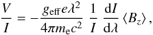 where V is the Stokes
parameter that measures the circular polarisation, I is the intensity in
the unpolarised spectrum, geff is the effective Landé factor,
e is the electron charge, λ is the wavelength,
me the electron mass, c the speed of light,
dI/dλ is the derivative of Stokes I,
and ⟨Bz⟩ is the mean longitudinal magnetic
field.
where V is the Stokes
parameter that measures the circular polarisation, I is the intensity in
the unpolarised spectrum, geff is the effective Landé factor,
e is the electron charge, λ is the wavelength,
me the electron mass, c the speed of light,
dI/dλ is the derivative of Stokes I,
and ⟨Bz⟩ is the mean longitudinal magnetic
field.
The mean longitudinal magnetic field was measured either by using only the absorption hydrogen Balmer lines or by using the entire spectrum, including all available absorption lines. Our measurements, acquired over a few years, are presented in Table 6, together with the modified Julian dates of mid-exposure. A few weak field detections at a significance level higher than 3σ were achieved for each star. As the rotation periods for both stars are unknown, it is not possible at the present stage to conclude whether the variability of the magnetic field is caused by a rotational modulation.
With respect to the reliability of our FORS 2 measurements of rather weak longitudinal
magnetic fields, we note that the feasibility of such measurements in stars of different
mass and at different evolutionary stages using FORS 1/2 in spectropolarimetric mode has
been demonstrated by numerous studies during the last ten years. It has also been
confirmed by comparing measurements of the magnetic field for well-studied magnetic stars
with values from the literature. These stars have typically strong longitudinal magnetic
fields of the order of a few kG. What is not yet so well established are the measurements
of several calibrators with magnetic fields well below 1000 G. The FORS
V/I spectrum is deduced from four spectra: the two
spectra for the ordinary and extraordinary beams coming out of the Wollaston prism, taken
at two different settings of the retarder wave plate. They are combined using the
following equation: 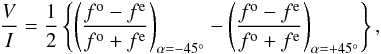 While
While  and
and
 , as well as
 and
and
 are taken at the same time, respectively,
this is obviously not true for the two pairs and leads to differences in flux levels.
Also, the transmission for the ordinary and extraordinary beams is not the same. In the
equation used for the determination of the V/I spectrum
above, both varying transmission and flux levels at different times are compensated
through the double difference, especially removing the need for a flatfield. Still, there
might be residuals left after using the above equation that come from instrumental
effects, e.g. crosstalk from linear to circular polarisation. The null spectrum is usually
determined as the difference between two consecutive V/I
spectra. This computation should get rid of the magnetic field signatures and leave only
the instrumental features. Yet, different S/Ns in the consecutive
V/I spectra might introduce spurious null signals.
are taken at the same time, respectively,
this is obviously not true for the two pairs and leads to differences in flux levels.
Also, the transmission for the ordinary and extraordinary beams is not the same. In the
equation used for the determination of the V/I spectrum
above, both varying transmission and flux levels at different times are compensated
through the double difference, especially removing the need for a flatfield. Still, there
might be residuals left after using the above equation that come from instrumental
effects, e.g. crosstalk from linear to circular polarisation. The null spectrum is usually
determined as the difference between two consecutive V/I
spectra. This computation should get rid of the magnetic field signatures and leave only
the instrumental features. Yet, different S/Ns in the consecutive
V/I spectra might introduce spurious null signals.
On the other hand, a few recent FORS 2 spectropolarimetric observations over the rotation/magnetic period of the bright classical Ap star HD 142070, with a weak magnetic field, typical for a number of objects observed with FORS 1/2, revealed a good agreement with the measurements obtained with a high-resolution spectropolarimeter (Mathys et al. 2012). These results indicate that the order of magnitude of the uncertainties achieved with FORS 2 is correct.
3. Results for individual targets
HD 11753: among the studied targets, the star HD 11753 with eleven HARPS observations has the best rotation phase coverage. This system is an SB1 with a period of 41.489 d, according to the 9th Catalogue of Spectroscopic Binary Orbits (Pourbaix et al. 2009). It is also an astrometric Hipparcos binary according to the CCDM catalogue (Dommanget & Nys 2002).
The spectra of HD 11753 exhibit a pronounced variability of Ti, Cr, Sr, and Y, and their surface inhomogeneous distribution was studied in detail by Briquet et al. (2010) and Makaganiuk et al. (2012). Results of Doppler imaging reconstruction using data sets separated by just a couple of weeks revealed the evolution of chemical spots already on such a short time scale (Briquet et al. 2010). The Doppler maps computed by Briquet et al. (2010) and Makaganiuk et al. (2012) are roughly consistent, showing strongly overabundant Y and Sr patches at the rotation phases 0.75–1.00 and lower abundance patches around the phases 0.10–0.40. The Ti and Cr patches show a more complex surface distribution, although the distribution of the most overabundant patches roughly resembles those of Y and Sr. Furthermore, a significant variation in the latitudinal element distribution and in the element abundance gradients is observed. Makaganiuk et al. (2012) assumed the time of the first night of observation as the zero phase, which corresponds to the rotation phase 0.42 in the work of Briquet et al. (2010). As we mention above, the rotation phases presented in Table 3 for the star HD 11753 were calculated following the ephemeris used by Briquet et al. (2010).
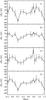 |
Fig. 1 Measurements of the mean longitudinal magnetic field as a function of the rotation phase for HD 11753. The measurements were carried out separately for the elements Ti, Cr, Fe, and Y (from bottom to top). Filled circles indicate 3σ measurements. |
The re-analysis of the HARPS spectra of this star by the moment technique using carefully selected line lists of the elements Ti, Cr, Fe, and Y shows remarkable results: the measurements on the Ti and Y lines reveal the presence of a weak negative magnetic field at the 3σ significance level at rotation phase 0.203, while the measurements on Cr and Fe show the presence of a weak positive magnetic field at the 3σ significance level at phase 0.783. Exactly at these rotation phases become the patches with the lowest surface element abundances as well as the patches with the highest surface element abundances best visible on the stellar surface. Even more striking is the behaviour of the longitudinal magnetic field over the stellar surface presented in Fig. 1. The measurements on all four elements indicate roughly the same kind of variability of the magnetic phase curve with predominantly negative field polarity at the location of the low-abundance patches and positive polarity at the location of the high-abundance patches. The behaviour of the magnetic field over the rotation cycle looks complex, indicating a non-sinusoidal character. It is also somewhat different for different elements and is very likely caused by differences in the surface abundance distribution for each element. Such a result is not unexpected since the lines of different elements with different abundance distributions across the stellar surface sample the magnetic field in different manners. Also, the presence of several element spots with different overabundances close to each other as presented in Fig. 8 in the work of Makaganiuk et al. (2012) for the Ti distribution indicates a more complex underlying magnetic field topology that cannot be represented by a simple dipole model. The presence of tangled magnetic fields on the surface of this star is strengthened by our 3σ detections of the mean quadratic magnetic field at two rotation phases, 0.413 and 0.993 (see Table 5) using Ti lines. As mentioned in the work of Makaganiuk et al. (2012), this element shows the most complex surface element distribution. In addition, a 3σ detection for positive crossover effect, 330 ± 108 km s-1 G, was achieved at the phase 0.832 for the sample of Ti lines, and for negative crossover effect, −467 ± 147 km s-1 G, at the phase 0.678 for the sample of Fe lines.
41 Eri: with a visual magnitude of 3.55 this SB2 system is one of the brightest targets among our stellar sample, with an excellent S/N achieved in the HARPS spectra. Four HARPS spectra were obtained for this star, but only three of them can be used for measurements because one observation was close to conjunction time, at MJD 55 201.77, where the lines of both components overlap in the spectra.
The atmospheric fundamental parameters for both components were studied by Dolk et al. (2003), who determined Teff = 12 750 K for the primary and Teff = 12 250 K for the secondary. Our inspection of the spectra belonging to the primary and the secondary reveal that the line profiles of several elements are clearly variable. Both components show typical HgMn peculiarities, but this is the first time that spectrum variability was also discovered in the spectra of the secondary component.
The problem of analysing the component spectra in double-lined spectroscopic binaries is a tough one, but fortunately several techniques for spectral disentangling have been developed in the past few years. In this work, we have applied the procedure of decomposition described in detail by González & Levato (2006). The resulting spectra were used to study the spectral variability of the components and the variation of radial velocities to improve the orbit of 41 Eri. We used all high-resolution spectra at our disposal obtained with FEROS, UVES, and HARPS, and lower-resolution (R = 20 000) EBASIM spectra. The ESO spectrographs UVES and FEROS are mounted on UT2 of the VLT at Paranal and at the 2.2 m telescope at La Silla, respectively. The EBASIM spectrograph is attached to the 2.1 m Jorge Sahade telescope at the CASLEO in Argentina. All measured radial velocities used to fit the orbit of this system are presented in Table 7, and the derived orbital parameters are listed in Table 8. In Fig. 2, we display the measured radial velocities together with the calculated orbital radial velocity curves. The orbit of the system 41 Eri is indistinguishable from a circular orbit. Thus, the solution presented in Table 8 corresponds to an orbit fitting with fixed value e = 0. If e is fitted as a free parameter, we determine the value e = 0.0001 ± 0.0019.
The projected equatorial rotation velocities were measured using the mean spectrum of each component obtained from the disentangling of HARPS spectra. The parameter v sin i was calculated for several unblended Fe ii and Cr ii lines through the measurement of the position of the first zero of the Fourier transform of the line profiles. In these calculations, the appropriate linear limb darkening coefficient for the corresponding stellar temperature and line wavelength was used. Since the orbit is circular and the time-scale for circularisation is longer than that for synchronisation, it can be assumed that the orbital motion and stellar rotation are already synchronised. The projected stellar radii and the measured v sin i-values for both components are presented in Table 8.
The error assigned to the stellar rotation is the standard error of the mean of the 25 lines measured and corresponds mainly to the random noise in the spectra. A more realistic estimate of the uncertainties should include other sources of error. We estimate that the influence of the instrumental profile is small, contributing with about 0.05 km s-1. However, the limb darkening adopted for the rotational profile is not well known, since its value may differ significantly from the continuum limb darkening. For this reason, we assume that errors below 1% for the rotational velocities are unrealistic and consequently adopted a 1% error in the stellar radii as a reasonable estimate.
In the disentangled spectra, the Hg ii line at λ3984 and the Fe ii lines appear to be stronger in the primary, while the Mn and Ti lines are stronger in the less massive star, i.e. in the component B. Since there is frequently confusion in the literature as to which component has to be considered as the primary and which as the secondary, we add the information on the spectrum appearance directly in both Tables 3 and 5, which present the magnetic field measurements.
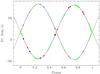 |
Fig. 2 Spectroscopic orbit of the system 41 Eri. Observations with FEROS are shown by red dots, with UVES by blue dots, with HARPS by black triangles, and with EBASIM by green symbols. Open symbols indicate the radial velocity measurements in the spectra of the secondary component, which is the less massive star. |
Orbital and fundamental parameters for the SB2 system 41 Eri.
Further, we used a mass-radius (M-R) diagram to estimate the inclination of the system and the absolute stellar parameters. In Fig. 3, we show the position of both components of 41 Eri in the M-R diagram for various possible values of orbital inclination, together with several isochrones and isotherms from stellar models by Schaller et al. (1992). Assuming Teff = 12 750 K for the primary and Teff = 12 250 K for the secondary (see e.g. Dolk et al. 2003), we obtain an inclination of 33.7°. The age of the system is estimated to be around 25–30 Myr, representing less than 10% of its main sequence life time.
We note that the system 41 Eri actually seems to be a triple one: Hubrig et al. (2001) studied this system with diffraction-limited
near-infrared ADONIS observations on La Silla and found a companion of
K = 9.9 at a distance of 532 and a position angle of 162.5°. This
finding was later confirmed by observations of Schöller et al. (2010) with NAOS-CONICA at the VLT.
The variability of the spectral lines was studied in the high-resolution disentangled spectra for each orbital phase. A distinct variability is observed for Hg, Ti, and Fe lines in the primary and for Hg, Mn, Ga, and Fe lines in the secondary. The profile variations of several lines over the rotation cycle are presented in Fig. 4. In the upper panel, we present the root mean square (rms) values of the residuals. The strongest rms peaks correspond to the Hg line in the spectra of the primary and to Mn and Ga lines in the spectra of the secondary component.
Since in both stars the line profiles belonging to several elements show significant variability, the disentangling process requires a dense high-resolution spectral time series. We note that even with the rather dense spectral time series obtained, the results are less reliable in spectral regions where both components exhibit variable line profiles. The analysis of the Mn line-profile variations in the secondary indicates that Mn is concentrated in a spot located on the stellar hemisphere opposite to the hemisphere facing the companion star. Around the orbital phase 0.5, i.e. the phase when the stellar surface facing the primary becomes better visible, the Mn lines appear significantly weaker. The Ga lines and the Hg ii line at λ3984 show qualitatively a very similar behaviour.
The distribution of the available measurements of the mean longitudinal magnetic field over the stellar surface in both components is presented in Fig. 5. As mentioned above, due to the overlap of spectral lines of components in one of the HARPS spectra, reliable results of the measurements can only be achieved at three rotation phases. 3σ detections were achieved using the sample of Ti lines in the spectra of the primary at the rotation phase 0.276 as well as the samples of Ti and Fe lines in the spectra of the secondary at the phase 0.673. An interesting fact discovered in these measurements is that the stellar surfaces with low-abundance element spots that face the companion star show negative magnetic field polarity, while for the opposite hemisphere covered by high abundance element spots, the magnetic field is positive.
A mean quadratic magnetic field at the 3σ level, 4520 ± 758 G, was detected in the primary at the phase 0.870 using the sample of Ti lines. As for the secondary, a quadratic magnetic field of 2332 ± 488 G and 2106 ± 634 G was detected at the phases 0.673 and 0.870, respectively, using the sample of Fe lines. Furthermore, we detect a quadratic magnetic field at a 3σ level, 3885 ± 1115 G at the phase 0.673, and a quadratic magnetic field 4484 ± 1201 G at the phase 0.870 using Ti lines. No crossover effect at a 3σ level was detected for this system.
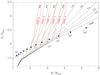 |
Fig. 3 Position of the components in the system 41 Eri in the mass-radius diagram for inclinations in the range 28−50° with a step of 2°. The red lines are isotherms interpolated in the stellar models. With Teff = 12 750 K for the primary and Teff = 12 250 K for the secondary, we obtain an inclination of 33.7°. Open circles indicate the position of the secondary component. |
 |
Fig. 4 Line-profile variations and the rms values in the spectra of both components of 41 Eri over the rotation period. The dotted line corresponds to the mean line profiles. The scales for the normalised flux have ticks of 0.1 in the lower panels and 0.01 in the upper panels, respectively. |
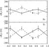 |
Fig. 5 Measurements of the mean longitudinal magnetic field as a function of the rotation phase for 41 Eri. The measurements were carried out separately for the elements Ti (bottom) and Fe (top). The solid line denotes the primary component, while the dashed line denotes the secondary component. Filled circles indicate 3σ measurements. |
66 Eri: ten HARPS polarimetric spectra were obtained over almost two orbital cycles of this SB2 system. Among them, one spectrum was taken close to the time of conjunction ii, at MJD 55 211.25, where the lines of both components overlap in the spectra. The most recent determination of fundamental and orbital parameters of 66 Eri was carried out by Makaganiuk et al. (2011a). In their work, however, there is a mismatch in the presentation of the orbital and fundamental parameters of the system, i.e. some parameters are ascribed to component A, while in actuality they belong to component B. We re-analysed 66 Eri using all spectroscopic material available to us: ten HARPS, four FEROS, and three UVES spectra. Furthermore, 18 spectra at a resolution of ~60 000 were obtained with the CORALIE echelle spectrograph, attached to the 1.2 m Leonard Euler telescope on La Silla in Chile. Additional radial velocity measurements were compiled from the literature. All these measurements for both the primary and the secondary component are presented in Tables 9 and 10. Similar to the study of 41 Eri, these radial velocity measurements were obtained as a result of spectral disentangling. As mentioned above, our phase zero for 66 Eri refers to the time of conjunction i, while the phase zero in the work of Makaganiuk et al. (2011a) refers to time of periastron. The time of conjunction is more useful because it refers to the position with respect to the companion, while the time of periastron is generally not well defined for binary systems with non-zero eccentricities. Furthermore, our MJD values are slightly different (by about 0.0012) from those presented by Makaganiuk et al. (2011b) because they are heliocentric and correspond to the middle of exposures.
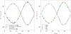 |
Fig. 6 Spectroscopic orbit of the system 66 Eri obtained using old data from the literature (left side) and new data consisting of ten HARPS, four FEROS, three UVES, and 18 CORALIE spectra (right side). Open symbols indicate the measurements of the secondary component, which is the less massive star. |
Orbital and fundamental parameters for the SB2 system 66 Eri.
In addition, we used the 83 old radial velocity measurements from Frost & Struve (1924). The orbital parameters are shown in Table 11. In Fig. 6, we present our calculated radial velocity curves along with the old and new radial velocity data.
Due to a rather large eccentricity of the system, e = 0.0844, the rotation period of 66 Eri is not expected to be the same as the orbital period. The period of corotation at periastron is 4.657 d, while the pseudo-synchronous period as defined by Hut (1981), is 5.3015 d. The latter is expected to correspond to the rotation period. Makaganiuk et al. (2011a) assumed the period of the orbital motion as the period of spectral variability, while our rotation phases presented in Table 3 adopt the pseudo-synchronisation period.
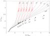 |
Fig. 7 Position of the components of 66 Eri in the M-R diagram for inclinations in the range 50−90° with a step of 2°. With Teff = 11 077 K for the primary and Teff = 10 914 K for the secondary, we obtain an inclination of 73.7°. Both components are located very close to the ZAMS. Open circles indicate the position of the secondary component. |
Similar to the procedure applied for 41 Eri, we used the M-R diagram to estimate the inclination of the system. Assuming Teff = 11 077 K for the primary and Teff = 10 914 K for the secondary (see e.g. Makaganiuk et al. 2011a), the system appears at an inclination of 73.7°. Figure 7 shows the position of the stellar components in the M-R diagram, where both companions are located very close to the zero age main sequence (ZAMS).
The presence of an additional companion in this system was reported from
diffraction-limited near-infrared observations. Hubrig et al. (2001) studied this system with the diffraction-limited near-infrared
ADONIS system on the ESO 3.6 m telescope and found a companion of K = 9.4
at a distance of 1613 and a position angle of 232.6°. The
presence of a companion was later confirmed by observations of Schöller et al. (2010) with NAOS-CONICA at the VLT.
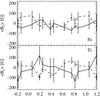 |
Fig. 8 Measurements of the mean longitudinal magnetic field as a function of the rotation phase for 66 Eri. The measurements were carried out separately for the elements Ti and Fe. The solid line denotes the primary component, while the dashed line denotes the secondary component. Filled circles indicate 3σ measurements. |
The quality of the polarimetric HARPS spectra is not as good as the spectra of HD 11753 and 41 Eri, with S/N mostly between 200 and 300. This could explain the larger inaccuracies in the magnetic field determinations and the fact that in our study only one detection at a 3σ significance level was achieved at the rotation phase 0.186 using Ti lines. The distribution of the mean longitudinal magnetic field values measured in both components over the rotation cycle is presented in Fig. 8. A comparison of the field distribution with the distribution of elements over the stellar surface presented in Fig. 7 in the work of Makaganiuk et al. (2011a) confirms the pattern already discovered in HD 11753 and 41 Eri: a negative mean longitudinal magnetic field is measured at the location of the lower abundance patches, i.e. on the stellar surface facing the companion, and the positive mean longitudinal magnetic field roughly corresponds to the location of the high-abundance patches located on the opposite hemisphere. A positive 3σ crossover, 1116 ± 374 km s-1 G, is observed in the sample of Fe lines in the primary at the phase 0.384. Using Fe lines in the secondary, we obtain a positive crossover 1795 ± 396 km s-1 G, at the phase 0.442. Furthermore, negative crossover, −1382 ± 450 km s-1 G, is observed in Fe lines in the primary at the phase 0.816. Interestingly, no significant crossover effect was found either in the primary or in the secondary using the sample of Ti lines. A mean quadratic magnetic field at the 3σ significance level was discovered in both components at several rotation phases using samples of Ti and Fe lines.
HD 33904: until now, four polarimetric observations have been obtained
with HARPS for this HgMn star, but only one observation was publically available in the ESO
archive at the time of our visitor stay at the ESO headquarters, which was aimed at the
reduction of the HARPS spectra with the HARPS pipeline machine. The spectral variability of
several elements was studied by Kochukhov et al. (2011), who also used the LSD technique with the mask covering 526 lines to
determine the longitudinal magnetic field and concluded that the upper limit for the field
in this star is only about 3 G. The available radial velocity data are not sufficient to
decide whether this star is a member of a SB system, but recent adaptive optics observations
by Schöller et al. (2010) presented the first direct
detection of a close companion candidate at a separation of
0352 and a position angle of 250.9°.
Measurements using the sample of Ti lines reveal that the mean quadratic magnetic field is
definitely present on the surface of this star, while the mean longitudinal magnetic field
measured on the same lines accounts for a 2.9σ detection.
Orbital and fundamental parameters for the eclipsing system AR Aur.
AR Aur: the eclipsing system AR Aur (HD 34364, B9V+B9.5V) with an orbital period of 4.13 d at an age of only 4 × 10⁶ yr belongs to the Aur OB1 association. Since its primary star of HgMn peculiarity is exactly on the ZAMS while the secondary is still contracting towards the ZAMS (e.g. Nordström & Johansen 1994), it presents the best case to study evolutionary aspects of the chemical peculiarity phenomenon. A presence of a third body in the system was discovered by Chochol et al. (1988). The existence of the as yet unseen third star with a mass of at least 0.51 M⊙ was inferred from a light-time effect in the observed minima with a period of 23.7 yr (Albayrak et al. 2003, see also Mikulášek et al. 2010). We re-determined the spectroscopic orbit of this triple system using all spectroscopic data available to us (21 SOFIN, 20 TLS, 26 STELLA, and nine UVES spectra). We also used the radial velocities measured by Folsom et al. (2010) for three ESPaDOnS and four NARVAL spectra. In these calculations, we adopted the binary period and parameters of the light-time orbit published by Albayrak et al. (2003) in order to account for the long-term variation of the center-of-mass velocity of the eclipsing pair and the light-time effect corrections to the epochs of observations. Radial velocity curves indicate that the eccentricity is indistinguishable from zero (e = 0.0009 ± 0.0011), in agreement with the photometric analysis of Nordström & Johansen (1994). We therefore adopted a circular orbit in our final calculations. The orbital parameters are listed in Table 12 and the radial velocity curve is shown in Fig. 9. It is clear from the lower panel of Fig. 9 that the influence of the third body cannot be neglected in the orbit fitting.
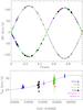 |
Fig. 9 Spectroscopic orbit of the eclipsing system AR Aur using SOFIN spectra obtained in 2002 and 2010 (blue squares), UVES spectra from 2005 (black dots), TLS-STELLA spectra from 2008/2009 (red triangles and green diamonds), three ESPaDOnS spectra (pluses), and four NARVAL spectra (stars). Open symbols indicate the measurements of the secondary component, which is the less massive star. The upper panel shows the velocity of the components of the eclipsing pair with respect to the center-of-mass of the binary; the lower panel shows the systemic velocity of the pair AB with respect to the center-of-mass of the triple system. |
The middle block of Table 12 corresponds to the results of the measurements of projected rotational velocities and the lower block to the combination of our spectroscopic orbit with the photometric inclination and relative radii of Nordström & Johansen (1994). According to these authors, the primary star, which is more massive and hotter, is slightly smaller than the secondary. However, the spectral lines of the secondary appear slightly narrower, which, assuming corotation, would suggest a smaller radius. The difference in vsini between both stars, however, is only marginal and, if real, could be explained by a non-uniform distribution of the elements Fe, Cr, and Ti with latitude. Variability of spectral lines associated with a large number of chemical elements was reported for the first time for the primary component of this eclipsing binary by Hubrig et al. (2006a). In the more recent study of this system by Hubrig et al. (2010), we presented the results of Doppler imaging for the reconstruction of the distribution of Fe and Y over the surface of the primary. We used a spectroscopic time series obtained in 2005 and from 2008 October to 2009 February. In the disentangling process, we adopted the photometric flux ratio obtained by Nordström & Johansen (1994), i.e. the light contributions of stars A and B to the continuum are adopted as 0.526 and 0.474, respectively. Our results showed a remarkable evolution of the elemental spot distribution and the overabundances. Measurements of the magnetic field with the moment technique using several elements revealed the presence of a longitudinal magnetic field of the order of a few hundred Gauss in both stellar components as well as a quadratic field of the order of 8 kG on the surface of the primary star.
To study the magnetic field geometry on the surface of the components in this system and its correlation with the surface inhomogeneous element distribution, a number of nights was allocated at the NOT in December 2010. However, due to bad weather conditions only five polarimetric observations were acquired for AR Aur. The distribution of the observations was fortunately rather random over the rotation/orbital period, allowing us to get an idea about the surface element distribution. The orbit of the system using all spectra of AR Aur available to us is presented in Fig. 9. The rotation phases were calculated using the ephemeris taken from the study of Albayrak et al. (2003).
In our analysis, similar to the analysis presented by Hubrig et al. (2010), we used the improved Doppler imaging code introduced by Freyhammer et al. (2009). This code utilises Tikhonov regularisation with a grid of 6 × 6° in a way similar to the Doppler imaging method described by Piskunov (2008). In the reconstruction, we searched for the minimum of the regularised discrepancy function, which includes the regularisation function and the discrepancy function describing the difference between observed and calculated line profiles. All atomic data in our analysis were taken from the VALD data base (Kupka et al. 1999). For the DI reconstruction, we selected the following lines belonging to the elements Fe, Sr, and Y: Fe ii 4923.9 Å, Sr ii 4215.5 Å, and Y ii 4900.1 Å. The computed Doppler maps in Mercator and spherical projections based only on five different rotation phases are presented in Fig. 10.
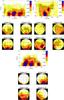 |
Fig. 10 Maps of the abundance distribution for Fe (top left), Sr (top right), and Y (bottom) on the surface of the primary in the system AR Aur. |
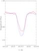 |
Fig. 11 Line profiles of the Sr ii 4215.5 Å line around rotation phase 0.68 for all available data sets between 2002 and 2010. The thick red continuous line refers to observations with SOFIN in 2010, the blue continuous line to those with UVES in 2005, the dashed line corresponds to observations at the Thüringer Landessternwarte and STELLA, and the dotted line corresponds to observations with SOFIN in 2002. |
Clearly, due to the low number of observations these maps cannot be used to study the evolution of element distribution over the stellar surface, but they allow us a rough estimate of the location of regions with element overabundances. Similar to previous maps obtained for AR Aur, we again find that the regions with lower abundances of Y and Sr are located on the stellar surface facing the companion, while spots with Y and Sr high abundances appear on the opposite hemispheres. Presently we have at our disposal four spectroscopic data sets obtained between 2002 and December 2010. The temporal evolution of chemical inhomogeneities is presented in Fig. 11, using as an example the profile variations of the Sr ii 4215.5 Å line. All four sets contain spectra at almost the same rotation phases, 0.68. The line profiles of Sr ii 4215.5 Å observed at this phase in all sets show that the Sr spots definitely changed their shape and abundance with time (see Fig. 11). The lowest Sr abundance appeared to be in December 2010, while the strongest Sr overabundance was observed in 2005.
In our magnetic field analysis, the longitudinal magnetic field strength measured in AR Aur is larger than that measured in other targets. However, due to the much lower resolution of the SOFIN spectra compared with the HARPS spectra and the not very high S/N, our measurement accuracies are poorest among the values presented in Table 3. At present, it is not clear to us whether the stronger magnetic field in this system can be explained by the aspect effect, if we assume that the field topology is characterised by the presence of magnetic regions predominantly in the vicinity of stellar equators. Since the AR Aur system is an eclipsing binary, it is the only system in our sample that offers the observer the best visibility of the surface equatorial regions. In any case, this system is one of the most promising targets to constrain the magnetic field topology in binaries with late B-type primaries. 3σ longitudinal magnetic field detections were achieved for measurements using Ti, Fe, and Y lines in the spectra of the primary in the phases 0.687 and 0.908 as well as for measurements using Fe lines in the spectra of the secondary at the phase 0.030. The variations of the mean longitudinal magnetic field in both components over the rotation cycle presented in Fig. 12 display a characteristic behaviour similar to that found for the binary stars discussed above. The mean quadratic magnetic field is detected at three different rotation phases in the primary.
HD 53244: the SB nature of this target was suggested by Schneider (1981). Schöller et al. (2010) found a companion candidate to this star at a separation of
0332 and a position angle of 114.8°. The
rotation period of HD 53244, P = 6.16 d, was derived by Briquet et al.
(2010) from the study of the variations of radial
velocities and equivalent widths of spectral lines belonging to the inhomogeneously
distributed elements Hg and Mn. However, Y lines appear extremely weak. No mean longitudinal
magnetic field was detected using the single HARPS observation of this star. A negative
crossover effect at the 3σ significance level,
−4073 ± 1118 km s-1 G, was detected using the sample of Cr lines.
κ Cnc: this system is an SB2 with a period of 6.3933 d,
according to the 9th Catalogue of Spectroscopic Binary Orbits (Pourbaix et al. 2009). Mason et al. (2001) found a companion on Besselian year 1999.1606 at a separation of
0286 and a position angle of 108°. This star
was also resolved by Roberts et al. (2005) on
Besselian year 2003.0077 with a separation of 030 and a position angle of 104°. Schöller
et al. (2010) detected this companion at a separation
of 0269 and a position angle of 109.7°.
Two HARPS polarimetric spectra of this system are available in the ESO archive. The detection of very faint spectral lines of the secondary in both spectra allowed us to determine the mass ratio, q = 0.490 ± 0.003. Combining our spectroscopic mass ratio with the orbital parameters P, e, and KA of the published SB1 orbit by Aikman (1976), we obtain MA sin3 i = 3.74 ± 0.13 M⊙ and MB sin3 i = 1.83 ± 0.04 M⊙. To learn about the nature of the secondary component and measure its rotational velocity, we applied spectral disentangling. The obtained secondary spectrum is consistent with a mid-A spectral type, which contributes only 7% to the total light of the system at λ5000. Since most lines in the spectrum of the secondary component are blended, the rotation velocity was determined using the technique developed by Díaz et al. (2011). As a result, we obtain vsini = 42.3 ± 1.5 km s-1. The primary star presents very narrow spectral lines with the vsini-value below 5 km s-1. Both components rotate asynchronously. In fact, according to estimates of their radii, the vsini values for pseudo-synchronisation for stars A and B are about 33 and 14 km s-1, respectively, and thus very far from the observed values.
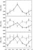 |
Fig. 12 Measurements of the mean longitudinal magnetic field presented as a function of the rotation phase for AR Aur. They were carried out separately for the elements Ti, Fe, and Y (from bottom to top). The solid line denotes the primary component, while the dashed line denotes the secondary component. Filled circles indicate 3σ measurements. |
With an orbital period of 6.39 d, the orbital phase difference between the two HARPS observations is 0.41. The strongest lines in the spectra belong to the elements Mn and Fe, while Y lines are extremely weak. The weak negative longitudinal magnetic field is detected at the 3σ significance level in the HARPS spectrum obtained at MJD 55 202.304 using Fe lines. Also, measurements using Mn lines resulting in ⟨Bz⟩ = −47 ± 15 G confirm the presence of a weak negative magnetic field at this epoch. No significant detection was achieved for the crossover effect and the quadratic magnetic field.
HD 101189: this target is not known to belong to a SB system. Schöller
et al. (2010) found a close companion candidate to
HD 101189 at a separation of 0337 and a position angle of 104.1°.
The first HARPS spectropolarimetric observation of this star was carried out at MJD 54982.4744, and its analysis was reported by Hubrig et al. (2011). For the same HARPS observations, Makaganiuk et al. (2011b) reported a non-detection with ⟨Bz⟩ = −95 ± 66 G using the LSD technique. The quality of the spectra obtained at this epoch was especially poor, with achieved S/N between 12 and 52. The measurements of Hubrig et al. delivered the same magnetic field (of the order of −200 G) for both the regular science Stokes V observations and the null spectrum. As the authors showed in their Fig. 8, this is because the spectrum with the best S/N (52 in that case) significantly contributes to the null spectrum. This result implies that if the observations are carried out with low S/N, and the difference in S/N in the sub-exposures is large, the magnetic field cannot be measured conclusively, and there is no use in the null spectrum to prove whether or not the detected field is real.
The second HARPS observation of HD 101189 was obtained on MJD 55201.3629. For this observation, we detect a weak magnetic field at the 3σ level ⟨Bz⟩ = −74 ± 24 G using Ti lines and ⟨Bz⟩ = −37 ± 11 G using Y lines. A quadratic field at 3σ significance level was detected for all line samples apart from the sample of Y lines. The shape of the line profiles of different elements is very different: Y lines appear double with two absorption maxima in the line profiles, while this profile shape is not observed in Mn, Fe, Cr, and Ti lines, suggesting a different spot distribution of these elements over the stellar surface. Only for the sample of Y lines do we observe the presence of a weak positive crossover effect, 764 ± 338 km s-1 G, at the 2.3σ level.
HD 221507: this target is not known to belong to a SB system. Hubrig
et al. (2001) studied this target with ADONIS and did
not detect any companion. However, Schöller et al. (2010) found a companion candidate to HD 221507 at a separation of
0641 and a position angle of 240.2°.
The rotation period of this star, P = 1.93 d was derived by Briquet et al. (2010) from the study of the variations of radial velocities and equivalent widths of spectral lines belonging to the inhomogeneously distributed elements Hg, Mn, and Y. We detect a weak longitudinal magnetic field at 3σ level ⟨Bz⟩ = 78 ± 25 G using Y lines. Also, measurements using Mn lines, ⟨Bz⟩ = 75 ± 23 G, show the presence of a positive longitudinal magnetic field. No significant crossover effect and quadratic magnetic field are detected in our measurements.
HD 179761 and HD 209459: the star HD 179761 is considered in the literature as a normal B-type star and HD 208459 as a superficially normal B-type star. Superficially normal B-type stars are generally indistinguishable from the normal stars in terms of their iron-peak elemental abundances (e.g. Smith & Dworetsky 1993). They are usually sharp-lined stars that possess normal MK classifications, but nonetheless exhibit mild peculiarities when observed at high spectral resolution.
Although HD 209459 is not a typical HgMn star, it is listed in the catalogue of HgMn stars by Schneider (1981). Our analysis of the HARPS spectropolarimetric material for this star indicates the absence of Hg and Y lines and the presence of weak Mn lines. The lines of Ti, Cr, and Fe appear rather strong and reveal a weak variability.
Ti, Cr, Mn, and Y lines are weak in the HARPS spectrum of HD 179761. We cannot report anything on the variability of this star as only a single HARPS observation is available.
Hubrig et al. (1999b) and Hubrig & Castelli (2001) used an anomalous strength of the Fe ii λ6147.7 line relative to the Fe ii λ6149.2 line in stars with magnetic fields to study the presence of magnetic fields in HgMn, normal, and superficially normal late-B type stars. In this method, previously introduced by Mathys (1990), the observed relative differences between the equivalent widths of the two Fe ii lines are compared with those derived from synthetic spectra computed by neglecting magnetic field effects. While the differences between the equivalent widths for HD 209459 were found to lie within the error limits, the differences for HD 179761 were found to be much larger, even if all observational and computational uncertainties are taken into account (Hubrig & Castelli 2001), which suggests the presence of a magnetic field in this star. Both HD 179761 and HD 209459 were also observed with FORS 1 at the VLT by Hubrig et al. (2006b), who reported a 3σ detection for the mean longitudinal magnetic field of HD 179761.
The observations with HARPS indicate the presence of a weak longitudinal magnetic field in HD 209459 at MJD 55417.149, measured using the samples of Ti, Cr, and Fe lines. A quadratic magnetic field of the order of 3 kG at the 3σ level was detected in HD 179761 using Fe lines, and much weaker quadratic fields of the order of 1.3–1.5 kG were detected in both observations of HD 209459 using Cr lines. The presence of a ~3 kG quadratic field in HD 179761 agrees well with the previous analysis of the relative magnetic intensification of the two Fe ii lines by Hubrig & Castelli (2001). We note that it is not the first time that a quadratic magnetic field is detected in upper main sequence stars considered as normal or superficially normal stars. Mathys & Hubrig (2006) studied the presence of a quadratic magnetic field in the superficially normal A-type star HD 91375. Their analysis led to the detection of a 1.7 kG quadratic field at a significance level of more than 4σ.
4. Discussion
The region of the main sequence centred on A and B stars, also referred to as the “tepid stars”, represents an ideal laboratory to study a wide variety of physical processes that are at work to a greater or lesser extent in most stellar types. These processes include radiation driven diffusion, differential gravitational settling, grain accretion, magnetic fields and non-radial pulsations. Understanding them is becoming increasingly important for the refinement of stellar evolution models and for the improved treatment of the stellar contribution in studies of galactic evolution. Presently, the radiative diffusion hypothesis developed by Michaud (1970) is the most frequently accepted theory for producing the observed anomalies in HgMn stars. According to Michaud et al. (1974), the effect of diffusion would cause a cloud of mercury to form high up in the HgMn star atmospheres. However, the impact of the radiative diffusion process has not yet been studied for any element considered in our work.
Based mostly on ESO/HARPS archive data, our analysis suggests the existence of intriguing correlations between magnetic field, abundance anomalies, and binary properties. In the SB2 systems with the synchronously rotating components, 41 Eri and AR Aur, the stellar surfaces facing the companion star usually display low-abundance element spots and negative magnetic field polarity. The surface of the opposite hemisphere, as a rule, is covered by high-abundance element spots and the magnetic field is positive at the rotation phases of the best-spot visibility. Also, Measurement results for the SB1 system HD 11753 indicate that element underabundance (respectively overabundance) is observed where the polarity of the magnetic field is negative (respectively positive). In the case of the very young pseudosynchronously rotating system 66 Eri, additional future observations are urgently needed to determine the period of the spectral variability and to investigate the presence of element-spot evolution. It is quite possible that because the system is not yet synchronised, a dynamical spot evolution is more pronounced compared to synchronised systems.
Although only rather weak longitudinal magnetic fields are detected on the surface of our targets, the numerous 3σ detections of mean quadratic magnetic fields strongly suggest that magnetic fields are present in their atmospheres. We note again the advantage of carrying out quadratic magnetic field measurements as they provide measurements of the magnetic field strength that are somewhat insensitive to the magnetic field structure, and especially suited for magnetic fields with complex structure.
The interactions of differential rotation, magnetic fields, and meridional flows in a tidal potential may lead to processes that can explain complex surface patterns. Possible instabilities should be studied by non-linear, three-dimensional simulations. The resulting fluctuations in velocity and magnetic field may not only explain the relatively small scales of surface magnetic fields, but also provide enhanced transport of angular momentum that explain the high rates of synchronisation. Synchronisation in an orbit with about 5 d period, an initial rotation period of 1 d, and stellar parameters similar to 66 Eri is roughly 104 times the dissipation time scale in the star (Zahn 2008). In a non-turbulent, non-magnetic star where only the microscopic gas viscosity can couple the surface with the interior, it would be impossible to reach synchronisation within the age of the universe. There are also gravity waves that lead to synchronisation, but for stars of 2–3 solar masses, this effect still takes roughly 109 years. Large-scale magnetic fields or turbulence can provide enough coupling to reach (pseudo-)synchronisation in about a million years.
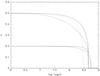 |
Fig. 13 Circularisation times for 41 Eri (dotted lines), 66 Eri (solid lines), and AR Aur (dashed lines), assuming that they formed with eccentric orbits with e0 = 0.2 and 0.5. |
As an illustration, we calculated the circularisation times for the systems 41 Eri, 66 Eri, and AR Aur, assuming that they formed with eccentric orbits. With the present parameters of the stars, the circularisation time scales, (− dlne/dt)-1 could be as high as 1010 yr. As they evolve within the main sequence, circularisation becomes more efficient, but even so they will arrive at the terminal age main sequence (TAMS) with a significant fraction of their original eccentricity: e/e0 = 0.15–0.70, depending on the original eccentricity e0. Figure 13 shows the evolution of e for the three systems, starting from e0 = 0.2 and 0.5. The solid line corresponds to 66 Eri, the dotted line to 41 Eri, and the dashed line to AR Aur. The vertical end of the curves to the right mark the TAMS. The calculations were performed using the stellar models calculated by Claret (2004), which include the internal structure constants required to calculate the orbital evolution. Considering that all three systems are young, with ages well below 108 yr, it would be expected that their present eccentricities woould not differ significantly from the original ones. The observed very low or null eccentricities cannot be explained as a consequence of standard tidal evolution.
The magneto-rotational instability is a candidate that can provide turbulence for a wide range of magnetic field strengths and field topologies, but only if the internal angular velocity of the star decreases with the distance from the rotation axis. Since synchronisation in the systems considered here is in fact a braking process, the star may exhibit a slower rotation near its surface than deeply inside. Numerical simulations should elucidate the expected enhancement of the viscosity in the star and will also deliver surface topologies of the fields resulting from this or other instabilities that can be compared to the observed patterns.
Tidal forces strongly depend on the distance between the components. For the three SB2
systems with synchronised and pseudosynchronised components, 41 Eri, 66 Eri, and AR Aur, we
estimated the fractional radii
rj = Rj/a.
Assuming for 41 Eri 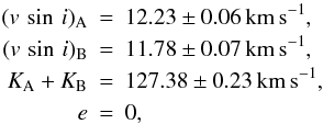 it follows that
RA/r = 0.096 ± 0.001 and
RB/r = 0.093 ± 0.001.
it follows that
RA/r = 0.096 ± 0.001 and
RB/r = 0.093 ± 0.001.
If we assume for 66 Eri pseudosynchronisation (Prot = 5.3015 d), we obtain RA/r = 0.084 ± 0.001 and RB/r = 0.080 ± 0.001.
For AR Aur we use 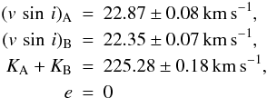 and obtain
RA/a = 0.102 ± 0.001 and
RB/a = 0.099 ± 0.001.
and obtain
RA/a = 0.102 ± 0.001 and
RB/a = 0.099 ± 0.001.
Since the fractional radii in these systems are quite large, the components in the close binary systems are subject to tidal forces acting differentially throughout their bodies and causing various effects in the system. The tidal effects include synchronisation of the rotational periods with the orbital period, circularisation of the orbit, and alignment of the rotation axes with the orbital axis. All these changes in the dynamical properties of the stars happen on different time scales. The spin-down may be a surface effect, but the star then possesses an internal differential rotation that may lead to hydrodynamic or magnetohydrodynamic instabilities. Even a moderately turbulent state generated by an instability will lead to much stronger coupling with the stellar interior and redistribute angular momentum.
To establish the evolutionary status of the HgMn stars in our sample, we studied their distribution in the H-R diagram. To this aim, the distances were calculated mainly using Hipparcos parallaxes (van Leeuwen 2007). For stars with high galactic latitudes, we estimated the interstellar absorption using Schlegel et al. (1998) maps and the distance by applying the same procedure as Bilir et al. (2008). Since this approach is not valid for targets located very close to the galactic plane, we estimated the absorption in a different way for the low-latitude stars HD 101189 and AR Aur. HD 101189 is located in the field of the open cluster NGC 3766, but it is a foreground star. This fact allowed us to estimate the absorption to the star using cluster reddening and the distance ratio. For the eclipsing binary AR Aur, we adopted the absolute stellar parameters derived by Nordstrom & Johansen (1994) from light and radial velocity curves. The star HD 65949, which is the faintest and most distant star, belongs to the open cluster NGC 2516. We used, therefore, the cluster distance and reddening published by Terndrup et al. (2002) to obtain absolute magnitude and intrinsic color. In the case of double-lined spectroscopic binaries, the position of the individual components in the H-R diagram was calculated using the spectroscopic mass ratio, from which the magnitude difference between the components was estimated by interpolating in the Geneva stellar models (Schaller et al. 1992). Figure 14 shows the position of the 11 HgMn stars in the color-magnitude diagram, together with isochrones taken from Schaller et al. (1992). Six stars in our sample, 41 Eri A, 41 Eri B, 66 Eri A, AR Aur A, HD 65949, and HD 221507, are located very close to the ZAMS.
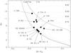 |
Fig. 14 H-R diagram for the HgMn stars in our sample. Continuous lines present the ZAMS and TAMS. Dotted lines present isochrones for log (t) from 7.00 to 8.70. |
From the knowledge of orbital parameters, fundamental parameters of components, and fractional radii, it is possible to estimate the reflection effect, gravitational distortion, and darkening for a typical HgMn star in a SB2 system. One of the consequences of the proximity of the stars is the departure from sphericity of the stellar surface. The star acquires a somewhat larger dimension along the line passing through the two star centres, while it has a smaller radius in the direction that is perpendicular to the former line and also lies in the orbital plane. The relative differences between both radii are 0.09% and 0.08% for the two components of the system 41 Eri, 0.05% and 0.06% for the system 66 Eri, and 0.09% and 0.10% for the system AR Aur. Observational effects of such stellar shapes are, for example, the variation of the vsini-value, which in the three systems studied is below the observational errors, and light variations due to the variation of the stellar disk size, which is expected to be of the order of 2–3 mmag. An effect that could affect physical conditions in the stellar atmosphere is the reflection effect. Assuming an albedo equal to 1 (the usual assumption for stars with radiative envelopes) and the temperatures and geometrical configuration of each system, we estimate that the temperature excess in the surface region facing the companion is between 20 and 40 K, which represents 0.18–0.38% of the star temperature. The question to solve is whether such small temperature differences can be considered a reasonable explanation of the origin of the low- and high-abundance spots observed either on the surface facing the companion or on the surface hidden to the companion. Although it is currently not easy to give an answer without a specific model of time-dependent diffusion processes, it seems very unlikely that these processes are the main cause of the observed abundance pattern. We note that the early circularisation and a very specific configuration of chemical spots in binary systems support the idea of an important impact of magnetic fields on the physical processes taking place in these stars. Since the orbital parameters of close binaries can change as a consequence of the action of tidal forces or other mechanisms, the influence of the presence of a stellar companion on the physical processes playing a role in the formation of chemical anomalies is expected to vary with time. The atmospheric physical conditions for the development of chemical inhomogeneities might appear favourable at certain stages of the stellar life and unfavourable at other stages.
Further studies using high S/N circularly polarised spectra well-distributed throughout the rotation period of a representative sample of HgMn spectroscopic binaries sampling a wide range of inclinations of the rotation axis to the line of sight are urgently needed to map their magnetic field and elemental abundances with a Zeeman-Doppler imaging code. The sampling of a wide range of inclination of the rotation axis to the line of sight in HgMn systems is especially important because the latitudinal information on the surface abundance distribution of different elements in HgMn stars is still rather poor. In this way, it will be possible to probe correlations between the binary properties, the magnetic field structure, and the abundance inhomogeneities. At the same time, we will be able to gain insight into the mechanisms responsible for the chemical inhomogeneities and their dynamical evolution on the surface of HgMn stars.
Online material
Logbook of the spectropolarimetric observations.
Measurements of the mean longitudinal magnetic field using sets of lines belonging to different elements.
Line lists for the different elements used in the magnetic field measurements.
Measurements of the quadratic magnetic field using sets of lines belonging to different elements.
Magnetic field measurements of HD 19400 and HD 65949 using FORS 1/2.
Radial velocity measurements carried out for the primary and secondary components in the SB2 system 41 Eri.
Measurements of radial velocities for the primary and secondary component of the SB2 system 66 Eri.
Measurements of radial velocities for the primary and secondary component of the SB2 system 66 Eri, taken from the literature.
The spectropolarimetric capabilities of FORS 1 were moved to FORS 2 in 2009.
Acknowledgments
We are grateful to G. Mathys for valuable discussions and to the anonymous referee for useful comments. This research made use of the SIMBAD database, operated at CDS, Strasbourg, France. H.K. acknowledges the support from the European Commission under the Marie Curie IEF Programme in FP7. Nordic Optical Telescope is operated on the island of La Palma jointly by Denmark, Finland, Iceland, Norway, and Sweden, in the Spanish Observatorio del Roque de los Muchachos of the Instituto de Astrofisica de Canarias.
References
- Abt, H. A., & Snowden, M. S. 1973, ApJS 25, 137 [NASA ADS] [CrossRef] [Google Scholar]
- Abt, H. A., Chaffee, F. H., & Suffolk, G. 1972, ApJ, 175, 779 [Google Scholar]
- Adelman, S. J., Gulliver, A. F., Kochukhov, O., & Ryabchikova, T. 2002, ApJ, 575, 449 [NASA ADS] [CrossRef] [Google Scholar]
- Aikman, G. C. L. 1976, Publ. Dominion Astrophys. Obs., 14, 379 [Google Scholar]
- Albayrak, B., Ak, T., & Elmasli, A. 2003, AN, 324, 523 [NASA ADS] [Google Scholar]
- Alonso, M. S., López-García, Z., Malaroda, S., & Leone, F. 2003, A&A, 402, 331 [NASA ADS] [CrossRef] [EDP Sciences] [Google Scholar]
- Bilir, S., Ak, T., Soydugan, E., et al. 2008, AN, 329, 835 [Google Scholar]
- Briquet, M., Korhonen, H., González, J. F., et al. 2010, A&A, 511, A71 [NASA ADS] [CrossRef] [EDP Sciences] [Google Scholar]
- Bychkov, V. D., Bychkova, L. V., & Madej, J. 2009, MNRAS, 394, 1338 [Google Scholar]
- Castelli, F., & Hubrig, S. 2004a, A&A, 425, 263 [NASA ADS] [CrossRef] [EDP Sciences] [Google Scholar]
- Castelli, F., & Hubrig, S. 2004b, A&A, 421, L1 [NASA ADS] [CrossRef] [EDP Sciences] [Google Scholar]
- Catanzaro, G., & Leto, P. 2004, A&A, 416, 661 [NASA ADS] [CrossRef] [EDP Sciences] [Google Scholar]
- Chochol, D., Juza, K., Zverko, J., et al. 1988, Bull. Astr. Inst. Czechoslovakia, 39, 69 [NASA ADS] [Google Scholar]
- Claret, A. 2004, A&A, 424, 919 [NASA ADS] [CrossRef] [EDP Sciences] [Google Scholar]
- Cowley, C. R., Hubrig, S., Palmeri, P., et al. 2010, MNRAS, 405, 1271 [NASA ADS] [Google Scholar]
- Díaz, C. G., González, J. F., Levato, H., & Grosso, M. 2011, A&AS, 531, A143 [NASA ADS] [CrossRef] [EDP Sciences] [Google Scholar]
- Dolk, L., Wahlgren, G. M., & Hubrig, S. 2003, A&A, 402, 299 [NASA ADS] [CrossRef] [EDP Sciences] [Google Scholar]
- Dommanget, J., & Nys, O. 2002, CCDM (Catalog of Components of Double & Multiple stars) [Google Scholar]
- Donati, J.-F., Semel, M., Carter, B. D., et al. 1997, MNRAS, 291, 658 [NASA ADS] [CrossRef] [MathSciNet] [Google Scholar]
- Folsom, C. P., Kochukhov, O., Wade, G. A., et al. 2010, MNRAS, 407, 2383 [NASA ADS] [CrossRef] [Google Scholar]
- Freyhammer, L. M., Kurtz, D. W., Elkin, V. G., et al. 2009, MNRAS, 396, 325 [NASA ADS] [CrossRef] [Google Scholar]
- Frost, E. B., & Struve, O. 1924, ApJ, 60, 313 [NASA ADS] [CrossRef] [Google Scholar]
- González, J. F., & Levato, H. 2006, A&A, 448, 283 [NASA ADS] [CrossRef] [EDP Sciences] [Google Scholar]
- Hubrig, S., & Castelli, F. 2001, A&A, 375, 963 [NASA ADS] [CrossRef] [EDP Sciences] [Google Scholar]
- Hubrig, S., & Mathys, G. 1995, Comments Astrophys., 18, 167 [Google Scholar]
- Hubrig, S., Castelli, F., & Mathys, G. 1999a, A&A, 341, 190 [NASA ADS] [Google Scholar]
- Hubrig, S., Castelli, F., & Wahlgren, G. M. 1999b, A&A, 346, 139 [NASA ADS] [Google Scholar]
- Hubrig, S., Le Mignant, D., North, P., & Krautter, J. 2001, A&A, 372, 152 [NASA ADS] [CrossRef] [EDP Sciences] [Google Scholar]
- Hubrig, S., Kurtz, D. W., Bagnulo, S., et al. 2004a, A&A, 415, 661 [NASA ADS] [CrossRef] [EDP Sciences] [Google Scholar]
- Hubrig, S., Szeifert, T., Schöller, M., et al. 2004b, A&A, 415, 685 [NASA ADS] [CrossRef] [EDP Sciences] [Google Scholar]
- Hubrig, S., González, J. F., Savanov, I., et al. 2006a, MNRAS, 371, 1953 [NASA ADS] [CrossRef] [Google Scholar]
- Hubrig, S., North, P., Schöller, M., & Mathys, G. 2006b, AN, 327, 289 [Google Scholar]
- Hubrig, S., Savanov, I., Ilyin, I., et al. 2010, MNRAS, 408, L61 [NASA ADS] [CrossRef] [Google Scholar]
- Hubrig, S., González, J. F., Ilyin, I., et al. 2011, AN, 332, 998 [Google Scholar]
- Hut, P. 1981, A&AS, 99, 126 [NASA ADS] [Google Scholar]
- Ilyin, I. 2000, Ph.D. Thesis, University of Oulu, Finland [Google Scholar]
- Ilyin, I. 2012, AN, 333, 213 [Google Scholar]
- Kochukhov, O., Adelman, S. J., Gulliver, A. F., & Piskunov, N. 2007, Nature Phys., 3, 526 [Google Scholar]
- Kochukhov, O., Makaganiuk, V., Piskunov, N., et al. 2011, A&A, 534, L13 [NASA ADS] [CrossRef] [EDP Sciences] [Google Scholar]
- Kupka, F., Piskunov, N., Ryabchikova, T. A., et al. 1999, A&AS, 138, 119 [NASA ADS] [CrossRef] [EDP Sciences] [MathSciNet] [PubMed] [Google Scholar]
- Kurucz, R. L. 1989, http://kurucz.cfa.harvard.edu/atoms [Google Scholar]
- Maitzen, H. M. 1984, A&A, 138, 493 [NASA ADS] [Google Scholar]
- Makaganiuk, V., Kochukhov, O., Piskunov, N., et al. 2011a, A&A, 529, A160 [NASA ADS] [CrossRef] [EDP Sciences] [Google Scholar]
- Makaganiuk, V., Kochukhov, O., Piskunov, N., et al. 2011b, A&A, 525, A97 [NASA ADS] [CrossRef] [EDP Sciences] [Google Scholar]
- Makaganiuk, V., Kochukhov, O., Piskunov, N., et al. 2011c, A&A, 534, L13 [NASA ADS] [CrossRef] [EDP Sciences] [Google Scholar]
- Makaganiuk, V., Kochukhov, O., Piskunov, N., et al. 2012, A&A, 539, A142 [NASA ADS] [CrossRef] [EDP Sciences] [Google Scholar]
- Mason, B. D., Hartkopf, W. I., Holdenried, E. R., & Rafferty, T. J. 2001, AJ, 121, 3224 [NASA ADS] [CrossRef] [Google Scholar]
- Mathys, G. 1988, A&A, 189, 179 [NASA ADS] [Google Scholar]
- Mathys, G. 1990, A&A, 232, 151 [NASA ADS] [Google Scholar]
- Mathys, G. 1991, A&AS, 89, 121 [NASA ADS] [Google Scholar]
- Mathys. G. 1993, in Peculiar versus Normal Phenomena in A-type and Related Stars, eds. M. M. Dworetsky, F. Castelli, & R. Faraggiana (San Francisco: ASP), ASP Conf. Ser., 44, 232 [Google Scholar]
- Mathys, G. 1995a, A&A, 293, 733 [NASA ADS] [Google Scholar]
- Mathys, G. 1995b, A&A, 293, 746 [NASA ADS] [Google Scholar]
- Mathys, G., & Hubrig, S. 1995, A&A, 293, 810 [NASA ADS] [Google Scholar]
- Mathys, G., & Hubrig, S. 2006, A&A, 463, 699 [NASA ADS] [CrossRef] [EDP Sciences] [Google Scholar]
- Mathys, G., Hubrig, S., Mason, E., et al. 2012, AN, 333, 30 [Google Scholar]
- Mayor, M., Pepe, F., Queloz, D., et al. 2003, The ESO Messenger, 114, 20 [Google Scholar]
- Michaud, G. 1970, ApJ, 160, 641 [NASA ADS] [CrossRef] [Google Scholar]
- Michaud, G., Reeves, H., & Charland, Y. 1974, A&A, 37, 313 [NASA ADS] [Google Scholar]
- Mikulášek, Z., Žižnovský, J., Hubrig, S., et al. 2010, in Binaries – Key to Comprehension of the Universe, eds. A. Prša & M. Zejda (San Francisco: ASP), ASP Conf. Ser., 435, 337 [Google Scholar]
- Nordström, B., & Johansen, K. T. 1994, A&A, 282, 787 [NASA ADS] [Google Scholar]
- Nuñez, N. E., González, J. F., & Hubrig, S. 2011, Proc. Conf. Magnetic Stars. August 27–September 01, 2010, Special Astrophysical Observatory, Russia, eds. I. I. Romanyuk, & D. O. Kudryavtsev, 361 [Google Scholar]
- Piskunov, N. 2008, Phys. Scripta, 133, 014017 [CrossRef] [Google Scholar]
- Pourbaix, D., Tokovinin, A. A., Batten, A. H., et al. 2009, A&A, 424, 727 [Google Scholar]
- Renson, P., & Manfroid, J. 2009, A&A, 498, 961 [NASA ADS] [CrossRef] [EDP Sciences] [Google Scholar]
- Roberts, L. C., Jr., Turner, N. H., Bradford, L. W., et al. 2005, AJ, 130, 2262 [NASA ADS] [CrossRef] [Google Scholar]
- Schaller, G., Schaerer, D., Meynet, G., & Maeder, A. 1992, A&A, 96, 269 [Google Scholar]
- Schlegel, D. J., Finkbeiner, D. P., & Davis, M. 1998, ApJ, 500, 525 [NASA ADS] [CrossRef] [Google Scholar]
- Schneider, H. 1981, A&AS, 44, 137 [NASA ADS] [Google Scholar]
- Schöller, M., Correia, S., Hubrig, S., & Ageorges, N. 2010, A&A, 522, A85 [NASA ADS] [CrossRef] [EDP Sciences] [Google Scholar]
- Smith, K. C., & Dworetsky, M. M. 1993, A&A, 274, 335 [NASA ADS] [Google Scholar]
- Snik, F., Kochukhov, O., Piskunov, N., et al. 2011, in Solar Polarization 6, eds. J. R. Kuhn, D. M. Harrington, H. Lin, et al. (San Francisco: ASP), ASP Conf. Ser., 437, 237 [Google Scholar]
- Terndrup, D. M., Pinsonneault, M., Jeffries, R. D., et al. 2002, ApJ, 576, 950 [NASA ADS] [CrossRef] [Google Scholar]
- Tuominen, I., Ilyin, I., & Petrov, P. 1999, in Astrophysics with the NOT, eds. H. Karttunen, & V. Piirola, University of Turku, Tuorla Observatory, 47 [Google Scholar]
- van Leeuwen, F. 2007, A&A, 474, 653 [NASA ADS] [CrossRef] [EDP Sciences] [Google Scholar]
- Wahlgren, G. M., Ilyin, I., & Kochukhov, O. 2001, A&AS, 19913504 [Google Scholar]
- Wolff, S. C., & Wolff, R. J. 1974, ApJ, 194, 65 [NASA ADS] [CrossRef] [Google Scholar]
- Young, A. 1976, PASP, 88, 275 [NASA ADS] [CrossRef] [Google Scholar]
- Yushchenko, A. V., Gopka, V. F., Khokhlova, V. L., et al. 1999, Astron. Lett., 25, 453 [NASA ADS] [Google Scholar]
- Yushchenko, A. V., Gopka, V. F., Khokhlova, V. L., & Tomkin, J. 2001, IBVS, 5213, 1 [NASA ADS] [Google Scholar]
- Zahn, J.-P. 2008, eds. M.-J. Goupil, & J.-P. Zahn, EAS Publ. Ser., 29, 67 [Google Scholar]
All Tables
Measurements of the mean longitudinal magnetic field using sets of lines belonging to different elements.
Measurements of the quadratic magnetic field using sets of lines belonging to different elements.
Radial velocity measurements carried out for the primary and secondary components in the SB2 system 41 Eri.
Measurements of radial velocities for the primary and secondary component of the SB2 system 66 Eri.
Measurements of radial velocities for the primary and secondary component of the SB2 system 66 Eri, taken from the literature.
All Figures
|
Fig. 1 Measurements of the mean longitudinal magnetic field as a function of the rotation phase for HD 11753. The measurements were carried out separately for the elements Ti, Cr, Fe, and Y (from bottom to top). Filled circles indicate 3σ measurements. |
| In the text | |
|
Fig. 2 Spectroscopic orbit of the system 41 Eri. Observations with FEROS are shown by red dots, with UVES by blue dots, with HARPS by black triangles, and with EBASIM by green symbols. Open symbols indicate the radial velocity measurements in the spectra of the secondary component, which is the less massive star. |
| In the text | |
|
Fig. 3 Position of the components in the system 41 Eri in the mass-radius diagram for inclinations in the range 28−50° with a step of 2°. The red lines are isotherms interpolated in the stellar models. With Teff = 12 750 K for the primary and Teff = 12 250 K for the secondary, we obtain an inclination of 33.7°. Open circles indicate the position of the secondary component. |
| In the text | |
|
Fig. 4 Line-profile variations and the rms values in the spectra of both components of 41 Eri over the rotation period. The dotted line corresponds to the mean line profiles. The scales for the normalised flux have ticks of 0.1 in the lower panels and 0.01 in the upper panels, respectively. |
| In the text | |
|
Fig. 5 Measurements of the mean longitudinal magnetic field as a function of the rotation phase for 41 Eri. The measurements were carried out separately for the elements Ti (bottom) and Fe (top). The solid line denotes the primary component, while the dashed line denotes the secondary component. Filled circles indicate 3σ measurements. |
| In the text | |
|
Fig. 6 Spectroscopic orbit of the system 66 Eri obtained using old data from the literature (left side) and new data consisting of ten HARPS, four FEROS, three UVES, and 18 CORALIE spectra (right side). Open symbols indicate the measurements of the secondary component, which is the less massive star. |
| In the text | |
|
Fig. 7 Position of the components of 66 Eri in the M-R diagram for inclinations in the range 50−90° with a step of 2°. With Teff = 11 077 K for the primary and Teff = 10 914 K for the secondary, we obtain an inclination of 73.7°. Both components are located very close to the ZAMS. Open circles indicate the position of the secondary component. |
| In the text | |
|
Fig. 8 Measurements of the mean longitudinal magnetic field as a function of the rotation phase for 66 Eri. The measurements were carried out separately for the elements Ti and Fe. The solid line denotes the primary component, while the dashed line denotes the secondary component. Filled circles indicate 3σ measurements. |
| In the text | |
|
Fig. 9 Spectroscopic orbit of the eclipsing system AR Aur using SOFIN spectra obtained in 2002 and 2010 (blue squares), UVES spectra from 2005 (black dots), TLS-STELLA spectra from 2008/2009 (red triangles and green diamonds), three ESPaDOnS spectra (pluses), and four NARVAL spectra (stars). Open symbols indicate the measurements of the secondary component, which is the less massive star. The upper panel shows the velocity of the components of the eclipsing pair with respect to the center-of-mass of the binary; the lower panel shows the systemic velocity of the pair AB with respect to the center-of-mass of the triple system. |
| In the text | |
|
Fig. 10 Maps of the abundance distribution for Fe (top left), Sr (top right), and Y (bottom) on the surface of the primary in the system AR Aur. |
| In the text | |
|
Fig. 11 Line profiles of the Sr ii 4215.5 Å line around rotation phase 0.68 for all available data sets between 2002 and 2010. The thick red continuous line refers to observations with SOFIN in 2010, the blue continuous line to those with UVES in 2005, the dashed line corresponds to observations at the Thüringer Landessternwarte and STELLA, and the dotted line corresponds to observations with SOFIN in 2002. |
| In the text | |
|
Fig. 12 Measurements of the mean longitudinal magnetic field presented as a function of the rotation phase for AR Aur. They were carried out separately for the elements Ti, Fe, and Y (from bottom to top). The solid line denotes the primary component, while the dashed line denotes the secondary component. Filled circles indicate 3σ measurements. |
| In the text | |
|
Fig. 13 Circularisation times for 41 Eri (dotted lines), 66 Eri (solid lines), and AR Aur (dashed lines), assuming that they formed with eccentric orbits with e0 = 0.2 and 0.5. |
| In the text | |
|
Fig. 14 H-R diagram for the HgMn stars in our sample. Continuous lines present the ZAMS and TAMS. Dotted lines present isochrones for log (t) from 7.00 to 8.70. |
| In the text | |
Current usage metrics show cumulative count of Article Views (full-text article views including HTML views, PDF and ePub downloads, according to the available data) and Abstracts Views on Vision4Press platform.
Data correspond to usage on the plateform after 2015. The current usage metrics is available 48-96 hours after online publication and is updated daily on week days.
Initial download of the metrics may take a while.