| Issue |
A&A
Volume 547, November 2012
|
|
|---|---|---|
| Article Number | A81 | |
| Number of page(s) | 17 | |
| Section | Atomic, molecular, and nuclear data | |
| DOI | https://doi.org/10.1051/0004-6361/201219749 | |
| Published online | 31 October 2012 | |
Influence of collisional rate coefficients on water vapour excitation
1 Departamento de Astrofísica, Centro de Astrobiología, CSIC-INTA, Ctra. de Torrejón a Ajalvir km 4, 28850 Madrid, Spain
e-mail: This email address is being protected from spambots. You need JavaScript enabled to view it.
2 Observatoire de Paris, LUTH UMR CNRS 8102, 5 place Janssen, 92195 Meudon, France
3 Université Pierre et Marie Curie, LPMAA UMR CNRS 7092, Case 76, 4 place Jussieu, 75252 Paris Cedex 05, France
4 UJF-Grenoble 1/CNRS-INSU, Institut de Planétologie et d’Astrophysique de Grenoble (IPAG) UMR 5274, 38041 Grenoble, France
Received: 4 June 2012
Accepted: 7 January 1900
Abstract
Context. Water is a key molecule in many astrophysical studies that deal with star or planet forming regions, evolved stars, and galaxies. Its high dipole moment makes this molecule subthermally populated under the typical conditions of most astrophysical objects. This motivated calculation of various sets of collisional rate coefficients (CRC) for H2O (with He or H2), which are needed to model its rotational excitation and line emission.
Aims. The most accurate set of CRC are the quantum rates that involve H2. However, they have been published only recently, and less accurate CRC (quantum with He or quantum classical trajectory (QCT) with H2) were used in many studies before that. This work aims to underline the impact that the new available set of CRC have on interpretations of water vapour observations.
Methods. We performed accurate non-local, non-LTE radiative transfer calculations using different sets of CRC to predict the line intensities from transitions that involve the lowest energy levels of H2O (E < 900 K). The results obtained from the different CRC sets were then compared using line intensity ratio statistics.
Results. For the whole range of physical conditions considered in this work, we find that the intensities based on the quantum and QCT CRC are in good agreement. However, at relatively low H2 volume density (n(H2) < 107 cm-3) and low water abundance (χ(H2O) < 10-6), which corresponds to physical conditions relevant when describing most molecular clouds, we find differences in the predicted line intensities of up to a factor of ~3 for the bulk of the lines. Most of the recent studies interpreting early Herschel Space Observatory spectra have used the QCT CRC. Our results show that, although the global conclusions from those studies will not be drastically changed, each case has to be considered individually, since depending on the physical conditions, the use of the QCT CRC may lead to a mis-estimate of the water vapour abundance of up to a factor of ~3. Additionally, the comparison of the quantum state-to-state and thermalised CRC, including the description of the population of the H2 rotational levels, show that above TK ~ 100 K, large differences are expected from those two sets for the p–H2 symmetry. Finally, we find that at low temperature (i.e. TK < 100 K) modelled line intensities will be differentially affected by the symmetry of the H2 molecule. If a significant number of H2O lines is observed, it is then possible to obtain an estimate of the H2 ortho-to-para ratio from the analysis of the line intensities.
Key words: line: formation / molecular data / radiative transfer / radiation mechanisms: thermal / ISM: abundances / ISM: molecules
© ESO, 2012
1. Introduction
Water is a key molecule for both the chemistry and the cooling budget along the star formation trail. Determining the water vapour abundance is a long-standing problem in astrophysics. Because water vapour is predicted to be an abundant molecule in the gas phase, determining its spatial extent, its distribution, and its abundance is crucial for modelling the chemistry and the physics of molecular clouds, comets, evolved stars, and galaxies (Neufeld & Kaufman 1993; Neufeld et al. 1995; Cernicharo & Crovisier 2005; van Dishoeck et al. 2011). In warm molecular clouds, water vapour can play a critical role in the gas cooling (Neufeld & Kaufman 1993; Neufeld et al. 1995), hence in the evolution of these objects.
Unfortunately, water is an abundant molecule in our atmosphere, making it particularly difficult to observe its rotational lines and vibrational bands from Earth. Even so, some observations of H2O maser lines have been performed from ground-based and airborne telescopes: the 616 − 523 at 22 GHz (Cheung et al. 1969), the 515 − 422 at 325 GHz (Menten et al. 1990a), the 1029 − 936 at 321 GHz (Menten et al. 1990b), and the 313 − 220 at 183.31 GHz (Waters et al. 1980; Cernicharo et al. 1990, 1994). The spectrometers on board the Infrared Space Observatory (Kessler et al. 1996) provided a unique opportunity to observe infrared (IR) H2O thermal lines in a wide variety of astronomical environments.
Several studies have demonstrated that water emission is a unique tracer of the warm gas and energetic processes taking place during star formation (see review by van Dishoeck 2004; Cernicharo & Crovisier 2005). In particular, ISO observations show that far-IR H2O emission lines are important coolants of the warm gas affected by shocks (e.g., more than 70 pure rotational lines were detected towards Orion KL outflows; Cernicharo et al. 2006a) confirming earlier theoretical predictions of its importance in the shocked gas cooling (e.g., Neufeld & Kaufman 1993). ISO also detected widespread H2O absorption towards the Galactic centre (e.g., Goicoechea et al. 2004) and towards the nucleus of more distant galaxies (e.g., Gonzalez-Alfonso et al. 2004). After ISO, the launch of both the Submillimeter Wave Astronomy Satellite, SWAS (Melnick et al. 2000), and ODIN (Nordh et al. 2003) allowed observation of the 110 − 101 fundamental transition of both H O (at 557 GHz) and H
 O (at 548 GHz, first detected by the Kuiper Airborne Observatory; Zmuidzinas et al. 1995) at high heterodyne spectral resolution but poor angular resolution. Their resolved line profiles (line-wing emission, widths, self-absorption dips, etc.) have been studied in detail. Finally, the Spitzer Space Telescope has detected even higher excitation H2O pure rotational lines (up to Eu ≃ 3000 K) in the shocked gas around protostars (albeit at low spectral resolution; e.g., Watson et al. 2007).
The HIFI and PACS spectrometers on board Herschel Space Observatory (Pilbratt et al. 2010) provide much higher sensitivity and angular/resolution than previous far-IR observations, allowing us to detect a larger number of excited H2O lines in many more sources and to better constrain the spatial origin of the water vapour emission. The HIFISTARS1 key project has addressed the problem of the water abundance in evolved stars and complement with high spectral resolution the results obtained previously by ISO. Similar goals have been addressed by the MESS (Mass-loss of Evolved StarS2) key project, but it covers a much larger spectral domain with lower spectral resolution. The WISH (Water In Star-forming regions with Herschel3) key project focussed on the study of young stellar objects in different evolutionary stages. Early Herschel results include the detection of strong H2O emission in protostellar environments (e.g., van Dishoeck et al. 2011), the presence of water vapour in diffuse interstellar clouds with an ortho-to-para ratio (OTPR) consistent with the high temperature ratio of 3 (Lis et al. 2010), the detection of cold water vapour in TW Hydrae protoplanetary disk with a low OTPR of ≃ 0.8 (Hogerheijde et al. 2011), and the widespread occurrence of H2O in circumstellar envelopes around O-rich and C-rich evolved stars (Royer et al. 2010; Neufeld et al. 2011). In the outflows of Class 0 protostars, for example, tens of pure rotational lines of water vapour (up to 918 − 909 or Eu ≃ 1500 K) are readily detected in the far-IR domain (Herczeg et al. 2012; Goicoechea et al. 2012).
To derive the water vapour abundance and to estimate the prevailing physical conditions in the above environments, the energy-level excitation and the radiative transfer (RT) of H2O lines has to be understood. H2O is an asymmetric molecule with a irregular set of energy levels characterised by quantum numbers JKA KC. Because of the large rotation constants of H2O, its pure rotational transitions lie in the submm and far-IR domain. Their high critical densities (much higher than CO lines) and large optical-depths often result in a complex non-local and non-LTE excitation and RT problem. In addition, in sources with strong far-IR continuum emission, radiative pumping by warm dust photons can play an important role in determining the rotational levels population (e.g., Cernicharo et al. 2006b).
Most of the information that is made available through water line observations rely on modelling its excitation. From this point of view, water is a difficult molecule to treat since its high dipole moment makes most of its transitions to be subthermally excited (see, e.g., Cernicharo et al. 2006b), harbouring very high opacities (see, e.g., González-Alfonso et al. 1998), many of them being maser in nature (Cheung et al. 1969; Waters et al. 1980; Phillips et al. 1980; Menten et al. 1990a,b; Menten & Melnick 1991; Cernicharo et al. 1990, 1994, 1996, 1999, 2006b; González-Alfonso et al. 1995, 1998). In addition to a good description of the source structure, accurate modelling thus requires the availability of accurate collisional rate coefficients (CRC). In the case of saturated masers, a special formalism has to be developed to take saturation effects into account and to solve the RT problem (Daniel & Cernicharo 2012). To summarise, the water vapour abundance in different environments can change by orders of magnitude (e.g., van Dishoeck et al. 2011), and H2O rotational line profiles are sensitive probes of the gas kinematics and physical conditions (e.g., Kristensen et al. 2012). These facts make water-vapour lines a powerful diagnostic tool in astrophysics.
The methodology used to compare two CRC sets is presented in Sect. 2, and a comparison between the various sets available for H2O is given in Sect. 3. A discussion of the effect introduced by the H2 OTPR is presented in Sect. 4. Finally, we discuss the current results in Sect. 5, and the conclusions are drawn in Sect. 6.
2. Comparison between collisional rate coefficients sets: methodology
Water is a key molecule for both the chemistry and cooling budget of the warm molecular gas. The need to understand the excitation mechanisms leading to line formation motivated the determination of various CRC sets for this molecule.
The first water-vapour CRC were calculated using He as a collisional partner, considered the first 45th rotational energy levels for both ortho- and para-H2O, and they were calculated for temperatures in the range 20–2000 K (Green et al. 1993). Collisions with H2 were subsequently determined (Phillips et al. 1996) making use of the 5D potential energy surface (PES) described in Phillips et al. (1994). This study showed that considering either ortho- or para-H2 as a collisional partner could lead to substantial differences in the magnitude of the CRC. However, this study dealt with a limited number of H2O energy levels (5 levels), and results were only made available for a reduced range of temperatures (20–140 K). The latter calculations were extended to lower temperatures (to cover the range 5–20 K) by Dubernet & Grosjean (2002) and Grosjean et al. (2003) by making use of the same PES. The importance of water subsequently led to calculating of a high-precision 9D PES for the H2O – H2 system (Faure et al. 2005; Valiron et al. 2008). The influence of the results based on the latter PES (averaged over the vibration of H2O and H2, thus reducing the dimension to 5) with the previous PES (Phillips et al. 1994) are discussed in Dubernet et al. (2006). Using the latter PES, quantum classical trajectory (QCT) calculations were performed to determine CRC for the 45th first energy levels of H2O for both ortho- and para-H2 (Faure et al. 2007). The range of temperature covered by these calculations is 100–2000 K (CRC are provided below 100 K, making use of the quantum CRC of Dubernet et al. 2006, for the transitions that involve the lowest five energy levels of either o–H2O or p–H2O and assuming a constant temperature dependance for the other transitions). Making use of laboratory measurements for the vibrational relaxation of water and QCT calculations (Faure et al. 2005), the QCT CRC of Faure et al. (2007), obtained for the vibrational ground state, have subsequently been scaled to provide ro-vibrational CRC for the first five vibrational states (Faure & Josselin 2008). Finally, quantum calculations were performed for the H2O – H2 system that make use of the same 5D PES as the one used in the QCT calculations. These quantum calculations provide CRC for the first 45 energy levels of both ortho and para H2O and for temperatures covering the 5–1500 K range (Dubernet et al. 2009; Daniel et al. 2010, 2011). In these studies, emphasis is on including the excited energy levels of H2. Therefore, apart from the usual state-to-state (STS) CRC commonly calculated in quantum studies (i.e. with H2 remaining in its fundamental rotational level during the collision), the availability of the information relative to the H2 excitation is used to determine thermalised CRC.
Owing to the time at which the different CRC sets were made available and owing to the number of energy levels considered and to the temperature coverage, analysis of water excitation has mainly been based on three sets: the quantum H2O – He CRC of Green et al. (1993), the QCT CRC of Faure et al. (2007), and the quantum CRC of Dubernet et al. (2006, 2009) and Daniel et al. (2010, 2011). In what follows, we discuss the H2O line intensity predictions based on these three CRC sets and calculated with a precise non-LTE non-local radiative transfer code. Additionally, we focus the discussion on the o–H2O symmetry, since the results are similar for the p–H2O symmetry.
2.1. Radiative transfer modelling
We performed RT calculations using the various sets of CRC available for o–H2O and p–H2O. The numerical code used to solve the molecular excitation and the RT problem is described in Daniel & Cernicharo (2008). The water vapour spectroscopic parameters, i.e. line frequencies and Einstein coefficients, are taken from the HITRAN database (Rothman et al. 2009). The model consists of a static spherical homogeneous cloud with turbulence velocity dispersion fixed at 1 km s-1 and with a radius of ~4.5 × 1016 cm (i.e. 6′′ at 500 pc). Since we focus on collisional effects, pumping by the dust IR radiation is not included in the first stage, so that the population of the water energy levels is determined by the collisions with the H2 molecules and to radiative trapping due to line opacity effects. The inclusion of dust emission is, however, briefly discussed in Sect. 5. A grid of models has been run, leaving the gas temperature, the H2 volume density, and the water abundance relative to H2 as free parameters. Those quantities vary in the ranges TK ∈ [200 K; 1000 K], n(H2) ∈ [106; 2 × 10⁹] cm-3 and χ(H2O) ∈  , for both o–H2O and p–H2O. All the RT models are performed considering the first 45th energy levels of p–H2O or o–H2O, irrespective of the CRC set used.
Since we solve the non-local excitation problem, we consider an average of the parameters that describe the radiative transitions in order to compare the results based on the different CRC sets. Therefore, the influence of the CRC on the line emission is estimated from the quantity:  (1)where B(T) stands for the Planck function, τj for the opacity at the j line centre, and Tbg is the temperature of the background radiation (set to the CMB temperature in what follows, except if specified). Here,
  corresponds to the specific intensity of the transition j, along a ray with constant excitation conditions (i.e. constant
  ). The excitation temperature is defined as an average over the N radial grid points of the models, and is calculated according to
 ![Mathematical equation: \begin{equation} \bar{T}_{\rm ex} = \frac{\mathcal{A}}{2} \sum_{i=1}^{N-1} \left[ \kappa(r_i) \, T_{\rm ex}(r_{i+1})+\kappa(r_{i+1}) \, T_{\rm ex}(r_{i+1}) \right] \times \frac{r_{i+1}-r_{i}}{r_{N}-r_{1}} \end{equation}](/articles/aa/full_html/2012/11/aa19749-12/aa19749-12-eq41.png) (2)where ri stands for the distance of the ith grid point to the centre of the sphere,
(2)where ri stands for the distance of the ith grid point to the centre of the sphere,  is a normalisation coefficient, and κ(r) is the j line absorption coefficient at radius r. Calculating this way, we prevent lines with suprathermal excitation (i.e. Tex > TK), but with nearly equal populations for the upper and lower levels, from having their averaged overestimated. Indeed, even under homogeneous conditions, most of the lines show large variations of Tex(r) at the edge of the sphere, which are in general associated with low values of the absorption coefficients. Weighting Tex(r) by the associated κ(r) enables reducing the influence of such variations and insures that its mean value is representative of the volume of the cloud which emits photons. The line opacity τj is given by
 ![Mathematical equation: \begin{equation} \tau_j = \frac{1}{2} \sum_{i=1}^{N-1} \left[ \kappa(r_i)+\kappa(r_{i+1}) \right] \times \left( r_{i+1}-r_{i} \right). \end{equation}](/articles/aa/full_html/2012/11/aa19749-12/aa19749-12-eq49.png) (3)The various models are compared using rather than the line intensity peaks (noted max(Ij) in what follows) or the integrated area of the lines (noted Wj), for various reasons. At first glance, the last two estimators would be more natural, since such quantities would be the ones used to compare observations and models. However, a difficulty arises because for a given line, the line profiles may differ from one model to the next. In such a case, the ratio obtained considering either max(Ij) or Wj can differ by a few tens of percentage points.
(3)The various models are compared using rather than the line intensity peaks (noted max(Ij) in what follows) or the integrated area of the lines (noted Wj), for various reasons. At first glance, the last two estimators would be more natural, since such quantities would be the ones used to compare observations and models. However, a difficulty arises because for a given line, the line profiles may differ from one model to the next. In such a case, the ratio obtained considering either max(Ij) or Wj can differ by a few tens of percentage points.
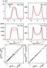 |
Fig. 1 Comparison of the line intensity ratios based on three estimators: |
This is illustrated in Fig. 1, where the models considered correspond to the physical parameters TK = 800 K, n(H2) = 2 × 107 cm-3 and χ(o-H2O) = 10-6. The collisional partner is p-H2, and the results being compared are obtained using the QCT CRC of Faure et al. (2007) and STS quantum CRC of Dubernet et al. (2009) (respectively labelled QCT and quant. in the following). These CRC sets are more extensively discussed in Sect. 3. The two bottom panels show the variation in  (left panel) and max(Ij)quant./max(Ij)QCT (right panel) as a function of
  . Considering the integrated intensity, it can be seen that most of the Wj and ratios show maximum differences of the order of 25%. The two dashed lines in the left panel correspond to straight lines of slopes 0.75 and 1.25, so they delimit a maximum deviation of 25%. Considering the peak intensity (right panel), it can be seen that the correlation between the max(Ij) and ratios is better than for the case of the integrated intensity. In that case, the maximum differences are lower than 10%. The dashed lines correspond to straight lines of slopes 0.9 and 1.1. The four upper panels illustrate that the three estimators start to lead to different ratios when the line profiles of the two models differ. In this figure, we report the brightness temperature for the impact parameter that crosses the centre of the sphere. The profile obtained with the p–H2 QCT CRC corresponds to the black curves. The red curves correspond to the profiles obtained with the p–H2 quantum CRC, and scaled by the ratio
  ,
,  , and max(Ij)QCT/max(Ij)quant.. In other words, the red curves would correspond to line profiles that would lead to a ratio of unity, when compared to the black curve and depending on the estimator used. It can be seen that for the 330–321 line, since the line profiles derived from the two CRC sets are identical, the ratio obtained from the three estimators are identical, too. On the other hand, for example for the 312–221 line, the three estimators lead to different ratios since the line profiles obtained using the two CRC sets differ.
Finally, we emphasise that, in principle, any of the three estimators could be used in order to perform the comparisons presented in the next sections. The conclusions would not be affected by this choice thanks to the good correlation between the ratios obtained with those three estimators. We prefer to use because of its simplicity and because it reduces the line intensity simply to two parameters, the averaged excitation temperature and the line opacity, the first quantity being a useful indicator of how far the line is from thermalization.
2.2. Comparison of rate coefficient sets
To compare two CRC sets, noted SET1 and SET2, we consider the values taken by the ratios  , where
  is defined by Eq. (1) and where the index j stands for the jth radiative transition. The comparisons are made considering the statistics on the M radiative lines that respect the criteria:
-
the line does not show substantial population inversion (i.e., we adopt as a selection criterion that the opacity of a line in the inverted region cannot be greater than 0.5% of the opacity of the line in the thermal region.)
the upper level of the line has an energy below the Nth level (labelled as Nmax in what follows)
-
the intensity of the line as given by Eq. (1) is above 10 mK.
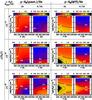
Fig. 2 Comparison of the mean (m) and normalised standard deviations (σ/m, given by Eq. (4)) for the ratios
 (left column) and
  (right column). The intensities are defined by Eq. (1). The statistical analysis is performed on the lines that involve the first Nmax = 20 o–H2O energy levels. The comparison deals with p–H2 CRC. The quantum CRC with p–H2 are from Dubernet et al. (2009) and Daniel et al. (2011), the quantum CRC with He from Green et al. (1993) and the QCT CRC are from Faure et al. (2007). In the case of the quantum CRC, the rates considered are the STS CRC with H2 in j2 = 0. The comparison is performed at the water abundances χ(H2O) = 10-8, 10-6, and 10-4 (rows).
 (4)Additionally, we discuss the results using the normalised standard deviation defined as σ/m rather than σ.
3. Comparison between various H2O CRC
In what follows, we discuss the H2O line intensity predictions based on the three CRC sets that have been widely used, i.e. the quantum H2O – He CRC of Green et al. (1993), the QCT CRC of Faure et al. (2007), and the quantum CRC of Dubernet et al. (2006, 2009) and Daniel et al. (2010, 2011).
3.1. o–H2O QCT and quantum STS CRC with H2 compared to quantum He CRC
In this section, various comparisons are made between the quantum STS CRC calculated with either p–H2 (Dubernet et al. 2009; Daniel et al. 2011) or o–H2 (Daniel et al. 2011), the quantum STS CRC calculated with He (Green et al. 1993), and the QCT calculations (Faure et al. 2007). When referring to the quantum H2 STS CRC, it is assumed that the CRC stands for the CRC where H2 remains in its fundamental rotational energy level (i.e. either j2 = 0 for p–H2 or j2 = 1 for o–H2 with j2 being the H2 rotational quantum number). We note that QCT rate coefficients are not STS, but were obtained for thermal populations of p–H2 and o–H2; i.e., they are thermalised CRC (see below). In the RT calculations, the CRC calculated with He are scaled according to the differing reduced masses of the H2O–He and H2O–H2 systems to emulate collisions with H2.
3.1.1. p–H2 rate coefficients
A first comparison is made between the o–H2O / p–H2 CRC sets obtained with the quantum calculations and the QCT calculations, both with respect to the quantum calculations performed with He. The mean and normalised standard deviations of the ratios  are represented in Fig. 2 for various water abundances and by considering the o–H2O lines with upper energy levels below the 20th level (Eu < 900 K). It appears that the behaviour of the xj ratios can be distinguished between two regimes, which are separated by a threshold (noted n in what follows) in the water volume density n(H2O) = n(H2) × χ(H2O). For water volume densities n(H2) × χ(H2O) > n, the mean value is around 1 and the normalised standard deviation takes low values (typically below 0.1). This corresponds to the thermalised regime where the line intensity ratios are basically independent of the adopted CRC set. In this regime, most of the lines show large optical depths. These depths imply that the critical densities of the lines become lower than in the optically thin limit4, hence producing the thermalization of the level populations. For n(H2) χ(H2O) < n, the level populations are determined by both collisional and radiative processes, making the mean value differ from one and leading to an increase in the normalised standard deviation. In what follows, this regime is referred as subthermal regime.
In Fig. 2 we show a comparison of the line intensity ratios obtained with the quantum p–H2 CRC (left column) and QCT p–H2 CRC (right column), both compared to the quantum He CRC. Examining the p–H2 CRC, we see that independently of the abundance considered, the mean value is in the range 0.45 < m < 1.35. The normalised standard deviation is below 0.5 for all the free parameter space, which means that most of the lines (roughly 70% of the lines considered) show deviations of less than 50% around the mean value. In other words, the main effect introduced by considering the H2 CRC will be to scale the line intensities with respect to the intensities derived from the He CRC. The maximum difference in the scaling factor is encountered at high temperature and low H2 volume densities, where the line intensities based on the H2 CRC are found to be lower by a factor around ~2, for χ(H2O) = 10-8. Additionally, the relative line intensities are expected to vary from one set to the other, with maximum variations of the order of 50% for the bulk of the lines.
The QCT calculations show slightly larger differences, as expected since they correspond to thermalised CRC. Indeed, we find that irrespective of the water vapour abundance, the mean value of the ratios is in the range 1 < m < 2.9, for the whole parameter space considered here. The normalised standard deviation can take values of up to ~0.7. The spread of the ratio around the mean value is of the same order as the one found for the quantum p-H2 CRC.
In Fig. 4 (right column), we show a direct comparison of the results predicted by the STS and QCT CRC. Independently of the water abundance, the QCT CRC predict higher intensities (a factor 2 higher) than the STS CRC. This is because the QCT calculations are a thermal average over the H2 energy levels and because of the large differences of the CRC for H2 in its fundamental state j2 = 0 and in the j2 = 2 state. This is discussed further when considering the thermalised CRC (see Sect. 3.2).
3.1.2. o–H2 rate coefficients
A second comparison concerns the results obtained with o–H2 as a collisional partner. The results obtained with the quantum and QCT CRC are compared to the results obtained with He in Fig. 3. Qualitatively, the H2 quantum and QCT calculations compares closely to the results obtained with He. The main effect concerns the overall scaling of the ratios. In the subthermal regime, the intensity ratios obtained using o–H2 are higher than the one obtained using He, irrespective of the water abundance. A typical increase of 50% is found for the intensity of the lines, with mean values that can be higher than three in the regime of low temperatures and low densities. This result is expected from a direct consideration of CRC obtained with o–H2. Indeed, these rates are typically higher than the rates with He, by factors of up to a factor 10, so the water energy levels are more easily populated when considering o–H2 as a collisional partner. This results in brighter lines. Additionally, we note that the normalised standard deviation is high, and its variations are correlated with the variations in the mean value; i.e, the higher the mean value, the higher the normalised standard deviation.
A direct comparison of the results obtained with the quantum and QCT calculations is shown in Fig. 4 for o–H2 (left column). The differences found for the intensities are modest as long as the water abundance is such that χ(H2O) ≥ 10-6. In that case, the mean value is found to be around one, and the normalised standard deviation is below 0.3 for all the parameter space. The main differences are found for n(H2) < 107 cm-3 and χ(H2O) ~ 10-8 cm-3 where mean values in the range 1.5 < m < 2 are obtained.
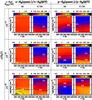 |
Fig. 4 Comparison of the results based on the quantum CRC from Dubernet et al. (2009) and Daniel et al. (2011) with the QCT CRC from Faure et al. (2007), for both o–H2 (left column) and p–H2 (right column). |
3.2. Quantum thermalised CRC with QCT or STS CRC
In this section, we compare the intensities predicted using the quantum STS CRC with the one derived using the thermalised CRC (both defined in Dubernet et al. 2009; Daniel et al. 2011), defined as  (5)In this expression,
  stands for the STS CRC from state i to state j for the H2O molecule, and it corresponds to the transition
  for the H2 molecule. These thermalised CRC thus consider the possibility of energy transfer for both the target molecule (H2O in the present case) and the collider. The populations of the H2 energy levels (noted n(j2) in the above expression) are assumed to be in thermal equilibrium, so that the populations are given by the Boltzmann distribution. In principle, any astrophysical study should consider thermalised rather than STS CRC when dealing with line excitation. In practice, the H2O molecule (and its isotopomers in Faure et al. 2012) is the only molecule for which thermalised CRC have been calculated with a quantum approach. In what follows, we emphasise the effects introduced by considering thermalised rather than STS CRC, keeping in mind that the current findings obtained for the case of water vapour can be extrapolated to other molecules.
The thermalised CRC differ from the quantum STS CRC in two ways. In the following discussion, we consider the case of the collisions with p–H2. At low temperature (i.e. TK ≤ 50 K), only the fundamental level of the p–H2 molecule is substantially populated. The thermalised CRC thus reduce to Rij ~ Cij(0 → 0) + Cij(0 → 2). At low temperature, the second term of this expression is often negligible compared to the first term, except for the H2O transitions for which the variation in the energy induced by the collision is higher than the energy needed to excite the p–H2 molecule to its first excited state. In the case of p–H2, this corresponds to transitions that satisfy ΔEij > 500 K. For these transitions, the term Cij(0 → 2) starts to be dominant in the evaluation of the thermalised CRC since such a rate can be higher by up to a factor 10 in comparison to the STS CRC where H2 remains at its fundamental level. The main effect induced by this process is to efficiently populate the H2O energy levels for the levels with energies higher than 500 K. This is illustrated in Fig. 5, for a model with parameters n(H2) = 106 cm-3, TK = 50 K, and χ(H2O) = 10-4. In this figure, we report the water vapour-level populations averaged over radius. It can be seen that for the levels with energies below 500 K, the STS and thermalised CRC give similar results for the level populations. On the other hand, for the levels with energies higher than 500 K, the populations obtained using the thermalised CRC are generally ten times higher than the one obtained from the STS CRC. In the case of low temperatures, these differences are irrelevant for any astrophysical study since the levels higher than 500 K correspond to transitions that are far below the detection limit of the current telescopes. This example is, however, given to emphasise the effect introduced by the terms Cij(0 → 2), the same effect being found at higher temperatures. However, at higher temperatures, the transitions from the j2 = 2 state make the influence of those terms less evident when considering the level populations, as discussed below.
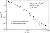 |
Fig. 5 Populations of the o–H2O energy levels as a function of the level energy, for a model with parameters n(H2) = 106 cm-3, TK = 50 K, and χ(H2O) = 10-4. The populations obtained with the state-to-state CRC correspond to the open boxes, whereas the one obtained with the thermalised CRC correspond to the filled boxes. |
At higher temperature, the first p–H2 excited state starts to be substantially populated. Collisions from the state j2 = 2 thus influence the evaluation of the thermalised CRC. In this case, all the H2O transitions are affected by the scaling of the CRC due to the term n(j2 = 2) × Cij(2 → 2). In the case of the H2O molecule, the term Cij(2 → 2) is generally larger than Cij(0 → 0) by a factor that ranges from two to ten depending on the transition. Consequently, the thermalised CRC for all the transitions are increased overall since at the temperatures of 100,200,500 K, the population of the j2 = 2 state accounts for 3, 28, and 58% of the total p–H2 molecules, respectively. As an example, at 200 K, all the thermalised CRC are increased by factors in the range 1.5–3.5 depending on the transition. Additionally, as discussed in the case of the low temperatures, the CRC for the transitions with Δij > 500 K will be increased due to the term Cij(0 → 2).
Finally, Fig. 6 shows a comparison of the results based on thermalised and STS CRC, for temperatures in the range 20 − 100 K and for the first ten o–H2O rotational energy levels. From this figure, it appears that the temperature at which the thermalised CRC start to influence the line intensities is around TK ~ 60 K.
3.2.1. Comparison of the thermalised, STS, and QCT CRC
In Fig. 7, we compare the quantum STS (Dubernet et al. 2009; Daniel et al. 2011) and QCT (Faure et al. 2007) CRC with the results obtained with the thermalised CRC for p–H2 (Dubernet et al. 2009; Daniel et al. 2011). It can be seen that adopting the thermalised CRC strongly influences the results. Indeed, in the limit of low density (i.e. n(H2) < 107 cm-3), both STS and QCT CRC give results that can differ by more than a factor 3, if we consider the mean value. Such high differences are found over all the temperatures considered here for what concerns the STS CRC. On the other hand, the differences between the QCT and thermalised CRC decrease with temperature. Above 400 K, the mean value obtained from the comparison of the QCT and thermalised CRC is below two.
In Fig. 8, we compare the results based on thermalised and STS (Daniel et al. 2011) CRC for the o–H2 symmetry. In this figure, we see that the thermalised CRC give similar results as the STS CRC, with a mean value in the range 1 < m < 1.2 and normalised standard deviation below 0.15 for all the parameter space. The results are shown for a water abundance χ(H2O) = 10-8, but the results are similar for other abundances. The similarity of the derived line intensities is because the terms that involve the j2 = 1 state or j2 = 3 state are similar in magnitude.
Figure 9 show the  ratios for both o–H2 and p–H2, for eight H2O transitions commonly observed with the HIFI and PACS spectrometers onboard Herschel. For each line, the ratios for the prediction based on the o–H2 set are given in the left-hand panel, while the ratios obtained from the CRC that involve p–H2 are given in the right one. We note the similarity of the intensity ratio obtained for both the o–H2 and p–H2 symmetries. This behaviour is discussed further in Sect. 4. The figure corresponds to a water abundance χ(H2O) = 10-8, and it appears that the two CRC sets will lead to qualitatively similar predictions for the line intensities. Indeed, the maximum variations which are found are close to 3, in the worst case. For the lines considered here, and considering collisions with o–H2 (the most abundant symmetry for H2 in hot media), the o–H2O lines that show the largest differences (i.e. greater than a factor of ~2) are the 110 − 101, 221 − 212, 330 − 221 lines. These differences are found at n(H2) < 107 cm-3 for all the temperatures considered here. On the other hand, some lines show only small variations from one set to the other, with intensities that agree within 20% (e.g. 212–101; 303–212; 312–303; 414–303). Moreover, we find that for the majority of the lines, the predictions based on the QCT CRC give lower intensities for the o–H2 symmetry (for all the lines except the 312–303 for which a ratio between 0.6 and 0.8 is found at high temperatures). This implies that an analysis based on the QCT CRC will tend to underestimate the water abundance.
3.2.2. Behaviour of the thermalised CRC
A striking feature when considering the comparison of the STS and thermalised CRC arises from the behaviour at low temperature. Indeed, the greatest differences are found in the range 200 − 400 K between those sets. Simply considering that the population of the p–H2j2 = 2 level increases with temperature, one would expect the differences between those two sets to behave similarly, to reach a maximum when the fundamental level is depopulated. On the contrary, the highest differences are found around 200 K and tend to diminish while the temperature increases. This effect is due to the terms  with Δj2 ≥ 2. In order to quantify the influence of those terms, we used an ad hoc set of CRC. In this set, the thermalised CRC are calculated setting all the CRC with Δj2 ≠ 0 to 0. The comparison between the results based on the STS, QCT, and thermalised CRC with this ad hoc set is shown in Fig. 10. The comparison is made at a density n(H2) = 2 × 107 cm-3 and for a water abundance X(H2O) = 10-8. The choice of these parameters is based on the results shown in Fig. 7, where it can be seen that for both the QCT and STS CRC, these parameters correspond to the maximum differences encountered. Considering the mean value obtained for the ratio
  we see that the mean value has its maximum at 200 K and then decreases with temperature. This proves that the terms with Δj2 ≥ 2 are responsible of the large differences encountered at low temperatures. Considering the mean value for the ratios
  , we find that it has a constant value ~ 1.0 over the whole temperature range. The normalised standard deviation decreases from 0.4 to 0.3 as the temperature increases. In other words, the ad hoc set of CRC and the QCT CRC gives the same results within ~30%. This shows that the main drawback of the QCT approximation is that it does not correctly reproduce the terms Cij(0 → 2). This result is not surprising since these transitions have large rate coefficients when there is a quasi-resonance between the H2O and H2 rotational levels, i.e. transitions with Δij > 500 K. At the QCT level, quasi-resonant effects are not included properly owing to the approximate quantization procedure.
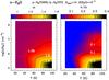 |
Fig. 6 Comparison of the results based on the thermalised and STS CRC from Dubernet et al. (2009) and Daniel et al. (2011) for gas temperatures in the range 20–100 K and for a water abundance χ(H2O) = 10-4. |
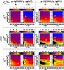 |
Fig. 7 Comparison of the results based on the QCT CRC from Faure et al. (2007) (left column) and state-to-state CRC from Dubernet et al. (2009) and Daniel et al. (2011) (right column), both with the thermalised CRC from Dubernet et al. (2009) and Daniel et al. (2011) for p–H2. |
Critical densities for the lines that involve the first 15 o–H2O energy levels, at TK = 200 K.
3.3. Discussion
In the previous sections, we compared the results of various CRC sets for o–H2O. The comparisons were made by considering the lines that involve energy levels below the 20th one (i.e. Eu < 900 K). With respect to the water symmetry, calculations were also performed for the p–H2O molecule and the conclusions were found to be similar; i.e., the quantum thermalised and QCT CRC give qualitatively similar results for the line intensities, when considering both o–H2 and p–H2 as collisional partners, with maximum differences for the bulk of the lines of about a factor 3.
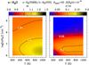 |
Fig. 8 Comparison of the results based on the thermalised and STS CRC from Daniel et al. (2011) for o–H2 and for gas temperatures in the range 200–1000 K and for a water abundance χ(H2O) = 10-8. |
With respect to the number of H2O levels considered, a similar statistical analysis has been performed considering the lines that involve the first 35 energy levels. The differences for the ratios were found to be greater for the lines with Eu > 900 K. This qualitatively results in larger variations in the normalised standard deviations (i.e. would magnify the scale of σ in Figs. 2–4). This is illustrated in Fig. 11 where the mean value and standard deviations are given, for the ratio between the o-H2 STS and QCT CRC. In this figure, we consider all the lines with energy level below the 35th level and for the case of a water abundance of χ(H2O) = 10-6. The results are to be compared to the results shown in Fig. 4 where only the first 20 levels were considered.
Finally, to a first order, it can be seen that the variations in intensities from one set to the other are linearly correlated to the CRC variations. This is illustrated by considering the critical densities related to the various sets of CRC discussed in the previous sections, which are reported in Table 1. Comparing, as an example, the critical densities related to the p–H2 QCT and thermalised CRC, we can see that the maximum differences is a factor 3, which is similar to the maximum difference found for the intensity ratio (see Sect. 3.2).
4. The o–H2 / p–H2 dichotomy
At the present time, apart from H2O, only a few collisional systems have been treated that consider both o–H2 and p–H2 as collisional partners (i.e. CO by Wernli et al. (2006); HC3N by Wernli et al. (2007a); SiS by Lique & Kłos (2008); Kłos & Lique (2008); H2CO by Troscompt et al. (2009); HNC by Dumouchel et al. (2011); CN− by Kłos & Lique (2011); SO2 by Cernicharo et al. (2011); HF by Guillon & Stoecklin (2012); HDO by Faure et al. (2012)). Except in the CN− case, a common conclusion is that the o–H2 CRC are larger than for p–H2. In the particular case of water, the differences are rather large, with CRC for o–H2 that can be larger by up to a factor ten compared to p–H2. This implies that the population of the high-energy levels through collisions with o–H2 will be favoured. At the present time, only few a detailed discussions exist that treats the differences in the excitation of a given molecule and consider the effects introduced by the differing collisional partners. A short discussion of the influence of the H2 OTPR ratio was made by Cernicharo et al. (2009), where a few water-vapour lines were considered for the case of a model describing a protoplanetary disk. This has also been discussed for the H2CO molecule. Troscompt et al. (2009) find that the H2 OTPR was crucial in explaining the excitation of the 110 − 111 line and that it is possible to accurately constrain the H2 OTPR ratio from its observation. On the other hand, Guzmán et al. (2011) find that for the physical conditions which are typical of the Horsehead nebula, the H2CO lines observed in their study are insensitive to the H2 OTPR. A similar conclusion was obtained by Parise et al. (2011) for the deuterated isotopomers of H , which were found to be marginally affected by the H2 OTPR for the conditions typical of prestellar cores (see also Pagani et al. 2009). In what follows, we discuss some characteristics of the water-vapour excitation with respect to collisions with o–H2 or p–H2.
To study the influence of the H2 symmetry, we compared the ratio of the values taken by for the quantum CRC (i.e.  ). In the comparison, we considered both the STS and thermalised CRC. For a given line, we computed the mean value and the normalised standard deviation by summing over all the the models that correspond to the parameter space defined in Sect. 2. We used the same selection for the lines as previously and as are given by the criteria indicated in Sect. 2.
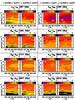 |
Fig. 9 Ratio |
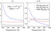 |
Fig. 10 Comparison of the mean (left column) and normalised standard deviation (right column) obtained for the ratios |

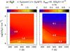 |
Fig. 11 Mean value and normalised standard deviation obtained comparing the quantum CRC from Dubernet et al. (2009) and Daniel et al. (2011) and QCT CRC from Faure et al. (2007), for a water abundance of χ(H2O) = 10-6 cm-3. The lines retained in the comparison have an energy below the one of the 35th level of o–H2O. |
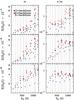 |
Fig. 12 Mean value (left column) and normalised standard deviation (right column) for the |
4.1. State-to-state rate coefficients
The mean value and normalised standard deviation are plotted in Fig. 12, for the three values of the water abundance considered in this work. In this figure, we see that the mean value and normalised standard deviation will depend differently on the collisions with o–H2 or p–H2 according to the energy of the upper level involved in the transition. Additionally, there is a correlation between the sensitivity of the transition to the o–H2/ p–H2 symmetry with the position of the upper energy level on the J-ladder5. Qualitatively, an increase in the energy of the upper level will be accompanied by an increase in both the mean value and normalised standard deviation. For the transitions that involve an upper energy level below 500 K, we find that independently of the water abundance, the mean value is around one and the normalised standard deviation takes low values (below one). Those lines are thus marginally affected by the collisional partner. For the lines with an upper energy level above 500 K, the transitions that are the less affected by the nature of the collisional partner are the transitions where the upper energy level is a backbone level (cf. Fig. 12). For these transitions, the mean value remains relatively low (typically below 2.5) for all the values of the water abundance. The normalised standard deviation is minimal for those transitions, especially when the water abundance is low. This implies that the intensity of these transitions will be only marginally affected by the symmetry of the collisional partner. The transitions that are the most affected are the ones for which the upper level is not a backbone level, while the lower level is backbone level (cf. Fig. 12). These transitions should be good indicators of the H2 OTPR of the gas.
Mean values and normalised standard deviations for the ratios obtained with the thermalised CRC from Dubernet et al. (2009) and Daniel et al. (2011), with parameters in the range 20 < TK < 100 K and 105 < n(H2) < 2 × 108 cm-3.
4.2. Thermalised rate coefficients
In the previous section, on the basis of the quantum STS CRC, it was shown that the H2 OTPR would differentially influence the intensities of the water transitions. In this section, the same analysis is performed using the thermalised quantum CRC, for high gas temperatures (Tk > 200 K) and low gas temperatures (Tk < 100 K).
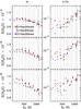 |
Fig. 13 Same as Fig. 12 but considering the quantum thermalized CRC from Dubernet et al. (2009) and Daniel et al. (2011). |
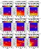 |
Fig. 14 Comparison of the ratio |
4.2.1. High temperature
Figure 13 shows the means and normalised standard deviations for the ratios obtained using the thermalised quantum CRC. From this figure, it appears that the bulk of the lines are mainly insensitive to the H2 OTPR, unlike what was obtained using the STS CRC. For the transitions that involve an upper energy level with energy below 500 K, the mean value is found to be close to one, independently of the water abundance considered. For the transitions that involve higher levels, we find that there is a departure from the mean value of one but the departure is modest, since most of the intensity ratios are in the range 0.7 < m < 1.1. Additionally, the normalised standard deviations are low, i.e. σ/m < 0.3, which means that ~70% of the lines considered in the analysis show variations of less than 30% around the mean value. Interestingly, the transitions that involve energy levels higher than 500 K are generally found brighter when considering the collisions with p–H2 than when considering the collisions with o–H2. This effect is induced by the increase in magnitude of the CRC with ΔEij > 500 K, which was discussed in Sect. 2.
4.2.2. Low temperatures
To discuss the low-temperature regime, we ran models with free parameters in the range TK ∈ [20 K; 100 K], n(H2) ∈ [105; 2 × 10⁸] cm-3 and χ(H2O) ∈ { 10-8;10-6;10-4 } . The mean values and normalised standard deviations are calculated for each line by considering all the models of the grid. In Table 2, we give the mean values and standard deviations for all the lines. From this table, it appears that all the lines that are considered are affected by the H2 OTPR. The main effect, as discussed earlier, is to obtain an increase in intensity when considering o–H2 as a collisional partner for the transitions with upper energy level below 500 K. On the other hand, for the levels with an upper energy level above 500 K, considering p–H2 as a collisional partner results in higher intensities. Additionally, the line intensities are affected differentially by the symmetry of the collisional partner. This differential effect is presented in Fig. 14 where the intensity ratios are shown for some of the lines that involve the lowest energy levels of o–H2O. From this figure it can be seen that under specific physical conditions, the intensity ratio can take high values for certain lines (i.e. larger than 15, like for example for the 221 − 212) while it remains low for other lines (i.e. below 2, like for example for the 414 − 303). Since, the lines depend differentially on the H2 OTPR, it is in principle possible to determine the H2 OTPR for the molecules of the gas from an accurate modelling of the water line intensities observations. In practice, however, this can be a difficult task due to the dependence of the line intensities on other parameters of the model, such as the gas temperature, H2 volume density, and geometry of the source. Moreover, this is only feasible if it relies on a large set of observations. This puts strong limits on the usefulness of water for deriving the H2 OTPR at low temperature (TK < 50 K) since only a few transitions will be observable with reasonable sensitivity (i.e. with RMS < 10 mK).
5. Dust radiative pumping
All the comparisons performed in Sects. 2 and 3 ignored the possibility of pumping by IR and submillimetre dust radiation. This would correspond to an extreme case, not physically relevant to all astrophysical objects. Indeed, as an example, radiative pumping by continuum photons plays an important role in the H2O excitation in AGB circumstellar envelopes. In short, considering this additional mechanism in the population of the water energy levels would reduce the differences between line intensities obtained from differing CRC. This is illustrated in Fig. 15, where we consider the ratios obtained from the STS CRC. In this example, we chose to compare the results based on these CRC since we found in Sect. 4 that the respective intensities show large differences, thereby emphasing the role played by dust radiation. The model parameters are n(H2) = 106 cm-3, TK = 200 K, and χ(H2O) = 10-8. In the model, we assume a gas-to-dust mass ratio of 100, and the dust composition corresponds to a mixture of astrophysical silicates and amorphous carbon grains, with opacities taken from Draine & Lee (1984). In the modelling, we varied the dust temperature (Td) from 5 K to 200 K. Moreover, to compute , we assume Tbg = Td for the background temperature. From this figure, we see that, while the mean values and standard deviations are high at low dust temperatures (m ~ 7 and σ ~ 5), they are considerably reduced when Td increases. For dust temperatures above 50 K, we obtain m ~ 1 and σ < 0.2, which implies that the influence of differing CRC starts to be minimal since the population of the H2O energy levels is dominated by radiative pumping and no longer by the collisions.
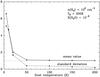 |
Fig. 15 Mean value and standard deviation as a function of the dust temperature. The ratios considered are obtained considering the quantum ortho- and para- STS CRC from Dubernet et al. (2009) and Daniel et al. (2011). |
6. Conclusions
We performed non-local non-LTE excitation and radiative transfer calculations aiming at comparing the line intensities predicted for water vapour when making use of differing CRC sets. The CRC sets compared are the He quantum rate coefficients (Green et al. 1993), H2 quantum rate coefficients of (Dubernet et al. 2006, 2009; Daniel et al. 2010, 2011), and H2 quasi-classical rate coefficients (Faure et al. 2007). The comparison was performed at relatively high temperature (200 K < TK < 1000 K) and an emphasis was made on the comparison of the H2 CRC sets, since the quantum rate coefficients have only lately become available and many recent astrophysical studies have made use of the QCT calculations. In the absence of radiative pumping by dust photons, it was found that the results based on the quantum and QCT rate coefficients sets will lead to line intensities that qualitatively agree, i.e. which are of the same order of magnitude, for the parameter space considered in this work. However, the H2O line emission can differ by a factor of ~ 3, in the regime of low water abundance (χ(H2O) ~ 10-8) and moderate H2 volume densities (n(H2) < 107 cm-3).
These differences should not drastically affect the conclusions obtained from modelling the water excitation in astrophysical objects, but the water vapour abundance derived on the basis of the QCT rate coefficients will differ with the one derived from the quantum rate coefficients, with differences still up to a factor of ~ 3. We note, however, that such differences will be attenuated by the presence of a dust continuum source of radiation. Additionally, masing lines are not considered in the present analysis. A similar comparison for the case of masing lines is presented in Daniel & Cernicharo (2012), where the impact induced by the CRC on the lines that will be observable with ALMA is discussed. Finally, we emphasise that the impact of the various CRC sets is discussed on the basis of statistics over the most intense lines. The current results can thus be affected to some extent by the choice of the subset of lines used in the analysis.
The differences found between the QCT and quantum CRC can give clues to the uncertainty introduced in the modelling owing to the uncertainties on the rate coefficients. Indeed, as discussed in Dubernet et al. (2009) and Daniel et al. (2010), the QCT and quantum CRC typically agree within a factor of 3 for the highest rate coefficients. In the current study, we obtain the same factor between the line intensities obtained with two sets. Therefore, in a first approximation, the error on the rate coefficients will translate similarly to line intensities. Recently, Yang et al. (2011) find a good agreement between experimental integral cross sections and quantum calculations, showing the good accuracy of the PES on which the quantum calculations are based. Depending on the energy of the level considered and the gas temperature, it was said in Dubernet et al. (2009) and Daniel et al. (2010) that the accuracy of the quantum CRC will range from a few to a few ten percentage points and such errors should scale linearly on line intensities.
We performed additional test calculations with an ad hoc set of thermalised CRC in which the STS rate coefficients associated to the H2 transitions with Δj2 ≠ 0 were removed. The comparison of the results obtained with this ad hoc set and the QCT rate coefficients showed particularly good agreement. Over the temperature range T = 200–1000 K, the intensities predicted with those two sets agree within 30%. It is concluded that the main drawback of the QCT approximation is that it does not correctly reproduce the terms Cij(0 → 2).
By considering the quantum STS and quantum thermalised CRC, it was found that line intensities will be largely affected by considering the first excited state, in the case of p–H2. The differences start to be non-negligible (i.e. greater than 20%) for temperatures higher than TK ~ 60 K, reaching a maximum of a factor ~3 around 200 K. On the other hand, the intensities predicted with the STS and thermalised CRC are similar for the collisions that involve o–H2. Such behaviour can be extrapolated to other molecules that show strong differences for the collisions between o–H2 and p–H2. Indeed, these differences arise because of the interaction with the quadrupole of H2, and significant differences for the CRC with p–H2 or o–H2 imply that the STS rate coefficients for p–H2 in j2 = 0 or j2 = 2 will show large differences, too. Therefore, the use of STS rather than thermalised CRC for such molecules will lead to overestimating of the molecular abundances for temperatures higher than TK ~ 60 K.
By comparing the line intensities obtained using either o–H2 or p–H2 as a collisional partner, we found that under particular physical conditions (n(H2) and TK), the water lines will be differentially affected by the symmetry of the H2 molecule. This effect is obtained when the gas temperature is low, i.e. TK < 100 K. In contrast, at high temperature, the lines become insensitive to the H2 symmetry. Since some transitions will show large intensity variations with respect to the H2 symmetry, the modelling of the water excitation may provide a means to derive the H2 OTPR. The lines to be considered in such an estimate will, however, depend on the physical conditions prevailing in the object under study, so it is necessary to perform a case-by-case modelling.
I.e. nc = Aul⟨β⟩/Cul where β is the probability that a photon escapes the medium; with β = 1 in the optically thin case and β ~ 1/τ when the line becomes optically thick.
As a reminder, H2O is an asymmetric top with quantum numbers denoted as either J,Ka,Kc or J,K + ,K − . A backbone level corresponds to the lower level in energy for a given value of the principal quantum number J. This level corresponds to the lowest possible value for the difference Ka − Kc.
Acknowledgments
The authors want to thank the anonymous referee, whose detailed comments enabled them to improve the content of the current article. This paper was partially supported within the programme CONSOLIDER INGENIO 2010, under grant “Molecular Astrophysics: The Herschel and ALMA Era.- ASTROMOL” (Ref.: CSD2009-00038). We also thank the Spanish MICINN for funding support through grants AYA2006-14876 and AYA2009-07304. J.R.G. is supported by a Ramón y Cajal research contract from the Spanish MICINN and co-financed by the European Social Fund.
References
- Cernicharo, J., & Crovisier, J. 2005, Space Sci. Rev., 119, 29 [NASA ADS] [CrossRef] [Google Scholar]
- Cernicharo, J., Thum, C., Hein, H., et al. 1990, A&A, 231, L15 [NASA ADS] [Google Scholar]
- Cernicharo, J., Gonzalez-Alfonso, E., Alcolea, J., Bachiller, R., & John, D. 1994, ApJ, 432, L59 [NASA ADS] [CrossRef] [Google Scholar]
- Cernicharo, J., González-Alfonso, E., & Bachiller, R. 1996, A&A, 305 [Google Scholar]
- Cernicharo, J., Pardo, E., Serabyn, E., et al. 1999, ApJ, 520, L131 [NASA ADS] [CrossRef] [Google Scholar]
- Cernicharo, J., Goicoechea, J. R., Daniel, F., et al. 2006a, ApJ, 649, L33 [NASA ADS] [CrossRef] [Google Scholar]
- Cernicharo, J., Goicoechea, J. R., Pardo, J. R., & Asensio-Ramos, A. 2006b, ApJ, 642, 940 [NASA ADS] [CrossRef] [Google Scholar]
- Cernicharo, J., Ceccarelli, C., Ménard, F., Pinte, C., & Fuente, A. 2009, ApJ, 703, L123 [NASA ADS] [CrossRef] [Google Scholar]
- Cernicharo, J., Spielfiedel, A., Balança, C., et al. 2011, A&A, 531, A103 [NASA ADS] [CrossRef] [EDP Sciences] [Google Scholar]
- Cheung, A. C., Rank, D. M., Townes, C. H., Thornton, D. D., & Welch, W. J. 1969, Nature, 221, 626 [NASA ADS] [CrossRef] [Google Scholar]
- Daniel, F., & Cernicharo, J. 2008, A&A, 488, 1237 [NASA ADS] [CrossRef] [EDP Sciences] [Google Scholar]
- Daniel, F., & Cernicharo, J. 2012, A&A, submitted [Google Scholar]
- Daniel, F., Dubernet, M.-L., Pacaud, F., & Grosjean, A. 2010, A&A, 517, A13 [NASA ADS] [CrossRef] [EDP Sciences] [Google Scholar]
- Daniel, F., Dubernet, M.-L., & Grosjean, A. 2011, A&A, 536, A76 [NASA ADS] [CrossRef] [EDP Sciences] [Google Scholar]
- Draine, B. T., & Lee, H. M. 1984, ApJ, 285, 89 [Google Scholar]
- Dubernet, M.-L., & Grosjean, A. 2002, A&A, 390, 793 [NASA ADS] [CrossRef] [EDP Sciences] [Google Scholar]
- Dubernet, M.-L., Daniel, F., Grosjean, A., et al. 2006, A&A, 460, 323 [NASA ADS] [CrossRef] [EDP Sciences] [Google Scholar]
- Dubernet, M.-L., Daniel, F., Grosjean, A., & Lin, C. Y. 2009, A&A, 497, 911 [NASA ADS] [CrossRef] [EDP Sciences] [Google Scholar]
- Dumouchel, F., Kłos, J., & Lique, F. 2011, Phys. Chem. Chem. Phys., 13, 8204 [NASA ADS] [CrossRef] [Google Scholar]
- Faure, A., & Josselin, E. 2008, A&A, 492, 257 [NASA ADS] [CrossRef] [EDP Sciences] [Google Scholar]
- Faure, A., Valiron, P., Wernli, M., et al. 2005, J. Chem. Phys., 122, 221102 [NASA ADS] [CrossRef] [PubMed] [Google Scholar]
- Faure, A., Crimier, N., Ceccarelli, C., et al. 2007, A&A, 472, 1029 [NASA ADS] [CrossRef] [EDP Sciences] [Google Scholar]
- Faure, A., Wiesenfeld, L., Scribano, Y., & Ceccarelli, C. 2012, MNRAS, 420, 699 [NASA ADS] [CrossRef] [MathSciNet] [Google Scholar]
- Goicoechea, J. R., Rodriguez-Fernandez, N. J., & Cernicharo, J. 2004, ApJ, 600, 214 [NASA ADS] [CrossRef] [Google Scholar]
- Goicoechea, J. R., Cernicharo, J., Karska, A., et al. 2012, A&A, in press, DOI: 10.1051/0004-6361/201219912 [Google Scholar]
- González-Alfonso, E., Cernicharo, J., Bachiller, R., & Fuente, A. 1995, A&A, 293, L9 [NASA ADS] [Google Scholar]
- González-Alfonso, E., Cernicharo, J., Alcolea, J., & Orlandi, M. A. 1998, A&A, 334, 1016 [NASA ADS] [Google Scholar]
- Gonzalez-Alfonso, E., Smith, H. A., Fischer, J., & Cernicharo, J. 2004, ApJ, 613, 247 [NASA ADS] [CrossRef] [Google Scholar]
- Grosjean, A., Dubernet, M.-L., & Ceccarelli, C. 2003, A&A, 408, 1197 [NASA ADS] [CrossRef] [EDP Sciences] [Google Scholar]
- Green, S., Maluendes, S., & McLean, A. D. 1993, ApJS, 85, 181 [NASA ADS] [CrossRef] [Google Scholar]
- Guillon, G., & Stoecklin, T. 2012, MNRAS, 420, 579 [NASA ADS] [CrossRef] [Google Scholar]
- Guzmán, V., Pety, J., Goicoechea, J. R., Gerin, M., & Roueff, E. 2011, A&A, 534, A49 [NASA ADS] [CrossRef] [EDP Sciences] [Google Scholar]
- Herczeg, G. J., Karska, A., Bruderer, S., et al. 2012, A&A, 540, A84 [NASA ADS] [CrossRef] [EDP Sciences] [Google Scholar]
- Hogerheijde, M. R., Bergin, E. A., Brinch, C., et al. 2011, Science, 334, 338 [NASA ADS] [CrossRef] [PubMed] [Google Scholar]
- Kessler, M. F., Steinz, J. A., Anderegg, M. E., et al. 1996, A&A, 315, L27 [NASA ADS] [Google Scholar]
- Kłos, J., & Lique, F. 2008, MNRAS, 390, 239 [NASA ADS] [CrossRef] [Google Scholar]
- Kłos, J., & Lique, F. 2011, MNRAS, 418, 271 [NASA ADS] [CrossRef] [Google Scholar]
- Kristensen, L. E., van Dishoeck, E. F., Bergin, E. A., et al. 2012, A&A, 542, A8 [NASA ADS] [CrossRef] [EDP Sciences] [Google Scholar]
- Lique, F., & Kłos, J. 2008, J. Chem. Phys., 128, 034306 [NASA ADS] [CrossRef] [Google Scholar]
- Lis, D. C., Phillips, T. G., Goldsmith, P. F., et al. 2010, A&A, 521, L26 [NASA ADS] [CrossRef] [EDP Sciences] [Google Scholar]
- Melnick, G. J., Stauffer, J. R., Ashby, M. L. N., et al. 2000, ApJ, 539, L77 [NASA ADS] [CrossRef] [Google Scholar]
- Menten, K., & Melnick, G. J. 1991, ApJ, 377, 647 [NASA ADS] [CrossRef] [Google Scholar]
- Menten, K. M., Melnick, G. J., Phillips, T. G., & Neufeld, D. A. 1990a, ApJ, 363, L27 [NASA ADS] [CrossRef] [Google Scholar]
- Menten, K. M., Melnick, G. J., & Phillips, T. G. 1990b, ApJ, 350, L41 [NASA ADS] [CrossRef] [Google Scholar]
- Neufeld, D. A., & Kaufman, M. J. 1993, ApJ, 418, 263 [NASA ADS] [CrossRef] [Google Scholar]
- Neufeld, D. A., Lepp, S., & Melnick, G. J. 1995, ApJ, 100, 132 [Google Scholar]
- Neufeld, D. A., Gonzalez-Alfonso, E., Melnick, G. J., et al. 2011, ApJ, 727, L29 [NASA ADS] [CrossRef] [Google Scholar]
- Nordh, H. L., von Schéele, F., Frisk, U., et al. 2003, A&A, 402, L21 [NASA ADS] [CrossRef] [EDP Sciences] [Google Scholar]
- Pagani, L., Vastel, C., Hugo, E., et al. 2009, A&A, 494, 623 [NASA ADS] [CrossRef] [EDP Sciences] [Google Scholar]
- Parise, B., Belloche, A., Du, F., Güsten, R., & Menten, K. M. 2011, A&A, 526, A3 [NASA ADS] [CrossRef] [EDP Sciences] [Google Scholar]
- Phillips, T. G., Kwan, J., & Huggins, P. J. 1980, in IAU Symp. 87, ed. B. H. Andrew (Dordrecht: Reidel), 21 [Google Scholar]
- Phillips, T. R., Maluendes, S., McLean, A. D., & Green, S. 1994, J. Chem. Phys., 101, 5824 [NASA ADS] [CrossRef] [Google Scholar]
- Phillips, T. R., Maluendes, S., & Green, S. 1996, ApJS, 107, 467 [NASA ADS] [CrossRef] [Google Scholar]
- Pilbratt, G. L., Riedinger, J. R., Passvogel, T., et al. 2010, A&A, 518, L1 [CrossRef] [EDP Sciences] [Google Scholar]
- Rothman, L. S., Gordon, I. E., Barbe, A., et al. 2009, J. Quant. Spec. Radiat. Transf., 110, 533 [Google Scholar]
- Royer, P., Decin, L., Wesson, R., Barlow, M. J., et al. 2010, A&A, 518, L145 [NASA ADS] [CrossRef] [EDP Sciences] [Google Scholar]
- Troscompt, N., Faure, A., Wiesenfeld, L., Ceccarelli, C., & Valiron, P. 2009, A&A, 493, 687 [NASA ADS] [CrossRef] [EDP Sciences] [Google Scholar]
- Troscompt, N., Faure, A., Maret, S., et al. 2009, A&A, 506, 1243 [NASA ADS] [CrossRef] [EDP Sciences] [Google Scholar]
- Valiron, P., Wernli, M., Faure, A., et al. 2008, J. Chem. Phys., 129, 134306 [NASA ADS] [CrossRef] [PubMed] [Google Scholar]
- van Dishoeck, E. F. 2004, ARA&A, 42, 119 [NASA ADS] [CrossRef] [Google Scholar]
- van Dishoeck, E. F., Kristensen, L. E., Benz, A. O., et al. 2011, PASP, 123, 138 [NASA ADS] [CrossRef] [Google Scholar]
- Waters, J. W., Kakar, R. K., Kuiper, T. B. H., et al. 1980, ApJ, 235, 57 [NASA ADS] [CrossRef] [Google Scholar]
- Watson, D. M., Bohac, C. J., Hull, C., et al. 2007, Nature, 448, 1026 [NASA ADS] [CrossRef] [PubMed] [Google Scholar]
- Wernli, M., Valiron, P., Faure, A., et al. 2006, A&A, 446, 367 [NASA ADS] [CrossRef] [EDP Sciences] [Google Scholar]
- Wernli, M., Wiesenfeld, L., Faure, A., & Valiron, P. 2007a, A&A, 464, 1147 [NASA ADS] [CrossRef] [EDP Sciences] [Google Scholar]
- Wernli, M., Wiesenfeld, L., Faure, A., & Valiron, P. 2007b, A&A, 475, 391 [NASA ADS] [CrossRef] [EDP Sciences] [Google Scholar]
- Yang, C.-H., Sarma, G., Parker, D. H., Ter Meulen, J. J., & Wiesenfeld, L. 2011, J. Chem. Phys., 134, 204308 [NASA ADS] [CrossRef] [Google Scholar]
All Tables
Critical densities for the lines that involve the first 15 o–H2O energy levels, at TK = 200 K.
Mean values and normalised standard deviations for the ratios obtained with the thermalised CRC from Dubernet et al. (2009) and Daniel et al. (2011), with parameters in the range 20 < TK < 100 K and 105 < n(H2) < 2 × 108 cm-3.
All Figures
|
Fig. 1 Comparison of the line intensity ratios based on three estimators: |
| In the text | |
|
Fig. 2 Comparison of the mean (m) and normalised standard deviations (σ/m, given by Eq. (4)) for the ratios |
| In the text | |
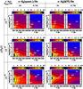 |
Fig. 3 Same as Fig. 2 but for the collisions that involve o–H2. |
| In the text | |
|
Fig. 4 Comparison of the results based on the quantum CRC from Dubernet et al. (2009) and Daniel et al. (2011) with the QCT CRC from Faure et al. (2007), for both o–H2 (left column) and p–H2 (right column). |
| In the text | |
|
Fig. 5 Populations of the o–H2O energy levels as a function of the level energy, for a model with parameters n(H2) = 106 cm-3, TK = 50 K, and χ(H2O) = 10-4. The populations obtained with the state-to-state CRC correspond to the open boxes, whereas the one obtained with the thermalised CRC correspond to the filled boxes. |
| In the text | |
|
Fig. 6 Comparison of the results based on the thermalised and STS CRC from Dubernet et al. (2009) and Daniel et al. (2011) for gas temperatures in the range 20–100 K and for a water abundance χ(H2O) = 10-4. |
| In the text | |
|
Fig. 7 Comparison of the results based on the QCT CRC from Faure et al. (2007) (left column) and state-to-state CRC from Dubernet et al. (2009) and Daniel et al. (2011) (right column), both with the thermalised CRC from Dubernet et al. (2009) and Daniel et al. (2011) for p–H2. |
| In the text | |
|
Fig. 8 Comparison of the results based on the thermalised and STS CRC from Daniel et al. (2011) for o–H2 and for gas temperatures in the range 200–1000 K and for a water abundance χ(H2O) = 10-8. |
| In the text | |
|
Fig. 9 Ratio |
| In the text | |
|
Fig. 10 Comparison of the mean (left column) and normalised standard deviation (right column) obtained for the ratios |
| In the text | |
|
Fig. 11 Mean value and normalised standard deviation obtained comparing the quantum CRC from Dubernet et al. (2009) and Daniel et al. (2011) and QCT CRC from Faure et al. (2007), for a water abundance of χ(H2O) = 10-6 cm-3. The lines retained in the comparison have an energy below the one of the 35th level of o–H2O. |
| In the text | |
|
Fig. 12 Mean value (left column) and normalised standard deviation (right column) for the |
| In the text | |
|
Fig. 13 Same as Fig. 12 but considering the quantum thermalized CRC from Dubernet et al. (2009) and Daniel et al. (2011). |
| In the text | |
|
Fig. 14 Comparison of the ratio |
| In the text | |
|
Fig. 15 Mean value and standard deviation as a function of the dust temperature. The ratios considered are obtained considering the quantum ortho- and para- STS CRC from Dubernet et al. (2009) and Daniel et al. (2011). |
| In the text | |
Current usage metrics show cumulative count of Article Views (full-text article views including HTML views, PDF and ePub downloads, according to the available data) and Abstracts Views on Vision4Press platform.
Data correspond to usage on the plateform after 2015. The current usage metrics is available 48-96 hours after online publication and is updated daily on week days.
Initial download of the metrics may take a while.