| Issue |
A&A
Volume 546, October 2012
|
|
|---|---|---|
| Article Number | A82 | |
| Number of page(s) | 9 | |
| Section | The Sun | |
| DOI | https://doi.org/10.1051/0004-6361/201220111 | |
| Published online | 09 October 2012 | |
Damped kink oscillations of flowing prominence threads
1
Centre for Mathematical Plasma Astrophysics, Department of
Mathematics, KU Leuven,
Celestijnenlaan 200B,
3001
Leuven,
Belgium
e-mail: This email address is being protected from spambots. You need JavaScript enabled to view it.
2
Solar Physics and Space Plasma Research Centre
(SP 2RC), University of Sheffield,
Hicks Building, Hounsfield
Road, Sheffield
S3 7RH,
UK
Received:
26
July
2012
Accepted:
14
September
2012
Abstract
Transverse oscillations of thin threads in solar prominences are frequently reported in high-resolution observations. Two typical features of the observations are that the oscillations are damped in time and that simultaneous mass flows along the threads are detected. Flows cause the dense threads to move along the prominence magnetic structure while the threads are oscillating. The oscillations have been interpreted in terms of standing magnetohydrodynamic (MHD) kink waves of the magnetic flux tubes, which support the threads. The damping is most likely due to resonant absorption caused by plasma inhomogeneity. The technique of seismology uses the observations combined with MHD wave theory to estimate prominence physical parameters. This paper presents a theoretical study of the joint effect of flow and resonant absorption on the amplitude of standing kink waves in prominence threads. We find that flow and resonant absorption can either be competing effects on the amplitude or both can contribute to damp the oscillations depending on the instantaneous position of the thread within the prominence magnetic structure. The amplitude profile deviates from the classic exponential profile of resonantly damped kink waves in static flux tubes. Flow also introduces a progressive shift of the oscillation period compared to the static case, although this effect is in general of minor importance. We test the robustness of seismological estimates by using synthetic data aiming to mimic real observations. The effect of the thread flow can significantly affect the estimation of the transverse inhomogeneity length scale. The presence of random background noise adds uncertainty to this estimation. Caution needs to be paid to the seismological estimates that do not take the influence of flow into account.
Key words: Sun: filaments, prominences / Sun: oscillations / Sun: corona / magnetohydrodynamics (MHD) / waves
© ESO, 2012
1. Introduction
Solar prominences and filaments are large-scale magnetic structures of the solar corona (see the recent reviews by Labrosse et al. 2010; Mackay et al. 2010, about the physics, dynamics, and modeling of prominences). High-resolution Hα observations reveal that prominences are formed by a myriad of fine structures usually called threads (see, e.g., Lin 2011). Threads are thin and long plasma condensations which outline the prominence magnetic field. Theoretically, prominence threads have been modeled as magnetic flux tubes anchored in the solar photosphere (e.g., Ballester & Priest 1989; Rempel et al. 1999), which are only partially filled with the cool (~104 K) prominence material, i.e., the thread itself, while the rest of the tube is occupied by hot coronal plasma and therefore invisible in Hα images.
Threads are highly dynamic. For example, transverse thread oscillations and propagating waves along the threads are frequently observed in prominences, which have been interpreted in terms of magnetohydrodynamic (MHD) kink waves (see the reviews by Arregui & Ballester 2010; Arregui et al. 2012a). The reported periods are usually in between 2 and 10 min, and the oscillations are typically damped after a few periods (Ning et al. 2009). Resonant absorption, caused by plasma inhomogeneity in the transverse direction to the magnetic field has been proposed as the damping mechanism (e.g., Arregui et al. 2008, 2011; Soler et al. 2009, 2010). In addition, flows and mass motions in prominences have been also reported (e.g., Zirker et al. 1998; Lin et al. 2003; Okamoto et al. 2007). The mean flow velocities are in most cases less than 30 km s-1, although values up to 40–50 km s-1 have been observed in active region prominences. The presence of flow can have a direct impact on the behavior of the waves (see a discussion on this issue in Carbonell et al. 2009). The combined use of both observations and MHD wave theory allows to apply the technique of seismology to solar prominences (see Oliver 2009; Arregui et al. 2012b).
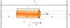 |
Fig. 1 Sketch of the prominence thread model used in this work. |
Some observations point out the simultaneous presence of transverse oscillations and mass flows in prominence threads. The work by Okamoto et al. (2007) is probably the best example. Okamoto et al. (2007) observed an active region prominence with Hinode/SOT using Ca II H-line images. They detected that some threads in the prominence were flowing presumably along the magnetic field with an apparent velocity on the plane of sky of around 40 km s-1. Simultaneously, the threads were oscillating in the transverse direction. The mean period of the oscillations was 3 min. The oscillations were in phase along the whole length of the threads, which was roughly between 3000 km and 16 000 km. Thus, a standing wave interpretation was proposed and the actual wavelength was estimated to be at least 250 000 km, which would correspond to twice the total length of magnetic field lines, approximately.
The observations by Okamoto et al. (2007) motivated a number of theoretical works that aim to interpret the observed thread dynamics. Terradas et al. (2008) interpreted the observations by Okamoto et al. (2007) in terms of standing MHD kink modes and used the observed periods to perform a seismological estimation of a lower bound of the prominence Alfvén speed. Subsequently, Soler & Goossens (2011) revisited the same event and performed both an analytical and a numerical investigation of the influence of flow on the period and amplitude of the standing waves. However, neither Terradas et al. (2008) nor Soler & Goossens (2011) took the damping of the oscillations into account. Okamoto et al. (2007) did not study the evolution in time of the amplitude of the transverse thread oscillations, but damping has been reported in other events (see, e.g., Ning et al. 2009). The main purpose of the present work is therefore to determine the joint effect of flow and resonant absorption on the amplitude of standing kink MHD modes in prominence threads. The resonant damping of kink waves in the presence of flow has been studied in the past in the context of coronal loops (see, e.g., Goossens et al. 1992; Terradas et al. 2010; Soler et al. 2011), but not in the case of prominences.
We apply the general analytic theory developed by Ruderman (2011a,b) for standing kink waves in magnetic flux tubes with a time-dependent background. Analytic expressions for the kink mode amplitude and period as functions of the model parameters are derived. In addition, since the efficiency of resonant damping is directly controlled by the transverse inhomogeneity length scale of the threads, part of the present paper is also devoted to test the impact of flow on the estimation of this parameter using the technique of seismology (Goossens et al. 2008).
This paper is organized as follows. Section 2 contains a description of the prominence thread model used in this work. The mathematical method is presented in Sect. 3, where the main equations are obtained. Then, the impact of the different model parameters on the amplitude of kink modes is studied in Sect. 4. Later, the implications of our results for prominence seismology are discussed in Sect. 5. Finally, the conclusions of this work are given in Sect. 6.
2. Model
The prominence thread model used in this paper is schematically shown in Fig. 1. It is composed of a straight and cylindrical magnetic flux tube of radius R and length L. The z-axis is chosen so that it coincides with the axis of the tube. The magnetic field is B = Bêz, with B constant everywhere. The tube ends are located at z = ± L/2 and are fixed by two rigid walls representing the solar photosphere. The magnetic tube is partially filled with prominence plasma, i.e., the prominence thread, with length Lp and density ρp, while the rest of the tube, i.e., the evacuated part, is occupied by less dense plasma of density ρe. The external plasma represents the coronal medium with density ρc. According to the observed typical values of thread widths and lengths from the high-resolution observations of prominences (see, e.g., Lin 2011), the ranges of realistic values of R and Lp are 50 km ≲ R ≲ 300 km and 3000 km ≲ Lp ≲ 28 000 km. The total tube length, L, is very difficult to measure from the observations, but one can relate L to the typical spatial scale in prominences and filaments, i.e., L ~ 105 km. These estimations of L, Lp, and R imply that prominence threads are very thin and long structures. The ratio of the prominence density to the coronal density is a large parameter. The value ρp/ρc = 200 is usually considered in the literature, although we do not fix the density contrast at the present stage. For simplicity we assume that the evacuated part of the tube has the same density as the corona so that we take ρe = ρc.
In addition, in the prominence thread we consider a transversely inhomogeneous transitional layer of thickness l, that continuously connects the internal prominence density, ρp, to the external coronal density, ρc. The limits l/R = 0 and l/R = 2 correspond to a thread without transverse transitional layer and a fully inhomogeneous thread in the radial direction, respectively. The present paper adopts the β = 0 approximation, where β refers to the ratio of the gas pressure to the magnetic pressure. Hence, the plasma temperature is irrelevant for this study and we can choose the density profile in the transitional layer arbitrarily. The presence of this transitional layer introduces damping of the kink waves by resonant absorption (see, e.g., Goossens et al. 1992, 2006, 2011). Finally, as a key ingredient of the model, there is a flow along the tube with a constant velocity u0. As a consequence, the prominence thread moves along the tube as a block at the velocity u0.
Standing kink waves supported by the present model have been investigated in the past under several simplifications. In the absence of flow and for l/R = 0, there are the studies by Joarder et al. (1997) and Díaz et al. (2001) in Cartesian geometry, and by Díaz et al. (2002) in cylindrical geometry. These works considered arbitrary values of R and L, which involves a complicated mathematical formalism. Dymova & Ruderman (2005) derived a more simplified approach valid for thin cylindrical tubes, i.e., R/L ≪ 1. The thin tube approximation provides very accurate results when compared to the general solution. Subsequently, the case l/R ≠ 0 in the absence of flow was addressed by Dymova & Ruderman (2006) and Soler et al. (2010) again in the thin tube approximation, and by Arregui et al. (2011) in the general case. In the presence of flow, the problem was studied by Terradas et al. (2008) numerically and by Soler & Goossens (2011) combining analytic and numerical methods. However, both works considered l/R = 0 and so resonant damping was absent from their investigations.
3. Mathematical method
The mathematical method followed in this work is based on the theory developed by Ruderman (2011a,b), who derived the governing equation describing standing kink waves in the thin tube and thin boundary approximations (see Eq. (23) of Ruderman 2011b). We refer the reader to the original paper by Ruderman (2011b) for a detailed derivation of the governing equation. The thin tube approximation means that we are restricted to the case R/L ≪ 1 and R/Lp ≪ 1. This is not a problem since the realistic values of L, Lp, and R satisfy these constraints. The thin boundary approximation means that we take l/R ≪ 1, i.e., an abrupt but continuous transition in density in the transverse direction.
Equation (23) of Ruderman (2011b) can be solved
analytically using the Wentzel-Kramers-Brillouin (WKB) approximation (see, e.g., Bender & Orszag 1978). The WKB approximation is
appropriate when the background properties are slowly varying functions of space and/or
time. In the present application of the WKB approximation we assume that the timescale
related to the waves, e.g., the period, is much shorter than the timescale related to the
changes of the background configuration. As in Soler
& Goossens (2011) we define the parameter δ as
 (1)with
u0 the flow velocity and L the total length
of the tube. The validity of the WKB approximation is restricted to small values of
δ so that Pδ ≪ 1, where P is the period
of the standing kink wave. In the observations by Okamoto
et al. (2007), the mean flow velocity and period are
u0 ≈ 40 km s-1 and P ≈ 3 min. For
L ~ 105 km these values give Pδ ≈ 0.072.
Hence the condition of applicability of the WKB approximation is fulfilled in the present
case. Using the WKB approximation, Ruderman (2011b)
arrives at the expression for the transverse displacement of the fundamental mode of the
magnetic tube, η(t,z), namely
(1)with
u0 the flow velocity and L the total length
of the tube. The validity of the WKB approximation is restricted to small values of
δ so that Pδ ≪ 1, where P is the period
of the standing kink wave. In the observations by Okamoto
et al. (2007), the mean flow velocity and period are
u0 ≈ 40 km s-1 and P ≈ 3 min. For
L ~ 105 km these values give Pδ ≈ 0.072.
Hence the condition of applicability of the WKB approximation is fulfilled in the present
case. Using the WKB approximation, Ruderman (2011b)
arrives at the expression for the transverse displacement of the fundamental mode of the
magnetic tube, η(t,z), namely
![Mathematical equation: \begin{equation} \eta (t,z) = A(t) W_0(t,z) \exp \left[ {\rm i} F(t,z) \right] \exp \left[ {\rm i} \int_0^t \omega(\tau) {\rm d}\tau\right], \end{equation}](/articles/aa/full_html/2012/10/aa20111-12/aa20111-12-eq40.png) (2)where
A(t),
W0(t,z), and
F(t,z) are real functions, and
ω(t) is the instantaneous frequency at time
t. The function A(t) is positive and
represents the oscillation amplitude as a function of time. The function
F(t,z) represents a small phase shift that can be
neglected (see Ruderman 2011b) and, therefore, it is
omitted hereafter. The function W0(t,z)
satisfies the equation
(2)where
A(t),
W0(t,z), and
F(t,z) are real functions, and
ω(t) is the instantaneous frequency at time
t. The function A(t) is positive and
represents the oscillation amplitude as a function of time. The function
F(t,z) represents a small phase shift that can be
neglected (see Ruderman 2011b) and, therefore, it is
omitted hereafter. The function W0(t,z)
satisfies the equation 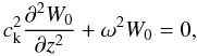 (3)along with the boundary
conditions
W0(t, ± L/2) = 0
due to photospheric line-tying. The function
W0(t,z) is defined so that
W0(t,z) > 0 and
max[W0(t,z)] = 1. In Eq. (3) ck is the kink
velocity, which in our model is defined as
(3)along with the boundary
conditions
W0(t, ± L/2) = 0
due to photospheric line-tying. The function
W0(t,z) is defined so that
W0(t,z) > 0 and
max[W0(t,z)] = 1. In Eq. (3) ck is the kink
velocity, which in our model is defined as 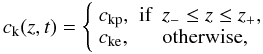 (4)where
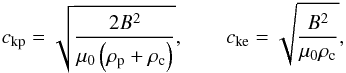 (5)with
μ0 the magnetic permeability of free space and
(5)with
μ0 the magnetic permeability of free space and
 (6)with
z0 corresponding to the position of the center of the
prominence thread with respect to the center of the magnetic tube at t = 0.
Note that z0 < 0 if the thread is
initially located on the left-hand side to the center of the tube, whereas
z0 > 0 if the thread is initially
located on the right-hand side. We also note that the flow velocity,
u0, only explicitly appears in the expressions of
z + and z−.
(6)with
z0 corresponding to the position of the center of the
prominence thread with respect to the center of the magnetic tube at t = 0.
Note that z0 < 0 if the thread is
initially located on the left-hand side to the center of the tube, whereas
z0 > 0 if the thread is initially
located on the right-hand side. We also note that the flow velocity,
u0, only explicitly appears in the expressions of
z + and z−.
The equation governing the amplitude A(t) corresponds to
Eq. (66) of Ruderman (2011b), namely  (7)where
 ![Mathematical equation: \begin{eqnarray} \label{eq:i} I &=& \int_{-L/2}^{L/2} \left( \rho_{\rm i} + \rc \right) W_0^2 \der z, \\[1mm] \Gamma &=& \frac{\pi}{2} \frac{\mu}{B^2} \frac{\omega^4}{R} \sum_{n=1}^N \int_{-L/2}^{L/2} \left( \rho_{\rm i} - \rc \right) W_0 w_n(r_n) \der z \nonumber \\[1mm] \label{eq:gamma} & & \times \int_{-L/2}^{L/2} \frac{ \rho_{\rm t}(r_n) - \rc}{\left| \Delta_n \right|} W_0 w_n(r_n) \der z. \end{eqnarray}](/articles/aa/full_html/2012/10/aa20111-12/aa20111-12-eq64.png) In
the expressions of I and Γ, ρi is the internal
density given by
In
the expressions of I and Γ, ρi is the internal
density given by  (10)and
ρt(r) is the density in the transitional
layer, with ρt(rn)
the corresponding value at the nth resonant position
r = rn. The function
wn is the eigenfunction of the Alfvén
boundary value problem
(10)and
ρt(r) is the density in the transitional
layer, with ρt(rn)
the corresponding value at the nth resonant position
r = rn. The function
wn is the eigenfunction of the Alfvén
boundary value problem  (11)along with
wn(r) = 0 at
z = ± L/2, where
(11)along with
wn(r) = 0 at
z = ± L/2, where
 is the local Alfvén velocity
squared. In Eq. (11)
ωA,n(r) is the
nth Alfvén eigenvalue. The eigenfunction
wn satisfies the normalization condition
is the local Alfvén velocity
squared. In Eq. (11)
ωA,n(r) is the
nth Alfvén eigenvalue. The eigenfunction
wn satisfies the normalization condition
 (12)where
δmn is the Kronecker delta. The position of
the nth resonance, rn, is
given by the condition
(12)where
δmn is the Kronecker delta. The position of
the nth resonance, rn, is
given by the condition  . Finally, the quantity
Δn is given by
. Finally, the quantity
Δn is given by
 (13)We consider the case
l/R = 0 in order to compare with the
expressions used by Soler & Goossens (2011).
In the absence of resonant damping Γ = 0 and the equation for the amplitude
A(t) (Eq. (7)) can be expanded to
(13)We consider the case
l/R = 0 in order to compare with the
expressions used by Soler & Goossens (2011).
In the absence of resonant damping Γ = 0 and the equation for the amplitude
A(t) (Eq. (7)) can be expanded to  (14)We compare Eq. (14) to Eq. (20) of Soler & Goossens (2011). The only difference between the equation
for the amplitude used by Soler & Goossens
(2011) and the equation derived using the more general method by Ruderman (2011b) resides in the term with the temporal
derivative of I in Eq. (14). The equation of Soler & Goossens
(2011) does not take the dependence of I on time into account. For
the fundamental mode and slow flows, I may be roughly independent on time.
This can be checked once W0(t,z) is found. In
that case, the equation of Soler & Goossens
(2011) is an approximate description of the fundamental mode amplitude.
(14)We compare Eq. (14) to Eq. (20) of Soler & Goossens (2011). The only difference between the equation
for the amplitude used by Soler & Goossens
(2011) and the equation derived using the more general method by Ruderman (2011b) resides in the term with the temporal
derivative of I in Eq. (14). The equation of Soler & Goossens
(2011) does not take the dependence of I on time into account. For
the fundamental mode and slow flows, I may be roughly independent on time.
This can be checked once W0(t,z) is found. In
that case, the equation of Soler & Goossens
(2011) is an approximate description of the fundamental mode amplitude.
Using the method developed by Ruderman (2011a,b) and summarized in the previous paragraphs, the problem of studying damped standing oscillations of flowing threads is reduced to finding the functions W0(t,z) and A(t), along with the expression for the instantaneous frequency ω(t). This is done in the following subsections.
3.1. Finding W0(t,z) and ω(t)
To find the function W0(t,z) we need to
solve the boundary value problem defined in Eq. (3) with
W0(t, ± L/2) = 0.
In addition, since the equilibrium is piecewise constant in z we need to
provide additional boundary conditions at
z = z±. Since
z = z± correspond to contact
discontinuities, the boundary conditions are that
W0(t,z) is continuous at
z = z± (Goedbloed & Poedts 2004). Thus, the process here is equivalent to the
process followed by Soler & Goossens (2011)
to find their function Q1(t,z). The reader is
referred to Soler & Goossens (2011) for
details. The expression for W0(t,z) is
![Mathematical equation: \begin{equation} W_0(t,z) = \left\{ \begin{array}{lll} D_1 \sin \left[ \frac{\omega}{\vke} \left( z + \frac{L}{2} \right) \right] &\textrm{if}& z < z_-, \\ \cos \left( \frac{\omega}{\vkp} z + \phi \right) &\textrm{if}& z_- \leq z \leq z_+, \\ D_2 \sin \left[ \frac{\omega}{\vke} \left( z - \frac{L}{2} \right) \right] &\textrm{if}& z > z_+, \end{array} \right. \label{eq:expw0} \end{equation}](/articles/aa/full_html/2012/10/aa20111-12/aa20111-12-eq92.png) (15)where
φ = φ(t) is a time-dependent phase,
and D1 and D2 are given by
(15)where
φ = φ(t) is a time-dependent phase,
and D1 and D2 are given by
![Mathematical equation: \begin{equation} D_1 = \frac{\cos \left( \frac{\omega}{\vkp} z_- + \phi \right)}{\sin \left[ \frac{\omega}{\vke} \left( z_- + \frac{L}{2} \right) \right]}, \qquad D_2 = \frac{\cos \left( \frac{\omega}{\vkp} z_+ + \phi \right)}{\sin \left[ \frac{\omega}{\vke} \left( z_+ - \frac{L}{2} \right) \right]}\cdot \end{equation}](/articles/aa/full_html/2012/10/aa20111-12/aa20111-12-eq96.png) (16)The expression for
W0(t,z) takes the condition
max[W0(t,z)] = 1 into account.
(16)The expression for
W0(t,z) takes the condition
max[W0(t,z)] = 1 into account.
The time-dependent frequency, ω(t), requires to obtain
first the time-dependent dispersion relation by providing additional boundary conditions
which enable us to eliminate the time-dependent phase, φ. These
additional conditions are that
∂W0/∂z
is continuous at z = z±. The expression
for φ is ![Mathematical equation: \begin{equation} \phi = - \frac{\omega}{\vkp} z_- - \arctan \left\{ \frac{\vkp}{\vke} \cot \left[\frac{\omega}{\vke}\left( z_- + \frac{L}{2} \right) \right] \right\}, \end{equation}](/articles/aa/full_html/2012/10/aa20111-12/aa20111-12-eq99.png) (17)and the dispersion
relation is Eq. (14) of Soler & Goossens
(2011). The fundamental mode corresponds to the solution with the lowest
frequency. By performing the first-order expansion of their Eq. (14) with respect to the
small parameter
ρc/ρp, Soler & Goossens (2011) obtained an approximate
expression for ω(t) (their Eq. (15)), which in the limit
ρc/ρp ≪ 1
realistic of prominences reduces to
(17)and the dispersion
relation is Eq. (14) of Soler & Goossens
(2011). The fundamental mode corresponds to the solution with the lowest
frequency. By performing the first-order expansion of their Eq. (14) with respect to the
small parameter
ρc/ρp, Soler & Goossens (2011) obtained an approximate
expression for ω(t) (their Eq. (15)), which in the limit
ρc/ρp ≪ 1
realistic of prominences reduces to  (18)This is the expression
for
(18)This is the expression
for  used in the following computations. In the absence of flow,
u0 = 0 and ω becomes independent of time and
corresponds to the normal mode frequency (see Soler et al.
2010).
used in the following computations. In the absence of flow,
u0 = 0 and ω becomes independent of time and
corresponds to the normal mode frequency (see Soler et al.
2010).
Since W0(t,z) is known, we can compute the
integral I (Eq. (8)). The
result is ![Mathematical equation: \begin{eqnarray} \label{eq:icomp} I &=& 2 \rc D_1^2 \left[ \frac{z_- + L/2}{2} - \frac{\vke}{4 \omega} \sin \left( \frac{2 \omega}{\vke} (z_- + L/2) \right) \right] \nonumber \\ &\quad -& 2 \rc D_2^2 \left[ \frac{z_+ - L/2}{2} - \frac{\vke}{4 \omega} \sin \left( \frac{2 \omega}{\vke} (z_+ - L/2) \right) \right] \nonumber \\ &\quad +& (\rp+\rc) \left\{ \frac{z_+ - z_-}{2} + \frac{\vkp}{4 \omega} \left[ \sin\left( \frac{2 \omega}{\vkp}z_+ + \phi \right) \right. \right. \nonumber \\ &\quad-& \left. \left. \sin\left( \frac{2 \omega}{\vkp}z_- + \phi \right) \right] \right\}. \end{eqnarray}](/articles/aa/full_html/2012/10/aa20111-12/aa20111-12-eq106.png) (19)As
before, we take advantage of the fact that the fundamental mode is the solution with the
lowest frequency. We perform the first-order expansion of Eq. (19) with respect to the small parameter
ρc/ρp to get
the approximate expression of I valid for the fundamental mode, namely
(19)As
before, we take advantage of the fact that the fundamental mode is the solution with the
lowest frequency. We perform the first-order expansion of Eq. (19) with respect to the small parameter
ρc/ρp to get
the approximate expression of I valid for the fundamental mode, namely
 (20)Thus, we find
that the integral I is time-independent in this approximation. We can now
check the equation for the amplitude used by Soler
& Goossens (2011) in the absence of resonant damping, i.e.,
l/R = 0. When I is
constant in time, Eq. (14) reverts to
Eq. (20) of Soler & Goossens (2011).
Therefore, the equation for the amplitude used by Soler
& Goossens (2011) is justified in this approximation.
(20)Thus, we find
that the integral I is time-independent in this approximation. We can now
check the equation for the amplitude used by Soler
& Goossens (2011) in the absence of resonant damping, i.e.,
l/R = 0. When I is
constant in time, Eq. (14) reverts to
Eq. (20) of Soler & Goossens (2011).
Therefore, the equation for the amplitude used by Soler
& Goossens (2011) is justified in this approximation.
With the use of the approximate expression for I given in Eq. (20), we obtain the general equation for the
amplitude when l/R ≠ 0 (Eq. (7)), namely  (21)The next step is to
compute Γ in order to integrate Eq. (21).
(21)The next step is to
compute Γ in order to integrate Eq. (21).
3.2. Finding Γ
Equation (9) for Γ takes the possibility
of multiple resonances into account. From hereon we assume that there is only one
resonance position at r = r1, and we set
N = 1 in Eq. (9). This
is the same assumption as in Ruderman (2011b,
Sect. 5.1). This assumption was also used by Soler et al. (2010) and was later checked to be correct by Arregui et al. (2011). In addition, we take into account that the
density in the evacuated part of the tube, ρe, is set equal to
the coronal density, ρc, so that
l/R = 0 in the evacuated region.
Thus, we can change the limits of integration in Eq. (9) from
[− L/2,L/2]
to
[z−,z + ] .
Also, since ρp, ρc, and
ρt(r1) are constants, we can
move them out of the integrals. The same is true for |Δ1| since this quantity
is independent of z. Finally, the expression for Γ becomes  (22)with
  (23)At the resonance position
r = r1, so
(23)At the resonance position
r = r1, so
 . By comparing Eqs. (3) and (11) we see that W0 and
wn(r1) are
the eigenfunctions of the same eigenvalue problem when
. By comparing Eqs. (3) and (11) we see that W0 and
wn(r1) are
the eigenfunctions of the same eigenvalue problem when  (24)So, we can put
wn(r1)
proportional to W0, namely
wn(r1) = QW0,
where Q is a constant of proportionality, and Eq. (23) becomes
(24)So, we can put
wn(r1)
proportional to W0, namely
wn(r1) = QW0,
where Q is a constant of proportionality, and Eq. (23) becomes ![Mathematical equation: \begin{eqnarray} \Lambda = Q \int_{z_-}^{z_+} W_0^2 \der z &=& Q \left\{ \frac{z_+ - z_-}{2} + \frac{\vkp}{2 \omega} \left[ \sin \left( \frac{2\omega}{\vkp}z_+ + 2\phi \right) \right. \right. \nonumber \\ \label{eq:lamdba2} &\quad -& \left. \left. \sin \left( \frac{2\omega}{\vkp}z_- + 2\phi \right) \right] \right\}\cdot \end{eqnarray}](/articles/aa/full_html/2012/10/aa20111-12/aa20111-12-eq125.png) (25)As
before, we only take the fundamental mode into account and perform the first-order
expansion of Eq. (25) with respect
to ρc/ρp. We
also use the normalization condition (Eq. (12)) with m = n = 1 to find that
(25)As
before, we only take the fundamental mode into account and perform the first-order
expansion of Eq. (25) with respect
to ρc/ρp. We
also use the normalization condition (Eq. (12)) with m = n = 1 to find that
 in this approximation for the fundamental mode. Thus, we obtain the approximate Λ as
 (26)Now we compute
|Δ1|. To do so we use again the resonant condition
and Eq. (24) to write
(26)Now we compute
|Δ1|. To do so we use again the resonant condition
and Eq. (24) to write
 (27)Hence the
expression for |Δ1| is
(27)Hence the
expression for |Δ1| is  (28)We next write
 (29)where F
is a factor that depends on the form of the transverse density profile. For example,
F = 4/π2 for a linear
profile and F = 2/π for a sinusoidal
profile with r1 = R. The expression
for |Δ1| becomes
(29)where F
is a factor that depends on the form of the transverse density profile. For example,
F = 4/π2 for a linear
profile and F = 2/π for a sinusoidal
profile with r1 = R. The expression
for |Δ1| becomes  (30)Finally, we substitute
all these results in Eq. (22) and arrive
at the expression for Γ, namely
(30)Finally, we substitute
all these results in Eq. (22) and arrive
at the expression for Γ, namely  (31)
(31)
3.3. Time-dependent amplitude A(t)
We substitute Eq. (31) in Eq. (21) to write the equation for the
time-dependent amplitude A(t) as  (32)with
 (33)Equation (32) can be easily integrated using the
expression for ω(t) given in Eq. (18). The result is
(33)Equation (32) can be easily integrated using the
expression for ω(t) given in Eq. (18). The result is ![Mathematical equation: \begin{equation} A(t) = A_0 \left[ \frac{\left( L - \lp \right) \left( L + \frac{1}{3} \lp \right) - 4 \left( z_0 + u_0 t \right)^2}{\left( L - \lp \right) \left( L + \frac{1}{3} \lp \right) - 4 z_0^2} \right]^{1/4} {\rm e}^{ - \gamma \Omega(t)},\label{eq:amp4} \end{equation}](/articles/aa/full_html/2012/10/aa20111-12/aa20111-12-eq141.png) (34)with the function
Ω(t) given by
(34)with the function
Ω(t) given by ![Mathematical equation: \begin{eqnarray} \Omega(t) &=& \frac{\vkp}{u_0} \sqrt{\frac{L}{\lp}} \left[ \arctan\left( \frac{2(z_0+u_0 t)}{\sqrt{ \left( L - \lp \right) \left( L + \frac{1}{3} \lp \right) - 4 \left( z_0 + u_0 t \right)^2 }} \right) \right. \nonumber \\ & -& \left. \arctan\left( \frac{2z_0}{\sqrt{ \left( L - \lp \right) \left( L + \frac{1}{3} \lp \right) - 4 z_0^2 }} \right) \right]\cdot \end{eqnarray}](/articles/aa/full_html/2012/10/aa20111-12/aa20111-12-eq143.png) (35)The
first factor on the right-hand side of Eq. (34), i.e., A0, represents the initial amplitude at
t = 0. The second factor on the right-hand side of Eq. (34), i.e., that with the square brackets, is
the same as that found in Eq. (22) of Soler &
Goossens (2011). This term accounts for the change of the amplitude due to the
motion of the prominence thread along the magnetic tube. This contribution can cause
either amplification or damping depending on the instantaneous position of the thread with
respect to the center of the magnetic tube. This term is equal to unity in the static
case, i.e., for u0 = 0. The third factor on the right-hand
side of Eq. (34) is an exponential factor
that accounts for damping due to resonant absorption.
(35)The
first factor on the right-hand side of Eq. (34), i.e., A0, represents the initial amplitude at
t = 0. The second factor on the right-hand side of Eq. (34), i.e., that with the square brackets, is
the same as that found in Eq. (22) of Soler &
Goossens (2011). This term accounts for the change of the amplitude due to the
motion of the prominence thread along the magnetic tube. This contribution can cause
either amplification or damping depending on the instantaneous position of the thread with
respect to the center of the magnetic tube. This term is equal to unity in the static
case, i.e., for u0 = 0. The third factor on the right-hand
side of Eq. (34) is an exponential factor
that accounts for damping due to resonant absorption.
To recover the result in the static case without flow, we evaluate the limit of
Ω(t) when u0 → 0, namely
 (36)where
ω0 the frequency given in Eq. (18) with u0 = 0. In that case, the
exponential factor on the right-hand side of Eq. (34) becomes
exp(− γω0t), so that we
consistently revert to the static case studied by Soler
et al. (2010) and Arregui et al. (2011).
(36)where
ω0 the frequency given in Eq. (18) with u0 = 0. In that case, the
exponential factor on the right-hand side of Eq. (34) becomes
exp(− γω0t), so that we
consistently revert to the static case studied by Soler
et al. (2010) and Arregui et al. (2011).
4. Parametric study
Here we explore the impact of the various model parameters on the amplitude. In particular we focus on the effects of the thickness of the transitional layer, l/R, and the flow velocity, u0. We assume a linear variation for the density in the transitional layer.
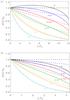 |
Fig. 2 A(t)/A0 as a function of t/P0, with P0 the instantaneous period at t = 0. The numbers next to the various lines indicate the value of l/R used. The solid line is the complete result, while the dashed line is the equivalent result but with u0 = 0. We have used a) z0/L = −0.25 and b) z0/L = 0.1. In all computations Lp/L = 0.1, u0/cAp = 0.1, and ρp/ρc = 200. |
Figure 2 shows A(t)/A0 as a function of t/P0, with P0 = 2π/ω0 the instantaneous period at t = 0. We plot the results for several values of l/R and z0/L, and compare the amplitude obtained in the presence and in the absence of flow. We find that the amplitude in the presence of flow is substantially different from that for u0 = 0 when the transitional layer is very thin, so that damping due to resonant absorption is very weak. In this case the variation of the amplitude is mainly governed by the effect of the flow, described by the factor with the square brackets on the right-hand side of Eq. (34). It is possible to obtain amplification of the amplitude at short times when z0/L < 0 and the transitional layer is very thin (top lines in Fig. 2a). As l/R increases, the damping term, which is the exponential factor on the right-hand side of Eq. (34), becomes more important and the amplitude is almost the same in both cases u0 = 0 and u0 ≠ 0, i.e., the effect of the flow is then of minor importance. When z0/L > 0 (Fig. 2b) amplification is not possible regardless the value of l/R and damping is always observed.
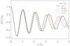 |
Fig. 3 Prominence thread transverse displacement, η(t)/η0, as a function of t/P0, with P0 the instantaneous period at t = 0, for various values of u0/cAp indicated within the figure. In all computations Lp/L = 0.1, l/R = 0.1, z0/L = −0.25, and ρp/ρc = 200. |
Figure 3 displays the thread displacement as a function of t/P0 for different values of the flow velocity (the remaining parameters are indicated in the caption of the figure). We obtain a progressive phase shift between the solutions corresponding to different velocities. This is so because the instantaneous period, P(t) = 2π/ω(t), is a function of the flow velocity according to Eq. (18). However, for the set of parameters used in Fig. 3 the amplitude is weakly affected by the flow velocity. In particular, the value l/R = 0.1 used in Fig. 3 is large enough for the amplitude to be dominated by resonant damping.
5. Implications for prominence seismology
The results presented in this paper have implications for seismology of solar prominences
(see Arregui et al. 2012b). Adopting resonant
absorption as damping mechanism, the inversion technique of Goossens et al. (2008) has been applied to the case of prominence thread
oscillations (see Arregui & Ballester 2010;
Soler et al. 2010). Due to the high density
contrast of the prominence plasma with respect to the coronal plasma, a direct estimation of
l/R is possible when measures of both
period and damping time are available. The value of
l/R inferred by seismology may be
used to test thread models, because the transverse inhomogeneity length scale is a crucial
parameter for the energy balance of the prominence threads with the surrounding hot coronal
plasma (see, e.g., Pojoga 1994; Cirigliano et al. 2004; Labrosse et al.
2010). The analytic equation used to infer
l/R is (Goossens et al. 2008)  (37)where P
and τD are the (constant) period and the damping time obtained
after fitting to the observed oscillation a harmonic function with amplitude proportional to
exp( − t/τD).
This expression does not take the flow of the prominence thread into account. In this
section we test the robustness of seismological estimates when flow is present and
Eq. (37) is used in combination with
typical fitting methods for the oscillation amplitude. In addition, the influence of
background noise is also studied.
(37)where P
and τD are the (constant) period and the damping time obtained
after fitting to the observed oscillation a harmonic function with amplitude proportional to
exp( − t/τD).
This expression does not take the flow of the prominence thread into account. In this
section we test the robustness of seismological estimates when flow is present and
Eq. (37) is used in combination with
typical fitting methods for the oscillation amplitude. In addition, the influence of
background noise is also studied.
5.1. Example
We synthetically generate a signal aiming to represent a prominence thread transverse
oscillation detected with a real instrument. We use the following set of parameters:
Lp/L = 0.1,
l/R = 0.1,
z0/L = −0.05,
ρp/ρc = 200,
and
u0/cAp = 0.1. A
linear density profile in the transitional layer is used. The corresponding theoretical
transverse displacement is displayed in Fig. 4a with
a dashed line. The time series corresponds roughly to 6 oscillation periods. This is
approximately the number of periods observed in time series of real events (see, e.g.,
Ning et al. 2009). To represent the limited
cadence of the instrument we perform a temporal sampling of this signal using,
approximately, 33 points per period. For a typical period of 3 min, this corresponds to a
cadence of about 5 s. This cadence is of the same order as that used in recent
observations (see, e.g., Lin et al. 2009). Later,
we add to the sampled signal a randomly generated noise. In this way we try to account for
the contribution of the background to the total signal and/or to consider unspecified
instrumental uncertainties. Noise is generated with the IDL function randomu. Here, we specify the amplitude of the
background noise as percentage of the signal amplitude at t = 0, namely
 (38)where
ηnoise is the noise amplitude and
η0 is the signal amplitude at t = 0. It is
more frequent in observational astrophysics to use the signal-to-noise ratio, S/N, which
is defined as the power ratio between the signal and the background noise. Assuming that
the power is proportional to the square of the amplitude, the relation between
(38)where
ηnoise is the noise amplitude and
η0 is the signal amplitude at t = 0. It is
more frequent in observational astrophysics to use the signal-to-noise ratio, S/N, which
is defined as the power ratio between the signal and the background noise. Assuming that
the power is proportional to the square of the amplitude, the relation between
 and
S/N is
and
S/N is
 (39)For example,
 corresponds to
S/N = 100. In the present example
we use
corresponds to
S/N = 100. In the present example
we use  , which is equivalent to
S/N = 4. Finally, a smoothing
algorithm is applied to the noisy data. The resulting signal is plotted in Fig. 4a with the solid line. Since the added noise is randomly
generated, we can obtain different synthetic signals depending on the seed used in the
random number generator. The synthetic data displayed in Fig. 4a is the one used in this particular example.
, which is equivalent to
S/N = 4. Finally, a smoothing
algorithm is applied to the noisy data. The resulting signal is plotted in Fig. 4a with the solid line. Since the added noise is randomly
generated, we can obtain different synthetic signals depending on the seed used in the
random number generator. The synthetic data displayed in Fig. 4a is the one used in this particular example.
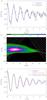 |
Fig. 4 a) Original (dashed) and synthetic (solid) data used in the seismological test. b) Wavelet power spectrum for the dimensionless period, P/P0, corresponding to the synthetic signal displayed in panel a). The white solid line is the original data instantaneous period, whereas the horizontal dotted line is the period obtained from the fitting method. The red solid line denotes 99% of confidence level. c) Comparison of the original (dashed) and fitted signals with noise (solid) and without noise (dotted). |
Figure 4b shows a wavelet power spectrum (Torrence & Compo 1998) of the synthetic signal displayed in Fig. 4a. For comparison we overplot the instantaneous period of the original data. We see that the wavelet spectrum recovers well the period of the original data. However, since the effect of the flow on the period is not very strong and the duration of the time series is limited to 6 periods, the variation of the period with time is not evident in the wavelet spectrum. The added noise also makes difficult the analysis near the end of the time series when the amplitude is low. Based on this result, we believe that the effect of the flow on the period would probably go unnoticed for an observer using wavelet analysis.
We turn again to the synthetic signal of Fig. 4a and
try a different approach. We fit to the synthetic data a typical exponentially damped
harmonic function as  (40)where
a1, a2,
a3, and a4 are four parameters
to fit. The fitted period, P, and damping time,
τD, are
(40)where
a1, a2,
a3, and a4 are four parameters
to fit. The fitted period, P, and damping time,
τD, are
 (41)The fit is made using the
IDL function curvefit. We perform a
fit to the sampled data before and after adding random noise. The result of both fits is
shown in Fig. 4c, where we also plot the original
curve for comparison. First of all, we obtain a progressive phase shift between the
different curves because the fitted function (Eq. (40)) does not take the variation of the period with time into account.
The constant period obtained from the fit to the noisy data is indicated by the horizontal
dotted line in Fig. 4b. This fitted period agrees
well with the maximum in the wavelet spectrum, but overestimates the actual period at
later times.
(41)The fit is made using the
IDL function curvefit. We perform a
fit to the sampled data before and after adding random noise. The result of both fits is
shown in Fig. 4c, where we also plot the original
curve for comparison. First of all, we obtain a progressive phase shift between the
different curves because the fitted function (Eq. (40)) does not take the variation of the period with time into account.
The constant period obtained from the fit to the noisy data is indicated by the horizontal
dotted line in Fig. 4b. This fitted period agrees
well with the maximum in the wavelet spectrum, but overestimates the actual period at
later times.
More importantly, we also find different damping rates for the three curves. The damping of both fitted functions is stronger than the actual damping. In particular, the fitted curve to the noisy data has the strongest damping, i.e., the lowest amplitude. The difference in the damping of the original curve and that of the sampled signal without noise can be attributed to the effect of the flow, whereas in the sampled signal with noise we have to take the additional influence of noise into account. This has a direct consequence on the seismological estimation of l/R using the fitted P and τD in Eq. (37). In the original data we used l/R = 0.1, while the inferred values are l/R = 0.13 for the sampled signal without noise and l/R = 0.16 for the sampled signal with noise. We have not computed the uncertainty of the fitted parameters and, therefore, we do not know the relative error on the estimation of l/R. However, the results of this example suggest that the presence of both flow and noise adds significant uncertainty to the determination of l/R.
5.2. Statistical study
Now, we perform a statistical study of the influence of flow and noise on the determination of l/R and its uncertainty. The purpose here is to know whether the results obtained in the example of the previous subsection are general or, on the contrary, they are particular to this example only. We use the same parameters as in the previous example but vary the value of the flow velocity and the percentage of maximum background noise.
First we fix
(S/N = 4). We follow the procedure
explained before to generate a set of 104 synthetic noisy signals for various
values of u0. The various synthetic signals are generated
using different initial seeds in the random number generator. As in the example, we fit an
exponentially damped harmonic function (Eq. (40)) to each one of the synthetic signals and infer the value of
l/R using Eq. (37). Subsequently, we perform a histogram with
the full set of 104
estimated l/R for each
particular u0. By visual inspection, we determine that the
histograms follow the Gaussian distribution. Therefore, we fit to the histograms a
Gaussian function of the form  (42)with
b0 the height of the Gaussian, μ the mean
value, and σ the standard deviation. We display in Fig. 5a the histograms and their Gaussian fits corresponding
to three values of the flow velocity. For u0 = 0 the Gaussian
mean value matches the actual l/R. As
the flow velocity increases, the mean value is shifted toward larger
l/R, but the width of the Gaussian
is roughly the same regardless of the flow velocity.
(42)with
b0 the height of the Gaussian, μ the mean
value, and σ the standard deviation. We display in Fig. 5a the histograms and their Gaussian fits corresponding
to three values of the flow velocity. For u0 = 0 the Gaussian
mean value matches the actual l/R. As
the flow velocity increases, the mean value is shifted toward larger
l/R, but the width of the Gaussian
is roughly the same regardless of the flow velocity.
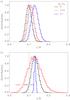 |
Fig. 5 a) Normalized histogram of the seismologically estimated l/R for three values of the flow velocity (indicated within the panel) and a maximum background noise corresponding to 50% of the initial amplitude. b) Same as panel a) but with u0/cAp = 0.1 and three percentages of maximum background noise (indicated next to the lines). In both panels, the dashed lines are the Gaussian fits and the vertical dotted line is the actual l/R. |
On the other hand, Fig. 5b shows equivalent
histograms but for a fixed value of the flow velocity and three
different . We find
that the width of the Gaussian is strongly affected by noise, i.e., the larger the
background noise, the wider the Gaussian. The width of the Gaussian is related to the
uncertainty of l/R. Thus, we
consistently obtain that the uncertainty increases when noise is increased, as expected.
However, the mean value is not affected by the percentage of noise. The effect of noise is
explored in more detail in Fig. 6, which shows the
fitted μ (Fig. 6a)
and σ (Fig. 6b) as a function of
the maximum background noise percentage for three flow velocities. We find
that μ is independent of noise and its shift with respect to the actual
l/R is only determined by the flow
velocity. For the set of parameters used in this test, the mean estimated
l/R when flow is present is larger
than the actual value. On the contrary, the effect of flow on σ is minor
compared to the effect of noise. We obtain that σ is a approximately
linear with the maximum noise percentage.
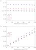 |
Fig. 6 a) Mean value, μ, and b) standard deviation, σ, of the Gaussian distribution of seismologically estimated l/R as functions of the percentage of background noise. The different symbols correspond to different flow velocities (indicated within the panels). The horizontal dotted line in panel a) shows the actual value of l/R. |
Up to here we have obtained that the seismologically
inferred l/R tends to overestimate
the actual value. Our goal now is to determine whether this is the general tendency or
whether this is affected by the choice of the model parameters. There are several
parameters that may affect the estimation of
l/R. In particular, the role of
z0, i.e., the position of the thread with respect to the
center of the magnetic tube at the beginning of the oscillation, is worth being studied.
To do so, we fix
u0/cAp = 0.1,
, and select a particular value
of z0/L (the remaining
parameters are the same as before). For a given
z0/L we repeat the
previously explained procedure to generate the set of synthetic signals and the
corresponding estimations of l/R. We
fit the Gaussian function to the obtained histogram and compute μ and
σ as functions of
z0/L. These results are
displayed in Fig. 7. Regarding μ
(Fig. 7a), we find that the estimated
l/R is larger than the actual value
except when z0/L ≲ −0.1.
When z0 is negative, i.e., the thread is initially located to
the left of the center of the magnetic tube, the effect of flow is to increase the
amplitude until the thread reaches the center of the tube, meaning that flow opposes
resonant damping. This increase of the amplitude compensates the overestimation
of l/R by the fitting method, so
that the mean estimated l/R is closer
to the actual value. On the contrary, when
z0/L ≳ −0.1 the flow
contributes to damping during most of the evolution. This causes an overestimation of
l/R. The behavior
of σ (Fig. 7b) also shows an
increasing trend
with z0/L.
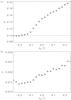 |
Fig. 7 a) Mean value, μ, and b) standard deviation, σ, of the Gaussian distribution of seismologically estimated l/R as functions of z0/L. A maximum background noise of 50% and u0/cAp = 0.1 are used. The horizontal dotted line in panel a) shows the actual value of l/R. |
Based on the results shown in this section, we conclude that flow and noise have two different effects on the estimation of l/R using typical fitting methods in combination with the theoretical inversion formula. An exponentially damped harmonic function has been used as a proxy to the actual oscillation. On the one hand, flow tends to shift the estimated l/R with respect to the actual value. The shift depends specifically on the flow velocity and on the position of the prominence thread at the beginning of the oscillation but, in general, an overestimation of l/R is found in the statistical analysis. On the other hand, as expected, noise adds uncertainty to the estimation. This noise-related uncertainty might be partially reduced if some method able to subtract the background noise is applied to the raw data. However, some uncertainty intrinsically related to the effect of flow might remain even if the influence of noise is completely removed.
Real data are frequently affected by gaps in the time series. This issue has not been taken into account in the present analysis. The consideration of gaps would add more complexity to the analysis and, probably, would result in a new source of error. Appropriate methods accounting for the effect of gaps in the signals should be used (see, e.g., Carbonell et al. 1992). This is worth being investigated in future works.
6. Conclusions
In this paper we have studied the joint effect of resonant absorption and flow on the amplitude of standing kink waves in prominence threads. The present work extends the previous paper by Soler & Goossens (2011) that did not take resonant damping into account. We have followed the method developed by Ruderman (2011a,b) to obtain a general analytic expression for the kink mode amplitude as a function of time which includes the effects of both resonant absorption and flow.
We find that flow and resonant absorption can either be competing effects on the amplitude or can both contribute to the damping of the kink mode depending on the instantaneous position of the dense thread within the prominence magnetic tube. For fast flows and short transverse inhomogeneity length scales the amplitude profile deviates from the classic exponential function for resonantly damped kink modes in static flux tubes. From the observational point of view, to determine the location of the dense plasma within the magnetic tube might be difficult since the footpoints of the magnetic tube are not seen in the observations.
The implications of our results for seismology of solar prominences have been explored. We have test the robustness of seismological estimates of the transverse inhomogeneity length scale. We have used synthetic data aiming to mimic real observations and have performed a statistical study. Our results show that the presence of flow can significantly affect the estimation of the transverse inhomogeneity length scale. Statistically, we find that this parameter is overstimated when an exponentially damped harmonic function, which does not take flow into account, is used to fit the actual oscillation. The presence of random background noise and/or intrumental errors adds further uncertainty to this estimation.
The seismology of flowing prominence threads using damped kink waves is more challenging than that of their static counterparts because of the effect of flow on the amplitude. The presence of flow adds complexity to the behavior of the oscillations and has a direct impact on seismology (see, e.g., Terradas et al. 2011). Caution needs to be paid to the seismological estimates that do not take the influence of flow into account.
Acknowledgments
Part of of this work was carried out when M.S.R. was a guest in the Centre for Mathematical Plasma Astrophysics of KU Leuven. M.S.R. acknowledges the warm hospitality of the Centre. R.S. thanks I. Arregui, J.L. Ballester, and J. Terradas for reading the manuscript and for giving helpful comments. R.S. acknowledges support from a Marie Curie Intra-European Fellowship within the European Commission 7th Framework Program (PIEF-GA-2010-274716). R.S. and M.G. acknowledge the support from MICINN/MINECO and FEDER funds through grant AYA2011-22846. M.G. acknowledges support from K.U. Leuven via GOA/2009-009. R.S. acknowledges support from CAIB through the “grups competitius” scheme and FEDER Funds. M.S.R. acknowledges financial support by the Leverhulme trust Senior Research Fellowship and by an STFC grant. Wavelet software was provided by C. Torrence and G. Compo, and is available at http://paos.colorado.edu/research/wavelets/
References
- Arregui, I., & Ballester, J. L. 2010, Space Sci. Rev., 158, 169 [Google Scholar]
- Arregui, I., Terradas, J., Oliver, R., & Ballester, J. L. 2008, ApJ, 682, L141 [NASA ADS] [CrossRef] [Google Scholar]
- Arregui, I., Soler, R., Ballester, J. L., & Wright, A. N. 2011, A&A, 522, A60 [NASA ADS] [CrossRef] [EDP Sciences] [Google Scholar]
- Arregui, I., Oliver, R., & Ballester, J. L. 2012a, Liv. Rev. Sol. Phys., 9, 2 [Google Scholar]
- Arregui, I., Ballester, J. L., Oliver, R., Soler, R., & Terradas, J. 2012b, ASP Conf. Ser., 455, 211 [NASA ADS] [Google Scholar]
- Ballester, J. L., & Priest, E. R. 1989, A&A, 225, 213 [NASA ADS] [Google Scholar]
- Bender, C. M., & Orszag, S. A. 1978, Advanced Mathematical Methods for Scientists and Engineers (New York: McGraw-Hill) [Google Scholar]
- Carbonell, M., Oliver, R., & Ballester, J. L. 1992, A&A, 264, 350 [NASA ADS] [Google Scholar]
- Carbonell, M., Oliver, R., & Ballester, J. L. 2009, New A, 14, 277 [Google Scholar]
- Cirigliano, D., Vial, J.-C., & Rovira, M. 2004, Sol. Phys., 223, 95 [NASA ADS] [CrossRef] [Google Scholar]
- Díaz, A. J., Oliver, R., Erdélyi, R., & Ballester, J. L. 2001, A&A, 379, 1083 [NASA ADS] [CrossRef] [EDP Sciences] [Google Scholar]
- Díaz, A. J., Oliver, R., & Ballester, J. L. 2002, ApJ, 580, 550 [NASA ADS] [CrossRef] [Google Scholar]
- Dymova, M. V., & Ruderman, M. S. 2005, Sol. Phys., 229, 79 [NASA ADS] [CrossRef] [Google Scholar]
- Dymova, M. V., & Ruderman, M. S. 2006, A&A, 457, 1059 [NASA ADS] [CrossRef] [EDP Sciences] [Google Scholar]
- Goedbloed, H., & Poedts, S. 2004, Principles of magnetohydrodynamics (Cambridge University Press) [Google Scholar]
- Goossens, M., Hollweg, J. V., & Sakurai, T. 1992, Sol. Phys., 138, 233 [NASA ADS] [CrossRef] [Google Scholar]
- Goossens, M., Andries, J., & Arregui, I. 2006, Phil. Trans. R. Soc. London, Ser. A, 364, 433 [Google Scholar]
- Goossens, M., Arregui, I., Ballester, J. L., & Wang, T. J. 2008, A&A, 484, 851 [NASA ADS] [CrossRef] [EDP Sciences] [Google Scholar]
- Goossens, M., Erdélyi, R., & Ruderman, M. S. 2011, Space Sci. Rev., 158, 289 [NASA ADS] [CrossRef] [Google Scholar]
- Joarder, P. S., Nakariakov, V. M., & Roberts, B. 1997, Sol. Phys., 173, 81 [NASA ADS] [CrossRef] [Google Scholar]
- Labrosse, N., Heinzel, P., Vial, J.-C., et al. 2010, Space Sci. Rev., 151, 243 [Google Scholar]
- Lin, Y. 2011, Space Sci. Rev., 158, 237 [NASA ADS] [CrossRef] [Google Scholar]
- Lin, Y., Engvold, O., & Wiik, J. E. 2003, Sol. Phys., 216, 109 [NASA ADS] [CrossRef] [Google Scholar]
- Lin, Y., Soler, R., Engvold, O., et al. 2009, ApJ, 704, 870 [NASA ADS] [CrossRef] [Google Scholar]
- Mackay, D. H., Karpen, J. T., Ballester, J. L., Schmieder, B., & Aulanier, G. 2010, Space Sci. Rev., 151, 333 [NASA ADS] [CrossRef] [Google Scholar]
- Ning, Z., Cao, W., Okamoto, T. J., Ichimoto, K., & Qu, Z. Q. 2009, A&A, 499, 595 [NASA ADS] [CrossRef] [EDP Sciences] [Google Scholar]
- Okamoto, T. J., Tsuneta, S., Berger, T. E., et al. 2007, Science, 318, 1577 [NASA ADS] [CrossRef] [PubMed] [Google Scholar]
- Oliver, R. 2009, Space Sci. Rev., 149, 175 [NASA ADS] [CrossRef] [Google Scholar]
- Pojoga, S. 1994, in Solar Coronal Structures, eds. V. Rusin, P. Heinzel, & J.-C. Vial (Tatranska Lomnica: VEDA Publishing House of the Slovak Academy of Sciences), IAU Symp., 144, 357 [Google Scholar]
- Rempel, M., Schmitt, D., & Glatzel, W. 1999, A&A, 343, 615 [NASA ADS] [Google Scholar]
- Ruderman, M. S. 2011a, Sol. Phys., 271, 41 [NASA ADS] [CrossRef] [Google Scholar]
- Ruderman, M. S. 2011b, A&A, 534, A78 [NASA ADS] [CrossRef] [EDP Sciences] [Google Scholar]
- Soler, R., & Goossens, M. 2011, A&A, 531, A167 [NASA ADS] [CrossRef] [EDP Sciences] [Google Scholar]
- Soler, R., Terradas, J., & Goosens, M. 2011, ApJ, 734, 80 [NASA ADS] [CrossRef] [Google Scholar]
- Soler, R., Oliver, R., Ballester, J. L., & Goossens, M. 2009, ApJ, 695, L166 [NASA ADS] [CrossRef] [Google Scholar]
- Soler, R., Arregui, I., Oliver, R., & Ballester, J. L. 2010, ApJ, 722, 1778 [NASA ADS] [CrossRef] [Google Scholar]
- Terradas, J., Arregui, I., Oliver, R., & Ballester, J. L. 2008, ApJ, 678, L153 [NASA ADS] [CrossRef] [Google Scholar]
- Terradas, J., Goossens, M., & Ballai, I. 2010, A&A, 515, A46 [NASA ADS] [CrossRef] [EDP Sciences] [Google Scholar]
- Terradas, J., Arregui, I., Verth, G., & Goossens, M. 2011, ApJ, 729, L22 [NASA ADS] [CrossRef] [Google Scholar]
- Torrence, C., & Compo, G. P. 1998, Bull. Amer. Meteor. Soc., 79, 61 [CrossRef] [Google Scholar]
- Zirker, J. B., Engvold, O., & Martin, S. F. 1998, Nature, 396, 440 [NASA ADS] [CrossRef] [Google Scholar]
All Figures
|
Fig. 1 Sketch of the prominence thread model used in this work. |
| In the text | |
|
Fig. 2 A(t)/A0 as a function of t/P0, with P0 the instantaneous period at t = 0. The numbers next to the various lines indicate the value of l/R used. The solid line is the complete result, while the dashed line is the equivalent result but with u0 = 0. We have used a) z0/L = −0.25 and b) z0/L = 0.1. In all computations Lp/L = 0.1, u0/cAp = 0.1, and ρp/ρc = 200. |
| In the text | |
|
Fig. 3 Prominence thread transverse displacement, η(t)/η0, as a function of t/P0, with P0 the instantaneous period at t = 0, for various values of u0/cAp indicated within the figure. In all computations Lp/L = 0.1, l/R = 0.1, z0/L = −0.25, and ρp/ρc = 200. |
| In the text | |
|
Fig. 4 a) Original (dashed) and synthetic (solid) data used in the seismological test. b) Wavelet power spectrum for the dimensionless period, P/P0, corresponding to the synthetic signal displayed in panel a). The white solid line is the original data instantaneous period, whereas the horizontal dotted line is the period obtained from the fitting method. The red solid line denotes 99% of confidence level. c) Comparison of the original (dashed) and fitted signals with noise (solid) and without noise (dotted). |
| In the text | |
|
Fig. 5 a) Normalized histogram of the seismologically estimated l/R for three values of the flow velocity (indicated within the panel) and a maximum background noise corresponding to 50% of the initial amplitude. b) Same as panel a) but with u0/cAp = 0.1 and three percentages of maximum background noise (indicated next to the lines). In both panels, the dashed lines are the Gaussian fits and the vertical dotted line is the actual l/R. |
| In the text | |
|
Fig. 6 a) Mean value, μ, and b) standard deviation, σ, of the Gaussian distribution of seismologically estimated l/R as functions of the percentage of background noise. The different symbols correspond to different flow velocities (indicated within the panels). The horizontal dotted line in panel a) shows the actual value of l/R. |
| In the text | |
|
Fig. 7 a) Mean value, μ, and b) standard deviation, σ, of the Gaussian distribution of seismologically estimated l/R as functions of z0/L. A maximum background noise of 50% and u0/cAp = 0.1 are used. The horizontal dotted line in panel a) shows the actual value of l/R. |
| In the text | |
Current usage metrics show cumulative count of Article Views (full-text article views including HTML views, PDF and ePub downloads, according to the available data) and Abstracts Views on Vision4Press platform.
Data correspond to usage on the plateform after 2015. The current usage metrics is available 48-96 hours after online publication and is updated daily on week days.
Initial download of the metrics may take a while.