| Issue |
A&A
Volume 546, October 2012
|
|
|---|---|---|
| Article Number | A39 | |
| Number of page(s) | 6 | |
| Section | Numerical methods and codes | |
| DOI | https://doi.org/10.1051/0004-6361/201118152 | |
| Published online | 02 October 2012 | |
A 3D radiative transfer framework
IX. Time dependence
1 Hamburger Sternwarte, Gojenbergsweg 112, 21029 Hamburg, Germany
e-mail: This email address is being protected from spambots. You need JavaScript enabled to view it.
; This email address is being protected from spambots. You need JavaScript enabled to view it.
2 Departamento de Astronomía, Universidad de Guanajuato, Apartado Postal 144, 36000 Guanajuato, Mexico
3 Homer L. Dodge Department of Physics and Astronomy, University of Oklahoma, 440 W Brooks, Rm 100, Norman, OK 73019-2061, USA
e-mail: This email address is being protected from spambots. You need JavaScript enabled to view it.
Received: 26 September 2011
Accepted: 29 August 2012
Abstract
Context. Time-dependent, 3D radiation transfer calculations are important for the modeling of a variety of objects, from supernovae and novae to simulations of stellar variability and activity. Furthermore, time-dependent calculations can be used to obtain a 3D radiative equilibrium model structure via relaxation in time.
Aims. We extend our 3D radiative transfer framework to include direct time dependence of the radiation field; i.e., the ∂I/∂t terms are fully considered in the solution of radiative transfer problems.
Methods. We build on the framework that we have described in previous papers in this series and develop a subvoxel method for the ∂I/∂t terms.
Results. We test the implementation by comparing the 3D results to our well tested 1D time dependent radiative transfer code in spherical symmetry. A simple 3D test model is also presented.
Conclusions. The 3D time dependent radiative transfer method is now included in our 3D RT framework and in PHOENIX/3D.
Key words: radiative transfer / methods: numerical / supernovae: general
© ESO, 2012
1. Introduction
Supernovae of all types undergo a rather rapid evolution after their explosion. During the free-expansion phase, observations show fast evolving light curves and changing spectral features. In type Ia supernovae, the radioactive decay of 56Ni heats the envelope, causing a peak in the optical light curve about 20 days after the explosion. We have already modeled light curves of SNe Ia with our 1D spherically symmetric model atmosphere code PHOENIX/1D (Jack et al. 2011, 2012; Wang et al. 2012). To compute more accurate model light curves, the hydrodynamical evolution during the free expansion phase needs to be calculated in 3D, including the time dependence of the radiation field. This requires a time-dependent solution of the 3D radiative transfer equation, including the velocity field. In addition, even for the calculation of static and stationary 3D atmospheres, time relaxation to radiative equilibrium is a possible method for modelling 3D atmospheres in energy equilibrium.
In a series of papers presenting a 3D radiative transfer framework (Hauschildt & Baron 2006; Baron & Hauschildt 2007; Hauschildt & Baron 2008, 2009; Baron et al. 2009; Hauschildt & Baron 2010; Seelmann et al. 2010; Hauschildt & Baron 2011), several radiative-transfer test problems for several scenarios were considered, always under the assumption of time independence. In this paper, we extend our framework to include direct time dependence in the solution of radiative transfer by considering the ∂I/∂t terms in the 3D radiative transfer equation. We used our 1D time-dependent radiative transfer code (Jack et al. 2009) to verify the implementation of time dependence in the 3D RT framework using a number of test calculations that are discussed below.
In the following section, we describe the method we use to solve the time-dependent 3D radiative transfer. The test calculations are presented in Sect. 3 to verify that the implementation functions correctly. In the tests, we include scattering and investigate atmospheres with time-dependent inner boundary conditions.
2. Transfer equation
Chen et al. (2007) present an approach to solve the radiative transfer equation in a flat space time and in the comoving frame. The radiative transfer equation written in terms of an affine parameter ξ, Eq. (18) from Chen et al. (2007), is given by 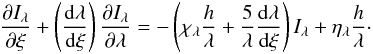 (1)The description of the ∂I/∂λ-discretization for homologous velocity fields has been presented in Baron et al. (2009). We use this discretization method and extend it to include the ∂I/∂t time dependence in the solution of the radiative transfer.
The time-dependent 3D radiative transfer equation along a characteristic is a modification of Eq. (15) in Baron et al. (2009) and given by  (2)where the factor a(t) is simply
  (3)The path length along a characteristic is represented by s, the intensity Iλ,t is a function of the wavelength λ and time t along the characteristic. For the detailed derivation of f(s) and a(s) see Baron et al. (2009).
The fully implicit discretization of Eq. (1) in both wavelength and time is given by
![Mathematical equation: $$ \frac{\dx I_{\lambda}}{\dx s}+\left[ a(s)\frac{\lambda_{l}}{\lambda_{l}-\lambda_{l-1}}+\frac{a(t)}{\Delta t}+4a(s)+\chi_{\lambda}f(s)\right] I_{\lambda ,t} $$](/articles/aa/full_html/2012/10/aa18152-11/aa18152-11-eq15.png)
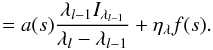 (4)Following Baron et al. (2009), this leads to a modification of the effective optical length
  , which is now defined by
  (5)Baron et al. (2009) chose an unusual sign convention for , which we have restored to its conventional choice. The modified source function Ŝλ is then defined by
  Our restoration of the conventional sign choice for alters the sign of Eq. (7) as compared to Eq. (21) of Baron et al. (2009).
This approach of including time dependence in the 3D RT framework is similar to the first discretization method for the 1D case as described in Jack et al. (2009). The discretization of the ∂I/∂t term modifies the generalized optical depth and adds an additional term to the generalized source function. Please note that the underlying frame differs in the 1D and 3D cases. In the 1D case all momentum quantities are measured by a comoving observer, whereas in the 3D case, only the wavelength is measured by a comoving observer, the momentum angles are measured in the observer’s frame. Additionally as noted in Baron et al. (2009), the path length differs in the 3D case and the 1D case. In the 1D case the path length dsM is that defined by Mihalas (1980), which is not a true distance, whereas our ds is a true distance (Chen et al. 2007). These differences lead to the differences in the equations and in the factor a(t).
3. Test of the implementation
The new extension for time dependence in the solution of the 3D radiative transfer needs to be tested and compared to the results of our time-dependent, 1D spherically symmetric radiative transfer code. We implemented the extension as described above into our MPI parallelized Fortran 95 code described in the previous papers of this series. For all our test calculations, we use a sphere with a gray continuum opacity parameterized by a power law in the continuum optical depth τstd. We interpolate the τstd profile from the 1D grid onto the 3D grid using two-point power-law interpolation. The opacity on the 3D grid is then given by χ = −Δτ/Δr. We use a 3D spherical coordinate system because the results can be directly compared to our 1D spherically symmetric radiation transport code (Hauschildt 1992). The basic model parameters are
-
1.
Inner radius of Rc = 5 × 1010 cm and an outer radius of Rout = 1 × 1011 cm,
-
2.
Optical depth in the range of τmin = 10-6 to τmax = 5,
-
3.
Gray temperature structure with Tmodel = 104 K,
-
4.
Outer boundary condition
 and diffusive inner boundary condition.
 -
5.
We assume an atmosphere in LTE,
-
6.
The atmosphere is static.
For our test calculations, we use a moderately sized 3D grid with nr = 2 ∗ 128 + 1, nφ = 2 ∗ 8 + 1 and nθ = 2 ∗ 4 + 1 points along each axis, for a total of 257 ∗ 9 ∗ 17 ≈ 2 × 10⁴ voxels. See Sect. 3.2 for a detailed explanation why this voxel setup is used. In all tests, we use the full characteristic method for the 3D time-dependent RT solution (Hauschildt & Baron 2006). For the solid angle sampling (θ, φ), we chose a grid of 642 points, which is a reasonable resolution of the spherical coordinate system (Hauschildt & Baron 2009). The time-dependent test calculations are performed with a time step of 10-2 s, unless stated otherwise.
3.1. Constant atmosphere
First, we verify the results for the case of a model atmosphere completely constant in time. The results of the time-dependent RT solution should relax in time to be equal to the time-independent solution.
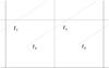 |
Fig. 1 A sketch of two inner voxels and the characteristics of one particular angle, I0 and I1 represent the resulting specific intensities of two characteristics that hit the same voxel. |
To obtain a numerically accurate solution, it is necessary to follow the time derivative of the intensities for each characteristic individually (hereafter: subvoxel method). Previously, the mean intensity of each voxel is a voxel average of the intensities of all characteristics that go through the particular voxel. The characteristics are started either from the innermost or outermost voxels. One specific inner voxel can be hit by many characteristics of the same angle. Figure 1 shows an example of two innermost voxels with the characteristics of one particular angle. Clearly, the voxels are hit by the characteristic that started at the neighboring voxel. This second hit gives an additional and different result for specific intensity for the particular voxel. The intensities are taken at a point of the characteristic that is closest to the center of the voxel. Previously, the mean of all of these intensities has been used to compute the intensity of this particular voxel, Imean = ∑ Ii/n. Using the average of the intensities passing through a given voxel to model the time-dependent intensities results in significant numerical errors, and must therefore be avoided. The explanation is that the difference between the averaged intensity and the individual intensity of a characteristic adds an additional term to the source function. This is completely analogous to the correct treatment of the wavelength derivative in Lagrange frame radiative transfer calculations. In the subvoxel method, all the intensities are saved and used for the individual characteristics. The subvoxel method increases the storage requirements, but this is addressed with a solid-angle domain decomposition method so that the storage requirements per process remain limited.
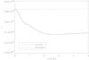 |
Fig. 2 Demonstration of numerical errors. The solid line shows the mean intensity of one outermost voxel for a method that tracks the intensity time derivatives by averaging over a voxel. The mean intensity is inaccurate and then relaxes to the wrong solution. The dot-dashed line shows the results of the subvoxel method, which is numerically much more accurate. |
Figure 2 shows the mean intensity J of one outermost voxel as function of time. Although the atmosphere structure is time independent, the mean intensity changes in time and relaxes to a wrong solution if a numerical method with voxel-averaged time derivatives is used. The errors are on the order of 15% compared to the time independent solution. The mean intensity obtained with the subvoxel method is constant in time and identical to the 3D time-independent solution. Thus, we only use the subvoxel method.
3.2. Perturbations
To see direct effects of the time dependence in the solution of 3D RT problems, we use a setup with a time variable inner boundary condition of our test model atmosphere. These perturbations will then propagate through the model atmosphere by radiation transport in time and finally emerge at the surface of the sphere. We perform the same calculations with our 1D spherically symmetric code and compare the results to the time-dependent 3D spherically symmetric RT.
For all our perturbation tests, we place a “light bulb” at the center of the model atmosphere. This light bulb is just a central source of light inside of the atmosphere. For the first test, the light bulb is switched on and set to (arbitrarily) radiate at 105 times the initial inner boundary intensity. The calculations then track the changes in the 3D (or 1D) radiation field in time.
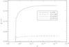 |
Fig. 3 The error of the mean intensity versus τ for different numbers of radial voxels, nr, of a model atmosphere with a light bulb at the inner boundary that has been switched on at the start of the calculations. |
First, we compare the resulting mean intensity J of the time-independent solution to the relaxed time-dependent solution, which should be identical. In Fig. 3, the error in the resulting mean intensity, (Jdep − Jindep)/Jindep, is shown after the atmosphere has relaxed to the new inner boundary condition. Clearly the error is lower when a higher resolution in the radial voxels nr is used. This is equivalent to a higher resolution in the optical depth τ. With nr = 2 ∗ 512 + 1, the error is reduced to below 0.1%. Therefore, we use a large number of voxels for the radial coordinate. Changing the number of voxels for the other coordinates does not affect the resulting mean intensity in this spherically symmetric test.
The test model run with nr = 2 ∗ 512 + 1 has been computed on a supercomputer, where we used 2,048 CPUs. The computation time for this calculation with 500 time steps is about two hours. The storage requirement is about 11 GB and is mainly required for saving all the intensities at a time step. By using a solid-angle domain decomposition, the memory per process required is kept small. For true 3D models the resolution in both the other coordinates nθ and nφ likely also needs to be significantly higher. These calculations are beyond the scope of this work. In future work, we will test our code with a higher resolution in nθ and nφ and apply realistic 3D models to further test our time-dependent extension.
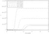 |
Fig. 4 The mean intensity versus time for voxels at different optical depth, τ, of a model atmosphere with a light bulb at the inner boundary that has been switched on at the start of the calculations. |
In Fig. 4, the mean intensity at different layers (radii in the 3D atmosphere) is shown versus time. The additional radiation of the inner light bulb needs time to propagate through the atmosphere. One simple test is to calculate the time the radiation would need at the speed of light to move from the inner to the outermost layer. For the distance of Rout − Rc ≈ 5 × 1010 cm, the radiation needs about ≈ 1.7 s, which is consistent with the result of the 3D radiative transfer as seen in Fig. 4. Figure 5 illustrates the propagation of the radiation “wave” throughout the atmosphere. Here, the mean intensity is plotted against radius for a few snapshots at different times.
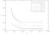 |
Fig. 5 Snapshots of the mean intensity of the atmosphere at different points instants in time. |
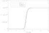 |
Fig. 6 Mean intensity of the outermost radius versus time computed with three different time step choices. |
Another test is to check if the time relaxed result of the time-dependent 3D RT depends on the size of the time steps. The results of this test are shown in Fig. 6, the resulting mean intensities of the outermost layer are plotted for the test case with the light bulb inside computed with three different time step sizes. The change in the mean intensity emerges at the same point in time for all sizes of the time step. However, the shape of the change is different. The explanation is that with a shorter time step, the step function that moves through the atmosphere is better resolved in time.
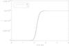 |
Fig. 7 The mean intensity of the outermost radius versus time computed with 3D and 1D time-dependent radiative transfer. |
Another important check is to compare the results of the time-dependent 3D radiative transfer to the results of our 1D spherically symmetric radiative transfer results. The mean intensity of the outermost layer of the 3D and the 1D RT time-dependent calculation is shown in Fig. 7. The test case simulates a light bulb at the inner boundary that has been switched on. The change in the mean intensity emerges at the same point in time, and the final mean intensity is the same.
The next interesting test case is to place a sinusoidally varying light bulb at the center of the sphere and to follow the radiation field in time. This leads to an atmosphere where the mean intensity should vary sinusoidally everywhere. For this test we used a sine wave with a full period of 4 s.
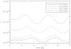 |
Fig. 8 The mean intensity at different optical depths, τ, with a sinusoidally varying light bulb at the center of the sphere. |
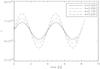 |
Fig. 9 The mean intensity at different optical depths, τ, corrected for the radial time delay. The mean intensities are shifted arbitrarily to better illustrate the smoothing. |
In Fig. 8, the resulting mean intensities for different radii are plotted versus time. It takes about 2 s before the perturbation has moved outwards to affect the outermost layers. The sinusoidally varying mean intensity is then observed in every layer. The phase shift between the inner and outer radii is approximately π, which is about 2 s in time. In Fig. 9, we corrected the resulting sine waves at each optical depth for the radial time delay. We also shifted the mean intensity arbitrarily to directly overlay the sine waves. With this correction for the travel time of the light, there is no additional phase shift. The smoothing of the sine wave as it moves through the atmosphere is also clearly illustrated.
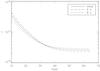 |
Fig. 10 Snapshot of the mean intensity at different phases of the sine wave. |
A snapshot of the mean intensity at different moments in time is shown in Fig. 10. The phase difference between the two snapshots is π.
3.3. Continuum scattering
In this section, we investigate the effects of continuum scattering on the solution of the 3D time dependent radiative transfer. For that, we use a model atmosphere with a low optical depth, so that we can more easily “see” the light bulb at the center. Therefore, we chose for this test: τmin = 10-2 and τmax = 5.
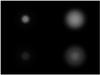 |
Fig. 11 Snapshots of the sphere looking down the pole of the coordinate system. In the right panel side no scattering is considered, while in the left panel the results with scattering are shown. The upper row shows a snapshot at time t = 0 s, and the lower row is at the time of minimum of the sine wave. |
We solved the radiative transfer problem for this model atmosphere both without scattering and for a scattering dominated atmosphere with ϵ = 10-4. A visualization of both spheres is shown in Fig. 11. It shows the image for an observer looking down one pole of the coordinate system. The lefthand panel displays the solution for an atmosphere where no scattering is considered. The outer voxels are dark and not visible to the observer, and the sphere shows strong limb darkening. The righthand panel shows the results with scattering included in the solution of the radiative transfer. The outer voxels of the disk are significantly brighter as the radiation from the light bulb is scattered towards the observer, thus the model showing less limb darkening.
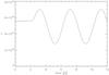 |
Fig. 12 The mean intensity at one outer voxel as a function of time for a sinusoidally varying light bulb at the center of the sphere. |
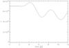 |
Fig. 13 Illustration of the time-dependent mean intensity at the outer boundary for a model with a sinusoidally varying light bulb at the center. In this solution, scattering is considered with ϵ = 10-4. |
We now let the light bulb inside of the sphere vary sinusoidally. The resulting mean intensity versus time is shown in Fig. 12 for one outermost voxel. The mean intensity is varying sinusoidally, as expected. It takes about 2 s for the radiation to travel from the light bulb to the surface. The resulting mean intensity for the solution of radiative transfer considering scattering with ϵ = 10-4 is shown in Fig. 13. Again a sinusoidal variation in intensity is seen at the surface, but it has a smaller amplitude than without scattering. In the presence of scattering, it also takes more time for the radiation to move through the atmosphere. A visualization is shown at Fig. 11. The lower row shows the apparent disk at a minimum of the sine. For the atmosphere where scattering is included, the intensity of the voxels at the outer disk also varies in time.
3.4. A 3D test model
All comparisons with our well-tested 1D spherically symmetric code show that the results of the test models for our implemented time-dependent 3D radiative transfer framework are in good agreement. We now want to verify that our 3D time-dependent extension also works for test cases of a fully 3D test model atmosphere. Unfortunately, we cannot compare these results to our 1D code, but we can discuss whether the results are reasonable.
We again use a spherically symmetric setup in the opacity and radius for the test model atmosphere. For the optical depth, we use a range of τmin = 10-6 to τmax = 5. For the inner radius we chose Rc = 5 × 1010 cm and for the outer radius Rout = 1 × 1011 cm. In this 3D test model, no scattering is considered (ϵ = 1).
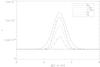 |
Fig. 14 The mean intensity, J, at a ring of outermost voxels (θ = 0) at different times for a test case with an off-center perturbation. |
Since we now want to examine 3D effects, we had to increase our angular resolution. For the following test calculation, we used a setup of nr = 2 ∗ 64 + 1, nθ = 2 ∗ 32 + 1, and nφ = 2 ∗ 64 + 1 voxels. We now place a Gaussian perturbation of the temperature and, therefore, the local source function at an off-center position in the sphere. The center of the Gaussian has a value for the source function 50 times higher than the value of the source function at the center of the sphere and is located 20 voxels away from the center at a radius of 5.69 × 1010cm. The source function is, therefore, given by ![Mathematical equation: \begin{equation} S=S(r)+50 S(r) \exp \left\{-\left[(x-x_0)^2+(y-y_0)^2+(z-z_0)^2\right]/40\right\}, \end{equation}](/articles/aa/full_html/2012/10/aa18152-11/aa18152-11-eq70.png) (8)with a width for the Gaussian perturbation of σ2 = 40. For the first time step, the time-independent model without the perturbation is solved. After the first time step, the perturbation is introduced and remains constant for the rest of the calculation. This means that the resulting mean intensities J will be constant in time after the relaxation process. In Fig. 14, the mean intensity J of one ring of the outermost voxels around the sphere is shown for different times. The perturbation is located inside the sphere at φ = π and θ = 0. The mean intensity J at the initial time t = 0 s is also the result for the non-perturbed
(8)with a width for the Gaussian perturbation of σ2 = 40. For the first time step, the time-independent model without the perturbation is solved. After the first time step, the perturbation is introduced and remains constant for the rest of the calculation. This means that the resulting mean intensities J will be constant in time after the relaxation process. In Fig. 14, the mean intensity J of one ring of the outermost voxels around the sphere is shown for different times. The perturbation is located inside the sphere at φ = π and θ = 0. The mean intensity J at the initial time t = 0 s is also the result for the non-perturbed
model. As expected, the voxels closer to the perturbation have a higher mean intensity J. The intensity then decreases, the farther away the voxel is from the perturbation. On the other side of the sphere, there is no effect on the mean intensities of the outer voxels. It is also clear that it takes more time for the radiation to reach voxels that are farther away from the perturbation.
The calculation for this 3D test model atmosphere run needed about 7000 CPUh. This shows how demanding a fully 3D time-dependent atmosphere computation is, especially for more realistic models in the future. So far, we have only been able to test our time-dependent extension with a gray atmosphere. For realistic models, we need to solve the non-gray radiative transfer equation. For a type Ia supernova model atmosphere in LTE, on the order of 10 000 wavelength points are needed in the computations. The computation time scales roughly linearly with the number of wavelength points.
4. Conclusion
We have implemented direct time dependence into our 3D radiative transfer framework. For best numerical accuracy we used a subvoxel method for the discretized time derivative. We have also shown that it is important to use high resolution in the radial direction. To verify the code, we have calculated the solution for a number of simple parameterized 1D test cases. The inner boundary condition was made time dependent to simulate radiation waves traveling through an atmosphere. All these perturbations move through the atmosphere as expected. We also computed a test case with a sinusoidally varying inner light bulbs. We compared the results of the 3D time-dependent radiative transfer to the results of our well tested 1D spherically symmetric radiative transfer program and found excellent agreement. In a scattering dominated atmosphere, it takes more time for the radiation to move through an atmosphere. We also calculated a fully 3D test case. All tests indicate that the new implementations work as intended.
Acknowledgments
This work was supported in part by the Deutsche Forschungsgemeinschaft (DFG) via the SFB 676, NSF grant AST-0707704, and US DOE Grant DE-FG02-07ER41517. This research used resources of the National Energy Research Scientific Computing Center (NERSC), which is supported by the Office of Science of the US Department of Energy under Contract No. DE-AC02-05CH11231. The computations were carried out at the Höchstleistungs Rechenzentrum Nord (HLRN). We thank all these institutions for generous allocations of computer time. We also thank the anonymous referee for improving the presentation of this work.
References
- Baron, E., & Hauschildt, P. H. 2007, A&A, 468, 255 [NASA ADS] [CrossRef] [EDP Sciences] [Google Scholar]
- Baron, E., Hauschildt, P. H., & Chen, B. 2009, A&A, 498, 987 [NASA ADS] [CrossRef] [EDP Sciences] [Google Scholar]
- Chen, B., Kantowski, R., Baron, E., Knop, S., & Hauschildt, P. H. 2007, MNRAS, 380, 104 [NASA ADS] [CrossRef] [Google Scholar]
- Hauschildt, P. H. 1992, JQSRT, 47, 433 [Google Scholar]
- Hauschildt, P. H., & Baron, E. 2006, A&A, 451, 273 [NASA ADS] [CrossRef] [EDP Sciences] [Google Scholar]
- Hauschildt, P. H., & Baron, E. 2008, A&A, 490, 873 [NASA ADS] [CrossRef] [EDP Sciences] [Google Scholar]
- Hauschildt, P. H., & Baron, E. 2009, A&A, 498, 981 [NASA ADS] [CrossRef] [EDP Sciences] [Google Scholar]
- Hauschildt, P. H., & Baron, E. 2010, A&A, 509, A36 [NASA ADS] [CrossRef] [EDP Sciences] [Google Scholar]
- Hauschildt, P. H., & Baron, E. 2011, A&A, 533, A127 [NASA ADS] [CrossRef] [EDP Sciences] [Google Scholar]
- Jack, D., Hauschildt, P. H., & Baron, E. 2009, A&A, 502, 1043 [NASA ADS] [CrossRef] [EDP Sciences] [Google Scholar]
- Jack, D., Hauschildt, P. H., & Baron, E. 2011, A&A, 528, A141 [NASA ADS] [CrossRef] [EDP Sciences] [Google Scholar]
- Jack, D., Hauschildt, P. H., & Baron, E. 2012, A&A, 538, A132 [NASA ADS] [CrossRef] [EDP Sciences] [Google Scholar]
- Mihalas, D. 1980, ApJ, 237, 574 [NASA ADS] [CrossRef] [Google Scholar]
- Seelmann, A. M., Hauschildt, P. H., & Baron, E. 2010, A&A, 522, A102 [NASA ADS] [CrossRef] [EDP Sciences] [Google Scholar]
- Wang, X., Wang, L., Filippenko, A. V., et al. 2012, ApJ, 749, 126 [NASA ADS] [CrossRef] [Google Scholar]
All Figures
|
Fig. 1 A sketch of two inner voxels and the characteristics of one particular angle, I0 and I1 represent the resulting specific intensities of two characteristics that hit the same voxel. |
| In the text | |
|
Fig. 2 Demonstration of numerical errors. The solid line shows the mean intensity of one outermost voxel for a method that tracks the intensity time derivatives by averaging over a voxel. The mean intensity is inaccurate and then relaxes to the wrong solution. The dot-dashed line shows the results of the subvoxel method, which is numerically much more accurate. |
| In the text | |
|
Fig. 3 The error of the mean intensity versus τ for different numbers of radial voxels, nr, of a model atmosphere with a light bulb at the inner boundary that has been switched on at the start of the calculations. |
| In the text | |
|
Fig. 4 The mean intensity versus time for voxels at different optical depth, τ, of a model atmosphere with a light bulb at the inner boundary that has been switched on at the start of the calculations. |
| In the text | |
|
Fig. 5 Snapshots of the mean intensity of the atmosphere at different points instants in time. |
| In the text | |
|
Fig. 6 Mean intensity of the outermost radius versus time computed with three different time step choices. |
| In the text | |
|
Fig. 7 The mean intensity of the outermost radius versus time computed with 3D and 1D time-dependent radiative transfer. |
| In the text | |
|
Fig. 8 The mean intensity at different optical depths, τ, with a sinusoidally varying light bulb at the center of the sphere. |
| In the text | |
|
Fig. 9 The mean intensity at different optical depths, τ, corrected for the radial time delay. The mean intensities are shifted arbitrarily to better illustrate the smoothing. |
| In the text | |
|
Fig. 10 Snapshot of the mean intensity at different phases of the sine wave. |
| In the text | |
|
Fig. 11 Snapshots of the sphere looking down the pole of the coordinate system. In the right panel side no scattering is considered, while in the left panel the results with scattering are shown. The upper row shows a snapshot at time t = 0 s, and the lower row is at the time of minimum of the sine wave. |
| In the text | |
|
Fig. 12 The mean intensity at one outer voxel as a function of time for a sinusoidally varying light bulb at the center of the sphere. |
| In the text | |
|
Fig. 13 Illustration of the time-dependent mean intensity at the outer boundary for a model with a sinusoidally varying light bulb at the center. In this solution, scattering is considered with ϵ = 10-4. |
| In the text | |
|
Fig. 14 The mean intensity, J, at a ring of outermost voxels (θ = 0) at different times for a test case with an off-center perturbation. |
| In the text | |
Current usage metrics show cumulative count of Article Views (full-text article views including HTML views, PDF and ePub downloads, according to the available data) and Abstracts Views on Vision4Press platform.
Data correspond to usage on the plateform after 2015. The current usage metrics is available 48-96 hours after online publication and is updated daily on week days.
Initial download of the metrics may take a while.