| Issue |
A&A
Volume 544, August 2012
|
|
|---|---|---|
| Article Number | A152 | |
| Number of page(s) | 11 | |
| Section | Stellar structure and evolution | |
| DOI | https://doi.org/10.1051/0004-6361/201219712 | |
| Published online | 24 August 2012 | |
A new visual – near-infrared diagnostic to estimate the metallicity of cluster and field dwarf stars
1 INAF – Osservatorio Astronomico di Roma, via Frascati 33, 00040 Monte Porzio Catone, Italy
e-mail: This email address is being protected from spambots. You need JavaScript enabled to view it.
2 IAC – Instituto de Astrofisica de Canarias, Calle via Lactea, 38200 La Laguna, Tenerife, Spain
e-mail: This email address is being protected from spambots. You need JavaScript enabled to view it.
; This email address is being protected from spambots. You need JavaScript enabled to view it.
3 Department of Astrophysics, University of La Laguna, 38200 La Laguna, Tenerife, Spain
4 Università di Roma Tor Vergata, via della Ricerca Scientifica 1, 00133 Rome, Italy
e-mail: This email address is being protected from spambots. You need JavaScript enabled to view it.
; This email address is being protected from spambots. You need JavaScript enabled to view it.
5 INAF – Osservatorio Astronomico di Collurania, via M. Maggini, 64100 Teramo, Italy
e-mail: This email address is being protected from spambots. You need JavaScript enabled to view it.
Received: 30 May 2012
Accepted: 14 July 2012
Abstract
We present a theoretical calibration of a new metallicity diagnostic based on the Strömgren index m1 and on visual – near-infrared (NIR) colors to estimate the global metal abundance of cluster and field dwarf stars. To perform the metallicity calibration we adopt α-enhanced evolutionary models transformed into the observational plane by using atmosphere models computed adopting the same chemical mixture. We apply the new visual-NIR metallicity-index-color (MIC) relations to two different samples of field dwarfs and we find that the difference between photometric estimates and spectroscopic measurements is on average smaller than 0.1 dex, with a dispersion smaller than σ = 0.3 dex. We apply the same MIC relations to a metal-poor (M 92) and a metal-rich (47 Tuc) globular cluster. We find a peak of −2.01 ± 0.08 (σ = 0.30 dex) and −0.47 ± 0.01 (σ = 0.42 dex), respectively.
Key words: stars: abundances / stars: evolution / stars: Population II / stars: low-mass
© ESO, 2012
1. Introduction
The intermediate-band Strömgren photometric system (Strömgren 1966) has, for stars with spectral types from A to G, several indisputable advantages when compared with broad-band photometric systems.
-
i)
The ability to provide robust estimates of intrinsic stellarparameters such as the metal abundance (them1 = (v − b) − (b − y) index, Anthony-Twarog & Twarog 2000; Hilker 2000; Calamida et al. 2007, hereafter CA07), the surface gravity (the c1 = (u − v) − (v − b) index), and the effective temperature (the Hβ index, Nissen 1988; Olsen 1988; Anthony-Twarog & Twarog 2000). The Hβ index is marginally affected by reddening, and therefore can also be compared to a simple color such as b–y to provide individual estimates of reddening corrections (Nissen & Schuster 1991). The same outcome applies to the reddening free [c1] index, and indeed theoretical and empirical evidence (Stetson 1991; Nissen 1994; Calamida et al. 2005) suggests that a color such as u–y compared to [c1] – which is a temperature index for stars hotter than 8500 K – provides a robust reddening index for blue horizontal branch stars.
-
ii)
The use of the m1/c1 versus color plane can also be safely adopted to distinguish cluster and field stars (Anthony-Twarog & Twarog 2000; Rey et al. 2004; Faria et al. 2007; Adén et al. 2009; Árnadóttir et al. 2010).
-
iii)
Accurate Strömgren photometry can also be adopted to constrain the ensemble properties of stellar populations in complex stellar systems like the Galactic bulge (Feltzing & Gilmore 2000) and the disk (Haywood 2001).
-
iv)
The v filter is strongly affected by two CN molecular absorption bands (λ = 4142, λ = 4215 Å). Stars with an over-abundance of carbon (C) and/or nitrogen (N), i.e. CH- and/or CN-strong stars, will have, at fixed color, a larger m1 value, a fundamental property for identifying stars with different CNO abundances in globular clusters (GCs, CA07, Calamida et al. 2009, 2011).
On the other hand, the Strömgren system presents two relevant drawbacks.
-
i)
The u and v bands have short effective wavelengths, namely λeff = 3450 and λeff = 4110 Å. As a consequence the ability to perform accurate photometry with current CCD detectors is hampered by their reduced sensitivity in this wavelength region.
-
ii)
The intrinsic accuracy of the stellar parameters, estimated using Strömgren indices, strongly depends on the accuracy of the absolute zero-point calibrations. This typically means a precision better than 0.03 mag. This precision could be easily accomplished in the era of photoelectric photometry, but it is not trivial effort in the modern age of CCDs.
The calibration of Strömgren photometric indices to obtain stellar metal abundances is not a new technique. Empirical calibrations based on such a method have been given by Strömgren (1964); Bond (1970); Crawford (1975); Nissen (1981). In these works, most of the stars adopted to perform the calibration are nearby (d ≲ 100 pc) F and early-type G dwarfs, with [Fe/H] > −0.8. The adopted samples include a significant fraction of young and intermediate-age disk stars, and a minority of low-mass, old stars. Moreover, these calibrations are based on differential indices δm1 and δc1, i.e. δm1 = m1,Hyades(β) − m1,star(β), where β stands for Hβ and m1,Hyades(β) is the standard relation between m1 and β for the Hyades given by Crawford (1975) and by Olsen (1984). The δm1 can also be defined with b–y as indipendent parameter, but as pointed out by Crawford, δm1(b − y) is less sensitive to metallicity than δm1β, because the b–y color is also affected by blanketing.
The differential indices δm1 and δc1 have the advantage that they measure mostly metallicity and surface gravity, respectively, and are free of temperature effects. However, they are affected by the uncertainty on the photometric zero-point of the Hyades standard relations and require accurate β photometry.
Olsen (1984) derived a metal abundance calibration using high dispersion spectroscopic measurements of [Fe/H] from Cayrel de Strobel & Bentolila (1983) and new Strömgren photometry for a sample of F, G and K dwarfs (Olsen 1983). Olsen provided a linear solution for δm1(b − y) in the range −0.8 < [Fe/H] < 0.4 for F-G0 dwarfs, and a parabolic solution in the range −2.6 < [Fe/H] < 0.4 for G0-K1 dwarfs. However, only one calibrating star has [Fe/H] < −1.9 and only three have [Fe/H] < −1.5.
Schuster & Nissen (1989, hereafter SN89) performed new intrinsic color and metallicity calibrations based on a sample of 711 high-velocity and metal-poor stars with Strömgren photometry from Schuster & Nissen (1988). The stars have been selected to have spectral types in the range F0-K5, surface gravity 3.4 < log (g) < 5.4 and [Fe/H] abundances are based on high-resolution spectra of Cayrel de Strobel & Bentolila (1983); Cayrel de Strobel et al. (1985); Francois (1986). In addition, these stars have uvby photometry in the system of Olsen (1983, 1984). The SN89 metallicity calibrations are based on the indices m1 and c1 and they are valid in the color range 0.22 < (b − y)0 < 0.59 mag and are reddening dependent.
Haywood (2002) claimed that systematic discrepancies of ~−0.1/0.3 dex affected the SN89 photometric metallicity determinations of metal-rich stars in the quoted color range. They showed that this was a consequence of a mismatch between the standard sequence m1, (b − y) of the Hyades used by SN89 to calibrate their metallicity scale, and the Olsen system. A new calibration was proposed by Haywood (2002), on the basis of an enlarged spectroscopic data set, that makes the SN89 calibration applicable to the Olsen’s photometric catalogs.
Ramírez & Meléndez (2005a) proposed a new metallicity calibration for dwarf stars based on an updated spectroscopic catalog by Cayrel de Strobel et al. (2001) and the m1 and c1 indices, with different equations for three b − y color ranges (0.19 < b − y < 0.35, 0.35 < b − y < 0.50, 0.50 < b − y < 0.80 mag). These relations are valid over a broad metallicity range (−2.5 < [Fe/H] < 0.4) and for log(g) > 3.4.
Árnadóttir et al. (2010, hereafter AR10), based on their new compilation of dwarf stars, tested some of the most recent and/or more popular metallicity calibrations (Olsen 1984; Haywood 2002; Ramírez & Meléndez 2005a, SN89). They found that the calibrations by SN89 and by Ramírez & Meléndez (2005a) perform equally well, but the latter covers a larger parameter space. They suggested to adopt the calibration by Ramírez & Meléndez (2005a) and the calibration by Olsen (1984) for dwarfs redder than b–y = 0.8 mag.
More recently, Casagrande et al. (2011, hereafter CAS11) presented a new empirical metallicity calibration for dwarf stars based on the m1 and c1 indices, covering the metallicity range − 2.0 ≲ [Fe/H] ≲ 0.5 and 0.23 < b − y < 0.63 mag. They validated the new calibration by estimating the metallicity of field dwarfs and open clusters, and showed that they give reliable abundance estimates with a dispersion smaller than 0.1 dex.
All these relations to estimate the metal abundance of dwarf stars are hampered by the presence of molecular CN, CH and NH-bands that affect the Strömgren uvb filters, and in turn the global metallicity estimates. Moreover, the quoted relations include the c1 index, that is based on the u filter. As already mentioned, observations in the u filter are very demanding concerning the telescope time and the photometry in this band is less accurate due to the reduced CCD sensitivity in this wavelength region.
We derive, for the first time, a theoretical calibration of a metallicity diagnostic based on the m1 index and on visual-near-infrared (NIR) colors for dwarf stars. The visual-NIR (y, J, H,K) colors adopted in our new metallicity-index-color (MIC) relations have two clear advantages when compared with optical colors: i) they are not hampered by the presence of CN, CH and NH-bands; ii) strong sensitivity to effective temperature. This means that the quoted molecular bands still affect the MIC relations, but only through the Strömgren m1 index.
The new MIC relations are based on α-enhanced evolutionary models and α-enhanced bolometric corrections and color-temperature transformations and are valid in the metallicity range −2.5 < [Fe/H] < 0.5, and for dwarf stars in the mass range 0.5 < M < 0.85 M⊙ (4.5 < log (g) < 5).
The structure of the current paper is as follows. In Sect. 2 we discuss in detail the photometric catalogs of Galactic globular clusters (GGCs) adopted to validate evolutionary models in the visual-NIR colors. Section 3 deals with the approach adopted to calibrate the visual-NIR MIC relations, while in Sect. 4 we present the different tests we performed to validate the current theoretical calibrations together with the comparison between photometric estimates and spectroscopic measurements of metal abundances. We summarize the results and briefly discuss further improvements and applications of the new MIC relations in Sect. 5.
2. Observations and data reduction
We selected two GGCs, namely M 92 (NGC 6341) and 47 Tuc (NGC 104), to check the plausibility of the theoretical models we adopt to perform the metallicity calibration, since they cover a broad range of metal abundance (−2.31 < [Fe/H] < −0.72, Harris 2003).
Log of the NIR images collected with WFC3 on the HST for the GGC 47 Tuc (Program GO-11677, PI: H. Richer, 11453, PI: B. Hilbert) and M 92 (Program GO-1664, PI: T.M. Brown).
The Strömgren photometric catalog of M 92 (NGC 6341) adopted in this investigation was obtained with images collected with the 2.56 m Nordic Optical Telescope (NOT) on La Palma (Grundahl et al. 2000), while the catalog for 47 Tuc (NGC 104) with images collected with the 1.54 m Danish Telescope on La Silla (ESO, Grundahl et al. 2002).
Data for M 92 were collected during June 1998 and stars from the lists of Olsen (1983, 1984) and Schuster & Nissen (1988) were observed to calibrate the instrumental uvby magnitudes. The total field of view (FoV) is ~4 × 4 arcmin, including the cluster center. The pixel scale is 0 11 per pixel and the seeing ranges between 05 and 10 (for more details see Grundahl et al. 2000, CA07).
Data for 47 Tuc were collected during 10 nights in October 1997, using the Danish Faint Object Spectrograph and Camera. The field of view covered by these data is approximately 11 arcmin across, excluding the cluster center. The pixel scale is 039 per pixel and the seeing ranges between 13 and 22. Approximately 150 different standard stars from the lists of Olsen (1983, 1984) and Schuster & Nissen (1988) were also observed to calibrate the data (for more details see Grundahl et al. 2002, CA07).
We cross-correlated the Strömgren catalogs for the two GGCs with the F110W,F160W NIR photometry collected with the Wide Field Camera 3 (WFC3) on board of the Hubble Space Telescope. The log of the WFC3 images adopted in this investigation is given in Table 1. The images were reduced by using a software package that is based largely on the algorithms described by Anderson & King (2006). Details on this program will be given in a stand-alone paper (Anderson et al., in prep.). The data have been calibrated to Vega adopting the prescriptions by Bedin et al. (2005) and using the current on-line estimates for zero points and encircled energies1. The final catalog for M 92 includes 7219 stars with both NIR and Strömgren photometry, covering a FoV of ≈ 2 × 1 arcmin. The catalog for 47 Tuc includes 12 227 stars overlapping with Strömgren photometry over a region of ≈ 3 × 10 arcmin at a distance of about 12 arcmin from the cluster center.
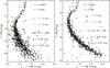 |
Fig. 1 F110W, (y − F110W) CMD for a metal-poor – M 92 (left) – and a metal-rich – 47 Tuc (right) – globular. The green and red solid lines display cluster isochrones. The adopted chemical compositions, age, true distance modulus and reddening are labeled. Tracks were computed by assuming α-enhanced chemical mixtures (PI06) and transformed into the observational plane by adopting atmosphere models with the same α-enhancement. |
Figure 1 shows the F110W, y − F110W CMD for M 92 (left panel) and 47 Tuc (right). Both catalogs are selected in photometric accuracy and in distance from the cluster center. The CMDs display the magnitudes fainter than F110W ≲ 15.5 (M 92) and F110W ≲ 15.0 mag (47 Tuc), since the WFC3 photometry for these clusters is saturated at brighter magnitudes, and we are focusing our attention on main sequence stars. In order to constrain the plausibility of the theoretical framework we adopt for the calibration of the new MIC relations for dwarf stars, we compare current visual-NIR photometry with evolutionary prescriptions. We adopted a true distance modulus of μ = 14.65 mag and a mean reddening of E(B − V) = 0.02 mag for M 92 (Di Cecco et al. 2010), and μ = 13.25 mag and E(B − V) = 0.03 mag for 47 Tuc (Bono et al. 2008). The extinction coefficients are estimated by applying the Cardelli et al. (1989) reddening relations and RV = AV/E(B − V) = 3.1, finding AF110W = 0.32 × AV and E(y − F110W) = 2.12 × E(B − V) mag. The green and red solid lines in Fig. 1 show two isochrones with appropriate ages and chemical compositions, namely Z = 0.0003, Y = 0.245, t = 12 and t = 14 Gyr, and Z = 0.008, Y = 0.256, t = 11 and t = 13 Gyr for M 92 (Di Cecco et al. 2010; Brasseur et al. 2010) and 47 Tuc (Bono et al. 2008), respectively. Isochrones are from the BASTI data base and are based on α-enhanced ([α/Fe] = 0.4) evolutionary models (Pietrinferni et al. 2006, hereafter PI06). Evolutionary prescriptions were transformed into the observational plane by using atmosphere models computed assuming α-enhanced mixtures. Data plotted in Fig. 1 show that theory and observations, within the errors, agree quite well over the entire magnitude range for both clusters.
3. Calibration of new optical-NIR metallicity indices for dwarf stars
Independent MIC relations were derived using cluster isochrones based on α-enhanced evolutionary models (PI06). Theoretical predictions were transformed into the observational plane by adopting bolometric corrections (BCs) and color-temperature relations (CTRs) based on atmosphere models computed assuming the same heavy element abundances (PI06, Castelli & Kurucz 2006). The Vega flux adopted is from Castelli & Kurucz (1994)2. The metallicities used for the calibration of the MIC relations are: Z = 0.0001, 0.0003, 0.0006, 0.001, 0.002, 0.004, 0.01, 0.02 and 0.03. The adopted Z values indicate the global abundance of heavy elements in the chemical mixture, with a solar metal abundance of (Z/X)⊙ = 0.0245.
Figure 2 shows the nine isochrones plotted in different visual-NIR (left) and Strömgren (right) MIC planes. The J, H, K filters where transformed into the 2MASS photometric system by applying the color transformations by Carpenter et al. (2001). Panels a)–c) display the m1 index versus three visual-NIR colors (y − K, y − H, y − J), while the panels d)–f) the m1 index versus three Strömgren colors (u − y, v − y, b − y). The evolutionary phases plotted in this figure range from approximately 4 mag fainter (Md, empty squares) than the main sequence turn-off (MSTO) to 1 mag fainter (Mu, asterisks) than the MSTO. For a metal-intermediate chemical composition (Z = 0.002, Y = 0.248) the quoted limits imply absolute visual magnitudes of MV ≈ 7.8 (M/M⊙ = 0.5) and MV ≈ 5.2 mag (M/M⊙ = 0.75).
Data plotted in Fig. 2 show that the m1 versus visual-NIR colors planes have a stronger sensitivity to metallicity of dwarf stars, when compared with the m1 versus Strömgren colors. The two different sets of MIC relations cover similar m1 values but the visual-NIR colors – panels a)–c) – show a stronger sensitivity in the faint magnitude limit and an almost linear change when moving from metal-poor to metal-rich stellar structures. The Strömgren colors – panels d)–f) – show a minimal sensitivity for stellar structures more metal-rich than [M/H] ≳ −1.0. Moreover and even more importantly, the slopes of the MIC relations based on visual-NIR colors are on average shallower than the MIC relations based on Strömgren colors. This means that the former indices have, at fixed m1 value, a stronger temperature sensitivity.
MIC relations for dwarf stars based on Strömgren colors are affected by the presence of molecular bands, such as CN, CH and NH. As a matter of fact, two strong cyanogen (CN) molecular absorption bands are located at λ = 4142 and λ = 4215 Å, i.e. very close to the effective wavelength of the v filter (λeff = 4110, Δλ = 190 Å). Moreover, the strong CH molecular band located in the Fraunhofer’s G-band (λ = 4300 Å) might affect both the v and the b magnitude. It is noteworthy that the molecular NH band at λ = 3360 Å, and the two CN bands at λ = 3590 and λ = 3883 Å might affect the u (λeff = 3450, Δλ = 300 Å) magnitude (see, e.g. Smith 1987). To decrease the contamination by molecular bands in the color index, we decided to adopt only colors based on the y-band and on the NIR bands in our new calibration of MIC relations. The main advantage of this approach is that the aforementioned molecular bands only affect the Strömgren m1 index.
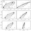 |
Fig. 2 Left panels – m1 vs. y − K plane [panel a)] for isochrones at fixed cluster age (t = 12 Gyr) and different global metallicities ( [M/H] , see labeled values). The evolutionary phases range from ≈ 4 mag fainter (Md, empty squares) than the MSTO to ≈1 mag fainter (Mu, asterisks) than the MSTO. Evolutionary tracks were computed by assuming α-enhanced chemical mixtures (PI06) and transformed into the observational plane by adopting atmosphere models computed assuming the same α-enhancements. The panels b) and c) show similar relations, but in the m1 vs. y − H and in the m1 vs. y − J plane. Right panels – same as the left, but for the m1 vs. u − y [panel d)], m1 vs. v − y [panel e)], m1 vs. b − y [panel f)] planes. |
Multilinear regression coefficients for the Strömgren metallicity index: ![Mathematical equation: \hbox{$m_1 = \alpha\, + \beta\,\feh\ + \gamma\, CI + \delta\, (CI \times m_1) + \epsilon\, CI^2 + \zeta\, m_1^2 + \eta\, (CI^2 \times m_1) + \theta\, (CI \times m_1^2) + \iota\, (CI^2 \times m_1^2) + \kappa\, (CI \times \feh) + \lambda\, (m_1 \times {\rm [Fe/H]})$}](/articles/aa/full_html/2012/08/aa19712-12/aa19712-12-eq125.png) .
.
We derived theoretical MIC relations based on m1 and the y-NIR colors based on WFC3 (F110W,F160W) and 2MASS (J,H,K) bands. Together with the classical m1 index, we also computed independent MIC relations for the reddening-free parameter [m] = m1 + 0.3 × (b − y), to overcome deceptive uncertainties caused by differential reddening. To select the m1 and the [m] values along the individual isochrones we followed the same approach adopted in CA07. A multilinear regression fit was performed to estimate the coefficients of the MIC relations for the m1 and the [m] indices as a function of the five CIs, namely y − F110W, y − F160W, y − J, y − H and y − K: 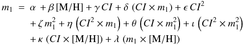 where the symbols have their usual meaning. The adoption of eleven terms, compared to the four terms of the m1 versus Strömgren color calibration for red giants, is due to the nonlinearity of the m1 versus visual-NIR color relations for dwarf stars. To select the form of the analytical relation we followed the forms adopted for the m1 and the hk metallicity index calibrations in CA07 and Calamida et al. (2011), respectively. We performed several tests finding the best solution of the multilinear regression fit when adopting the m1 index as an independent variable. We then selected the solution with the lowest chi-square of the multilinear regression fit. As a further check, we estimated the root mean square (rms) deviations of the fitted points from the fit and the values range between 0.0004 to 0.0012. Moreover, the multi-correlation parameters attain values close to 1. The coefficients of the fits, together with their uncertainties, for the ten MIC relations, are listed in Table 2. The rms values and the multi-correlation parameters of the different relations are listed in the last tow columns.
The above MIC relations are valid in the following color ranges, 0.0 < m1 < 0.6 mag, 0.1 < [m] < 0.8 mag, 1.1 < y − F110W < 1.9 mag, 1.45 < y − F160W < 2.6 mag, 1.1 < y − J < 2.0 mag, 1.1 < y − H < 2.5 mag, and 1.5 < y − K < 2.8 mag, and for dwarf stars in the mass range 0.5 ≲ M ≲ 0.85 M⊙ (4.5 < log (g) < 5).
4. Validation of the new metallicity calibration
4.1. Field dwarf stars
In order to validate the new theoretical calibration of the m1 index based on y-NIR colors for dwarf stars we estimate the metallicity of field dwarfs for which vby photometry, NIR photometry and high-resolution spectroscopy are available. We selected two catalogs from the literature, the former by AR10 includes 451 dwarfs, while the latter by CAS11 includes 1498 dwarfs.
The vby photometry for the stars in the AR10 catalog was retrieved by different studies and transformed into the Strömgren system of Olsen (1993), while the high-resolution spectroscopic abundances were collected from different analysis and homogenized to the spectroscopic system of Valenti & Fischer (2005). The extinction values were estimated by using the reddening map by Schlegel et al. (1998) and modeling the dust in the Galactic disk with a thin exponential disk with a scale-height of ≈ 125 pc (see AR10 for more details). Stars with a reddening E(B − V) < 0.02 mag are assumed to be unreddened and no correction was applied to the photometry of these stars (AR10).
To unredden the m1 index and the colors of the dwarf stars we adopt E(m1) = −0.30 × E(b − y) (Calamida et al. 2007), and E(y − J) = 2.23 × E(B − V), E(y − H) = 2.56 × E(B − V) E(y − K) = 2.75 × E(B − V), estimated assuming the Cardelli et al. (1989) reddening relation and RV = AV/E(B − V) = 3.1.
This sample was cross-correlated with the 2MASS photometric catalog by retrieving for each dwarf star J,H,K-band measurements.
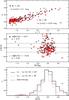 |
Fig. 3 Panel a) selected field dwarf stars from the sample of AR10 plotted in the unreddened m1, y − H plane (Ns = 221, filled dots). Stars selected for σJ,H,K < 0.03 mag are marked with red crosses (Ns = 96). Panel b) difference between photometric and spectroscopic metallicities, Δ [M/H] = ( [M/H] phot − [M/H] spec), plotted versus [M/H] spec for the 221 field dwarfs (filled dots). Photometric metallicities are based on the m1, y − H MIC relation. Panel c) photometric metallicity distribution for the 221 dwarfs obtained with the m1, y − H MIC relation (black solid line), compared to the same distribution but for the selected 96 stars (red dotted) and to the spectroscopic distribution (black dashed). |
We selected, from the AR10 sample, dwarf stars with a measurement of the global metallicity [M/H] from Valenti & Fischer (2005) and with unreddened colors falling inside the color range of current calibrations. The metallicity range covered by our MIC relations is −2.3 < [M/H] < 0.3, but we select stars with −2.5 < [M/H] < 0.5 to account for uncertainties in spectroscopic abundances and in the metallicity scale (Kraft & Ivans 2003). We further select stars in photometric accuracy (σJ,H,K ≤ 0.1 mag), ending up with a sample of 221 field dwarfs. The selected stars are plotted in the m1, y − H plane in panel a) of Fig. 3 (filled dots). Panel b) of the same figure shows the difference between the photometric and the spectroscopic metallicity (Δ [M/H] = ( [M/H] phot − [M/H] spec) for the 221 field dwarf stars as a function of their spectroscopic metal abundances ( [M/H] spec). The observed spread is mainly due to photometric errors and to the uncertainty in the calibration equation, which account for ≈ 0.25 dex, and to spectroscopic measurement errors. Data plotted in this panel show that there is a group of stars with photometric abundances systematically more metal-rich than the spectroscopic ones. To constrain the nature of this drift, we adopted more restrictive selection criteria for the photometry. By selecting stars with σJ,H,K ≤ 0.03 mag, we ended up with a sample of 96 dwarfs (red asterisks), but the outliers almost completely disappear. The mean difference between photometric and spectroscopic abundances was estimated by adopting the biweight algorithm and for m1, y − H MIC relation it is − 0.02 ± 0.02 dex, with σ = 0.30 dex. The same difference, but based on the entire sample of 221 dwarfs is 0.07 ± 0.02 dex, with σ = 0.31 dex. Panel c) of Fig. 3 shows the comparison between the photometric metallicity distribution based on the m1, y − H MIC relation (solid line) for the 221 dwarfs compared to the distribution obtained for the selected 96 dwarfs (red dotted) and the spectroscopic metallicity distribution (dashed). Data indicate that spectroscopic and photometric metallicity distributions agree quite well within an intrinsic dispersion of the order of 0.3 dex. Photometric metallicity distributions estimated by adopting the other MIC relations agree with each other and the mean difference between photometric and spectroscopic abundances for the 96 stars derived averaging the m1, y − J, m1, y − H, m1, y − K relations is − 0.02 ± 0.10 dex, with a mean intrinsic dispersion of σ = 0.31 dex. The difference attains similar values – 0.07 + 0.06 dex, with σ = 0.31 dex – by averaging the MIC relations based on the reddening free metallicity indices ([m], y − J, [m] , y − H, [m], y − K).
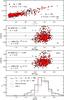 |
Fig. 4 Panel a) selected field dwarf stars from the sample of CAS11 plotted in the unreddened m1, y − H plane (Ns = 488, filled dots). Stars selected for σJ,H,K < 0.03 mag are marked with red crosses (Ns = 185). Panel b) difference between photometric and spectroscopic metallicities, plotted versus the spectroscopic metallicity for the 488 field dwarfs. Photometric metallicities are based on the m1, y − H MIC relation. Panel c) difference between photometric metallicities based on our m1, y − H MIC relation and photometric metallicities by CAS11 plotted versus spectroscopic metallicity. Panel d) photometric metallicity distributions for the 488 dwarfs (black solid line) and for the selected 185 stars (red dotted) obtained with the m1, y − H MIC relation, compared to the photometric distribution by CAS11 (black dotted) and to the spectroscopic distribution (black dashed). |
To further validate the new optical-NIR metallicity calibrations, we also adopt the sample by CAS11. The Strömgren vby photometry for the dwarf stars was retrieved by different studies and transformed into the photometric system of Olsen (1993) by Nordstrom et al. (2004). The interested reader is referred to this paper for more details concerning the sample selection. The high-resolution spectroscopic abundances were collected by CAS11 from three large surveys, namely Valenti & Fischer (2005); Sousa et al. (2008); Bensby et al. (2011). These measurements are consistent with each other and with the homogenized sample of AR10. The final sample includes 1498 dwarf stars with Strömgren photometry and high-resolution spectroscopic measurements. This sample was cross-correlated with the 2MASS catalog and we ended up with a sample of 1135 stars with J,H,K-band photometry. Reddening corrections were applied only to stars with distances larger than 40 pc and with E(b − y) > 0.01 mag, otherwise the extinction was assumed to be vanishing (CAS11). For our analysis we only selected dwarf stars with log (g) > 3.5, −2.5 < [M/H] < 0.5 and in the color range of validity of our metallicity calibration. We further select the sample in photometric accuracy, i.e. σJ,H,K ≤ 0.1 mag, ending up with 488 dwarfs. Panel a) of Fig. 4 shows the selected stars in the m1, y − H plane, while panel b) shows the difference between photometric and spectroscopic metallicity as a function of the spectroscopic metal abundances ( [M/H] spec) for the 488 dwarfs (filled dots). Photometric metallicities are estimated by adopting the m1, y − H MIC relation. The observed spread is mainly due to photometric errors and to the uncertainty in the calibration equation, which account for ≈ 0.2 dex, and to spectroscopic measurement errors. The spectroscopic uncertainty has a mean value of about 0.05 dex, and the difference between metallicities derived in the three spectroscopic surveys adopted ranges from 0.03 to 0.05 dex with a dispersion of ~0.05 dex (see CAS11 and Valenti & Fischer 2005, for more details).
As in the case of AR10 sample, there is a group of stars with photometric metallicities systematically more metal-rich than spectroscopic abundances. Most of them disappear once we apply more restrictive selection criteria in photometric accuracy, σJ,H,K ≤ 0.03 mag, ending up with a sample of 185 dwarfs (red asterisks). On the other hand, the figure shows that for both samples a small shift of photometric metallicities being more metal-poor than spectroscopic measurements is present. The mean difference between photometric and spectroscopic metallicities estimated by using the biweight algorithm for the 185 stars is −0.10 ± 0.02 dex, with σ = 0.22 dex, while for the 488 stars is −0.08 ± 0.02 dex, with σ = 0.25 dex. It is noteworthy that in spite of the shift the shape of the photometric metallicity distributions – solid and red dotted lines in panel d) – agrees quite well with the shape of the spectroscopic one (dashed). A culprit for the systematic shift between photometric and spectroscopic abundances might be an α-enhancement for field dwarfs smaller than the assumed α value. The evolutionary models adopted to perform our theoretical metallicity calibration have been computed assuming [α/Fe] = 0.4. This is the typical enhancement found in cluster stars using high-resolution spectra (Kraft 1994; Gratton et al. 2004). On the other hand, dwarfs in CAS11 sample have [α/Fe] < 0.4, with a median value of [α/Fe] ~ 0.05 (see their Fig. 9). The α-enhanced isochrones have typically redder colors in the m1 versus CI planes compared with scaled-solar models (see Fig. 16 in CA07). Therefore, α-enhanced theoretical MIC relations give more metal-poor metallicity estimates for dwarf stars that are less α-enhanced than cluster stars. This effect decreases when adopting the m1,y − K relation, obtaining a mean difference of 0.0 dex with a dispersion of σ = 0.25 dex for the 185 dwarfs, and of 0.03 dex and σ = 0.32 dex for the 488 dwarfs. Panel c) of Fig. 4 shows the difference between photometric metallicities estimated by adopting our MIC relation m1, y − H and photometric metallicities by CAS11 plotted versus the spectroscopic metal abundances for the two sample of dwarfs. Note that CAS11 estimated photometric [Fe/H] by adopting their fully empirical calibration (see Eqs. (2) or (3) of their paper), and the global metallicity [M/H] by using a Strömgren index (a1) to estimate a proxy of the [α/Fe] abundance of the stars. The mean difference between the photometric metallicities is − 0.10 ± 0.02 dex, with a dispersion of σ = 0.21 dex for the 185 stars, and − 0.08 ± 0.02 dex, with σ = 0.23 dex for the 488 stars. CAS11 metallicity distribution for the sample of 488 dwarfs is also showed in panel d) of Fig. 4. Photometric metallicity estimates obtained by using the other MIC relations agree very well with each other, and the biweight mean difference with the spectroscopic measurements for the 185 stars derived averaging the m1, y − J, m1, y − H, m1, y − K relations is −0.06 ± 0.07 dex, with a mean intrinsic dispersion of σ = 0.22 dex, while is − 0.01 ± 0.06 dex, with σ = 0.25 dex, by averaging the [m] , y − J, [m], y − H, [m] , y − K relations.
In order to constrain the possible dependence on the adopted theoretical framework, we used the evolutionary models publicly available in the Dartmouth database (Dotter et al. 2007, 2008). The cluster isochrones are transformed into the observational plane by using the semi-empirical CTRs by Clem et al. (2004) for the Strömgren colors and the CTRs predicted by PHOENIX atmosphere models for the 2MASS colors (Hauschildt et al. 1999a,b).
We followed the same approach adopted to calibrate the BASTI models. In particular, we selected the same metallicity range, i.e. 0.0001 ≲ Z ≲ 0.03. Six Dartmouth sets of isochrones are available in this metallicity range, i.e. Z = 0.0001, 0.000354, 0.001, 0.00354, 0.01, 0.0352. Note that to account for the fact that the Dartmouth isochrones include gravitational settling of heavy elements, we selected cluster isochrones of 10.5 Gyr. We derived the m1, y − H MIC relation and we applied it to estimate the metallicities of the CAS11 field dwarf sample. The difference between photometric and spectroscopic metallicities, estimated by adopting the biweight algorithm, is 0.20 dex with σ = 0.21 dex. Thus suggesting that the metallicity estimates based on the Dartmouth models are slightly more metal-rich than spectroscopic measurements.
The comparison between the different sets of isochrones have already been discussed in the literature (Dotter et al. 2007, 2008; Pietrinferni et al. 2006, 2009). We compared the two different sets of isochrones in the m1, y − H color–color plane and we found that the Dartmouth models appear, at fixed y − H color, slightly bluer than the BASTI models. The difference might be due to the different sets of CTRs adopted and to the fact that the MIC relations based on the latter set relies on a finer metallicity grid (nine vs. six isochrones).
4.2. Cluster dwarf stars
In order to validate the metallicity calibration based on the visual-WFC3 NIR colors we adopt cluster dwarf stars. We selected two GGCs, namely M 92 and 47 Tuc, with [Fe/H] = −2.31 and [Fe/H] = −0.72, respectively (Harris 2003).
The use of cluster data brings forward three indisputable advantages: a) the evolutionary status (age, effective temperature, surface gravity, stellar mass) of cluster dwarfs is well established; b) the abundance of iron and α-elements is known with high-precision; b) the selected clusters cover a broad range in iron abundance.
Data for these clusters have already been presented in Sect. 2. The top panel of Fig. 5 shows 47 Tuc MS stars plotted in the m1, y − F160W plane. Stars are selected in magnitude, 18.5 < y < 20.5 mag, and for the color ranges of validity of our metallicity calibration, i.e. 1.45 < (y − F160W)0 < 2.6 mag, 0.0 < m10 < 0.6 mag. A further selection is performed in photometric accuracy, σy < 0.05 mag, and in distance from the cluster center, RA < 5.4°. The final sample includes 111 stars, covering a region of 47 Tuc between 5.3 < RA < 5.4°.
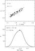 |
Fig. 5 Top: selected MS stars from the GGC 47 Tuc plotted in the m1, y − F160W plane. Bottom: photometric metallicity distribution obtained applying the m1, y − F160W MIC relation for the sample of 47 Tuc MS stars. |
The metallicity distribution of selected 47 Tuc MS stars obtained by applying the m1, y − F160W MIC relation is showed in the bottom panel of Fig. 5. The distribution has been smoothed by applying a Gaussian kernel having a standard deviation equal to the photometric error in the m1 index, following the prescriptions of Calamida et al. (2009). The photometric metallicity distribution is clearly asymmetric and covers more than 1 dex in metal abundance. Fitting the distribution with a Gaussian we found a main peak around [M/H] = −0.51 ( [Fe/H] = −0.86), with a dispersion of σ = 0.29 dex. This estimate is in very good agreement with spectroscopic estimates of 47 Tuc metal abundance from the literature ( [Fe/H] = −0.71 ± 0.05, Rutledge et al. 1997 and [Fe/H] = −0.76 ± 0.02, Carretta et al. 2009). The metallicity distributions obtained by applying the other MIC relations agree with each other, with averaged mean peaks of − 0.47 ± 0.05 dex ( [Fe/H] = −0.82) and a mean intrinsic dispersion of σ = 0.30 dex (m1, y − F110W, m1, y − F160W relations) and of − 0.47 ± 0.02 dex, with σ = 0.28 dex ([m], y − F110W, [m], y − F160W relations).
The large spread in the metallicity distributions might be due to photometric errors. The mean y − F160W and m1 color errors in the selected magnitude bin (18.5 < y < 20.5 mag) are ≈ 0.015 and 0.025 mag, respectively. We simulated the observed m1, y − F160W 47 Tuc color–color plane by assuming isochrones with Z = 0.008, Y = 0.256, t = 11 Gyr (see Sect. 1) in the Strömgren and WFC3 NIR colors. We selected only points in the color ranges of validity of the calibration, i.e. 1.45 < (y − F160W) < 2.6 mag, 0.0 < m1 < 0.6 mag, and added to each point a random error drawn from a Gaussian distribution with sigma equal to the photometric mean error in the selected colors. The metallicities have been estimated from the simulated dwarf sequence and we get a symmetric distribution with a peak at [M/H] = −0.45 and σ = 0.30 dex.
To constrain the possible culprit for the asymmetry in the cluster metallicity distribution we select stars more metal-poor than [M/H] < −0.8 (Ns = 21) according to the distribution obtained by applying the m1, y − F160W relation (Fig. 5), and we check for the presence of spatial distribution trends. We compare the spatial distribution of selected stars with the rest of the sample ( [M/H] ≥ −0.8, Ns = 90) and we do not detect any peculiarity.
Anderson et al. (2009) and Milone et al. (2012) have recently disclosed, based on HST data, the presence of at least two sequences along 47 Tuc MS, corresponding to two different stellar populations with the same iron content, but probably different He and light element abundances. The two stellar populations, defined as “first” and “second” generation have different spatial distributions. The He/N-enriched subsample, i.e. the second generation, is more centrally concentrated and accounts up to ~70% of the cluster population. The photometric metallicity distributions we obtain for the sample of 111 dwarfs of 47 Tuc seem to suggest the presence of stars more metal-poor than the mean cluster metallicity, but our sample is too small to draw firm conclusions.
The top panel of Fig. 6 shows M 92 selected MS stars plotted in the m1, y − F160W plane. The sample is selected in magnitude, 20.0 < y < 20.7 mag, in photometric accuracy, Sharpness < 0.8, and for the color range of validity of our metallicity calibration, ending up with 25 stars. The bottom panel of Fig. 6 shows the smoothed photometric metallicity distribution obtained by applying the m1, y − F160W MIC relation to the sample. The distribution covers more than 2 dex in metallicity and it has an asymmetric shape although less pronounced that in the case of 47 Tuc. By fitting the distribution with a Gaussian we obtain a main peak at [M/H] = −1.88 ( [Fe/H] = −2.23) with a dispersion of σ = 0.42 dex. The metallicity distributions obtained by applying the other MIC relations agree with each other, with averaged mean peaks of −1.85 ± 0.05 dex ([Fe/H] = −2.20) and a mean intrinsic dispersion of σ = 0.43 dex (m1, y − F110W, m1, y − F160W relations) and of −2.17 ± 0.20 dex ( [Fe/H] = −2.52), with σ = 0.35 dex ( [m] , y − F110W, [m] , y − F160W relations). These estimate are in good agreement, within uncertainties, with spectroscopic estimates from the literature ( [Fe/H] = −2.24 ± 0.10, Zinn & West 1984; and [Fe/H] = −2.35 ± 0.05, Carretta et al. 2009).
M 92 shows the typical variations in [C/Fe] and [N/Fe] (Carbon et al. 1982; Langer et al. 1986; Bellman et al. 2001), together with the usual anticorrelations of most GGCs (Pilachowski et al. 1983; Sneden et al. 1991; Kraft 1994). Moreover, preliminary analysis of HST data suggest that also M 92 exhibits multiple sequences in the CMD in close analogy with 47 Tuc (Milone et al., in prep.). On the other hand, most of the spread of the metallicity distribution is due to the large photometric errors of the catalog in this region of the CMD (see also Fig. 1). The mean y − F160W and m1 color errors in the selected magnitude bin (20.0 < y < 20.7 mag) are 0.035 mag and 0.07, with maximum values of 0.11 mag and 0.13 mag, respectively. As in the case of 47 Tuc, we simulated the observed m1, y − F160W color–color plane by assuming isochrones with Z = 0.0003, Y = 0.245, t = 13 Gyr (see Sect. 1) in the Strömgren and WFC3 NIR colors. We selected only points in the color ranges of validity of the calibration, i.e. 1.45 < (y − F160W)0 < 2.6 mag, 0.0 < m10 < 0.6 mag, and added a random error to each magnitude drawn from a Gaussian distribution with sigma equal to the photometric mean error in that band. The metallicities have been estimated from the simulated dwarf sequence and we get a distribution with a large spread, with a peak at [M/H] = −1.50 and σ = 0.45 dex (the adopted isochrones are slightly more metal-rich than M 92).
Therefore the photometric error and the small sample does not allow us to infer the presence of stars with different light-element abundances in the cluster.
5. Conclusions
We have presented a new theoretical metallicity calibration based on the m1 index and on visual-NIR colors to estimate the global metal abundance of cluster and field dwarf stars. We adopted α-enhanced evolutionary models transformed into the observational plane by using atmosphere models with the same chemical mixture to derive the new MIC relations. This is the first time that visual-NIR colors are adopted to estimate photometric metallicities of dwarf stars. The main advantages of the new MIC relations are the following:
-
i)
The molecular bands CH, CN and NH affect them1 index, but the color indices are unaffected by theirpresence.
-
ii)
The metallicity sensitivity is larger in the metal-rich regime, i.e. for [M/H] ≳ −1.0, where isochrones in the m1 versus y – NIR color planes are well separated compared to the same isochrones in the m1 versus Strömgren color planes. The sensitivity is larger also in the metal-poor regime, where isochrones overlap in the m1 versus Strömgren color planes at bluer colors, i.e. for b − y ≤ 0.4 mag.
-
iii)
The slopes of the MIC relations based on visual-NIR colors are on average shallower than the MIC relations based on Strömgren colors. This means that the former indices have, at fixed m1 value, a stronger temperature sensitivity.
-
iv)
They do not include the u filter, which is very time consuming from the observational point of view. Moreover, Strömgren photometry in the u-band is usually less accurate given the reduced sensitivity of CCDs in this wavelength region.
In order to validate the new theoretical metallicity calibration we adopted two sample of field dwarfs with Strömgren and NIR photometry and high-resolution spectroscopy available. The first sample includes 96 dwarfs selected from the study by AR10. The mean difference between photometric and spectroscopic abundance is −0.02 ± 0.10 dex, with a mean intrinsic dispersion of σ = 0.31 dex (m1, y − J, m1, y − H, m1, y − K relations), while is 0.07 ± 0.06 dex, with σ = 0.31 dex ([m], y − J, [m] , y − H, [m], y − K relations).
A further check has been performed by adopting 185 dwarfs selected from the study by CAS11. In this case the mean difference between photometric and spectroscopic abundance is − 0.06 ± 0.07 dex, with a mean intrinsic dispersion of σ = 0.22 dex (m1, y − J, m1, y − H, m1, y − K relations), while is − 0.01 ± 0.06 dex, with σ = 0.25 dex ([m], y − J, [m] , y − H, [m], y − K relations).
The quoted independent comparisons indicate that the new theoretical MIC relations provide accurate metal abundances for field dwarf stars with a dispersion smaller than 0.3 dex.
We tested the calibration by adopting also MS stars of two GGCs covering a broad range in metal abundance, i.e. M 92 ([Fe/H] = −2.31) and 47 Tuc ([Fe/H] = −0.72), for which both Strömgren and WFC3 NIR photometry were available.
We found that the metallicity distributions of 47 Tuc based on the new visual-NIR MIC relations are larger than suggested by spectroscopic measurements of both iron and α-element abundances. Most of the spread is given by photometric errors but a fraction of it, and in particular the asymmetry in the metallicity distribution might be caused by the occurrence of multiple populations in this cluster (Milone et al. 2012). Unfortunately, the stars for which we estimated the metallicity do not have, to our knowledge, spectroscopic measurements of iron, α and light elements. Therefore, we cannot constrain, on a quantitative basis, whether the large spread and the asymmetry in the metallicity distribution of 47 Tuc MS stars is caused by peculiar abundance patterns. According to current estimates photometric errors either in optical or in NIR magnitudes increase the spread in metallicity by at most for 0.30 dex. New medium and high-resolution spectra for the selected cluster MS stars can help us to shed new light on the culprit(s) causing the large spread in metal abundance.
In the case of M 92 the spread of the metallicity distributions is given by the large photometric errors of the catalog at this magnitude level.
We also plan to provide independent calibrations of the new visual-NIR diagnostic by using either semi-empirical CTRs for both Strömgren (Clem et al. 2004) and NIR colors and/or colors predicted by different sets of atmosphere models (PHOENIX, Hautschild et al. 1999a,b; MARCS, Gustafsson et al. 2008) or different sets of evolutionary models (Dotter et al. 2007, 2008; Girardi et al. 2002; VandenBerg et al. 2006).
The complete set of BCs, CTRs and the Vega flux are available at http://wwwuser.oat.ts.astro.it/castelli
Acknowledgments
We acknowledge Luca Casagrande for kindly sending us photometric and spectroscopic data for field dwarfs and for the very useful suggestions that helped us to improve the content of the paper. We thank Santi Cassisi for his constructive suggestions and advices. Support for this work has been provided by the IAC (grant 310394), and the Education and Science Ministry of Spain (grants AYA2007-3E3506, and AYA2010-16717). We acknowledge the referee for his/her pertinent comments and suggestions that helped us to improve the content and the readability of the manuscript.
References
- Anderson, J., & King, I. R. 2006, Instrument Science Report ACS 2006-01 [Google Scholar]
- Anderson, J., Piotto, G., King, I. R., Bedin, L. R., & Guhathakurta, P. 2009, ApJ, 697, L58 [NASA ADS] [CrossRef] [Google Scholar]
- Árnadóttir, A. S., Feltzing, S., & Lundström, I. 2010, A&A, 521, A40 (AR10) [NASA ADS] [CrossRef] [EDP Sciences] [Google Scholar]
- Adén, D., Feltzing, S., Koch, A., et al. 2009, A&A, 506, 1147 [NASA ADS] [CrossRef] [EDP Sciences] [Google Scholar]
- Anthony-Twarog, B. J., & Twarog, B. A. 2000, AJ, 120, 3111 [NASA ADS] [CrossRef] [Google Scholar]
- Bedin, L. R., Cassisi, S., Castelli, F., et al. 2005, MNRAS, 357, 1038 [NASA ADS] [CrossRef] [Google Scholar]
- Bellman, S., Briley, M. M., Smith, G. H., & Claver, C. F. 2001, PASP, 113, 326 [NASA ADS] [CrossRef] [Google Scholar]
- Bensby, T., Adén, D., Meléndez, J., et al. 2011, A&A, 533, A134 [NASA ADS] [CrossRef] [EDP Sciences] [Google Scholar]
- Bond, H. E. 1970, ApJS, 22, 117 [NASA ADS] [CrossRef] [Google Scholar]
- Bono, G. 2008, ApJ, 686, L87 [NASA ADS] [CrossRef] [Google Scholar]
- Brasseur, C. M., Stetson, P. B., VandenBerg, D. A., et al. 2010, AJ, 140, 1672 [NASA ADS] [CrossRef] [Google Scholar]
- Calamida, A., Stetson, P. B., Bono, G., et al. 2005, ApJ, 634, L69 [NASA ADS] [CrossRef] [Google Scholar]
- Calamida, A., Bono, G., Stetson, P. B., et al. 2007, ApJ, 670, 400 (CA07) [NASA ADS] [CrossRef] [Google Scholar]
- Calamida, A., Bono, G., Stetson, P. B., et al. 2009, ApJ, 706, 1277 [NASA ADS] [CrossRef] [Google Scholar]
- Calamida, A., Bono, G., Corsi, C. E., et al. 2011, ApJ, 742, L28 [NASA ADS] [CrossRef] [Google Scholar]
- Carbon, D. F., Romanishin, W., Langer, G. E., et al. 1982, ApJS, 49, 207 [NASA ADS] [CrossRef] [Google Scholar]
- Cardelli, J. A., Clayton, G. C., & Mathis, J. S. 1989, ApJ, 345, 245 [NASA ADS] [CrossRef] [Google Scholar]
- Carpenter, J. M. 2001, AJ, 121, 2851 [NASA ADS] [CrossRef] [Google Scholar]
- Carretta, E., Bragaglia, A., Gratton, R., D’Orazi, V., & Lucatello, S. 2009, A&A, 508, 695 [NASA ADS] [CrossRef] [EDP Sciences] [Google Scholar]
- Casagrande, L., Schönrich, R., Asplund, M., et al. 2011, A&A, 530, A138 (CAS11) [NASA ADS] [CrossRef] [EDP Sciences] [Google Scholar]
- Clem, J. L., Vandenberg, D. A., Grundahl, F., & Bell, R. A. 2004, AJ, 127, 1227 [NASA ADS] [CrossRef] [Google Scholar]
- Crawford, D. L. 1975, AJ, 80, 955 [NASA ADS] [CrossRef] [Google Scholar]
- Di Cecco, A., Becucci, R., Bono, G., et al. 2010, PASP, 122, 991 [NASA ADS] [CrossRef] [Google Scholar]
- Cassisi, S., Salaris, M., Pietrinferni, A., et al. 2008, ApJ, 672, L115 [NASA ADS] [CrossRef] [Google Scholar]
- Castelli, F., & Kurucz, R. L. 1994, A&A, 281, 817 [NASA ADS] [Google Scholar]
- Castelli, F., & Kurucz, R. L. 2006, A&A, 454, 333 [NASA ADS] [CrossRef] [EDP Sciences] [Google Scholar]
- Cayrel de Strobel, G., & Bentolila, C. 1983, A&A, 119, 1 [NASA ADS] [Google Scholar]
- Cayrel de Strobel, G., Bentolila, C., Hauck, B., & Duquennoy, A. 1985, A&AS, 59, 145 [NASA ADS] [Google Scholar]
- Cayrel de Strobel, G., Soubiran, C., & Ralite, N. 2001, A&A, 373, 159 [NASA ADS] [CrossRef] [EDP Sciences] [Google Scholar]
- Dotter, A., Chaboyer, B., Jevremović, D., et al. 2007, AJ, 134, 376 [NASA ADS] [CrossRef] [Google Scholar]
- Dotter, A., Chaboyer, B., Jevremović, D., et al. 2008, ApJS, 178, 89 [NASA ADS] [CrossRef] [Google Scholar]
- Faria, D., Feltzing, S., Lundstrom, I., et al. 2007, A&A, 465, 357 [NASA ADS] [CrossRef] [EDP Sciences] [MathSciNet] [Google Scholar]
- Feltzing, S., & Gilmore, G. 2000, A&A, 355, 949 [NASA ADS] [Google Scholar]
- Francois, P. 1986, A&A, 160, 264 [NASA ADS] [Google Scholar]
- Girardi, L., Bertelli, G., Bressan, A., et al. 2002, A&A, 391, 195 [NASA ADS] [CrossRef] [EDP Sciences] [Google Scholar]
- Gratton, R., Sneden, C., & Carretta, E. 2004, ARA&A, 42, 385 [NASA ADS] [CrossRef] [Google Scholar]
- Grundahl, F., VandenBerg, D. A., Bell, R. A., Andersen, M. I., & Stetson, P. B. 2000, AJ, 120, 1884 [NASA ADS] [CrossRef] [Google Scholar]
- Grundahl, F., Stetson, P. B., & Andersen, M. I. 2002, A&A, 395, 481 [NASA ADS] [CrossRef] [EDP Sciences] [Google Scholar]
- Gustafsson, B., Edvardsson, B., Eriksson, K., et al. 2008, A&A, 486, 951 [NASA ADS] [CrossRef] [EDP Sciences] [Google Scholar]
- Harris, W. E. 2003, Catalog of Parameters for Milky Way Globular Clusters: The Database Hamilton: McMaster Univ., http://physun.physics.mcmaster.ca/~harris/mwgc.dat [Google Scholar]
- Hauschildt, P. H., Allard, F., & Baron, E. 1999a, ApJ, 512, 377 [NASA ADS] [CrossRef] [Google Scholar]
- Hauschildt, P. H., Allard, F., Ferguson, J., Baron, E., & Alexander, D. 1999b, ApJ, 525, 871 [NASA ADS] [CrossRef] [Google Scholar]
- Haywood, M. 2001, MNRAS, 325, 1365 [NASA ADS] [CrossRef] [Google Scholar]
- Haywood, M. 2002, MNRAS, 337, 151 [NASA ADS] [CrossRef] [Google Scholar]
- Hilker, M. 2000, A&A, 355, 994 [NASA ADS] [Google Scholar]
- Kraft, R. P. 1994, PASP, 106, 553 [NASA ADS] [CrossRef] [Google Scholar]
- Kraft, R. P., & Ivans, I. I. 2003, PASP, 115, 143 [NASA ADS] [CrossRef] [Google Scholar]
- Langer, G. E., Kraft, R. P., Carbon, D. F., Friel, E., & Oke, J. B. 1986, PASP, 98, 473 [Google Scholar]
- Milone, A. P., Piotto, G., Bedin, L. R., et al. 2012, ApJ, 744, 58 [NASA ADS] [CrossRef] [Google Scholar]
- Nissen, P. E. 1981, A&A, 97, 145 [NASA ADS] [Google Scholar]
- Nissen, P. E. 1988, A&A, 199, 146 [NASA ADS] [Google Scholar]
- Nissen, P. E. 1994, RMxAA, 29, 129 [Google Scholar]
- Nissen, P. E., & Schuster, W. J. 1991, A&A, 251, 457 [NASA ADS] [Google Scholar]
- Nordström, B., Mayor, M., Andersen, J., et al. 2004, A&A, 418, 989 [NASA ADS] [CrossRef] [EDP Sciences] [Google Scholar]
- Olsen, E. H. 1983, A&AS, 54, 55 [NASA ADS] [Google Scholar]
- Olsen, E. H. 1984, A&AS, 57, 443 [NASA ADS] [Google Scholar]
- Olsen, E. H. 1988, A&A, 189, 173 [NASA ADS] [Google Scholar]
- Olsen, E. H. 1993, A&AS, 102, 89 [NASA ADS] [Google Scholar]
- Pietrinferni, A., Cassisi, S., Salaris, M., & Castelli, F. 2006, ApJ, 642, 697 (PI06) [Google Scholar]
- Pietrinferni, A., Cassisi, S., Salaris, M., Percival, S., & Ferguson, J. W. 2009, ApJ, 697, 275 [NASA ADS] [CrossRef] [Google Scholar]
- Pilachowski, C. A., Bothun, G. D., Olszewski, E. W., & Odell, A. 1983, ApJ, 273, 187 [NASA ADS] [CrossRef] [Google Scholar]
- Ramírez, I., & Meléndez, J. 2005, AJ, 626, 446 [NASA ADS] [CrossRef] [MathSciNet] [Google Scholar]
- Rey, S.-C., Lee, Y.-W., Ree, C.H., et al. 2004, AJ, 127, 958 [NASA ADS] [CrossRef] [Google Scholar]
- Richter, P., Hilker, M., & Richtler, T. 1999, A&A, 350, 476 [NASA ADS] [Google Scholar]
- Rutledge, G. A., Hesser, J. E., Stetson, P. B., et al. 1997, PASP, 109, 907 [NASA ADS] [CrossRef] [Google Scholar]
- Salaris, M., Chieffi, A., & Straniero, O. 1993, ApJ, 414, 580 [NASA ADS] [CrossRef] [Google Scholar]
- Schlegel, D. J., Finkbeiner, D. P., & Davis, M. 1998, ApJ, 500, 525 [NASA ADS] [CrossRef] [Google Scholar]
- Schuster, W. J., & Nissen, P. E. 1988, A&AS, 221, 65 [Google Scholar]
- Schuster, W. J., & Nissen, P. E. 1989, A&AS, 73, 225 (SN89) [Google Scholar]
- Sneden, C., Kraft, R. P., Prosser, C. F., & Langer, G. E. 1991, AJ, 102, 2001 [NASA ADS] [CrossRef] [Google Scholar]
- Sousa, S. G., Santos, N. C., Mayor, M., et al. 2008, A&A, 487, 373 [NASA ADS] [CrossRef] [EDP Sciences] [MathSciNet] [Google Scholar]
- Stetson, P. B. 1991, AJ, 102, 589 [NASA ADS] [CrossRef] [Google Scholar]
- Strömgren, B. 1964, ApNr, 9, 333 [Google Scholar]
- Strömgren, B. 1966, ARA&A, 4, 433 [NASA ADS] [CrossRef] [Google Scholar]
- Valenti, J. A., & Fischer, D. A. 2005, ApJS, 159, 141 [NASA ADS] [CrossRef] [MathSciNet] [Google Scholar]
- VandenBerg, D. A., Bergbusch, P. A., & Dowler, P. D. 2006, ApJS, 162, 375 [NASA ADS] [CrossRef] [MathSciNet] [Google Scholar]
- Zinn, R., & West, M. J. 1984, ApJS, 55, 45 [NASA ADS] [CrossRef] [Google Scholar]
All Tables
Log of the NIR images collected with WFC3 on the HST for the GGC 47 Tuc (Program GO-11677, PI: H. Richer, 11453, PI: B. Hilbert) and M 92 (Program GO-1664, PI: T.M. Brown).
All Figures
|
Fig. 1 F110W, (y − F110W) CMD for a metal-poor – M 92 (left) – and a metal-rich – 47 Tuc (right) – globular. The green and red solid lines display cluster isochrones. The adopted chemical compositions, age, true distance modulus and reddening are labeled. Tracks were computed by assuming α-enhanced chemical mixtures (PI06) and transformed into the observational plane by adopting atmosphere models with the same α-enhancement. |
| In the text | |
|
Fig. 2 Left panels – m1 vs. y − K plane [panel a)] for isochrones at fixed cluster age (t = 12 Gyr) and different global metallicities ( [M/H] , see labeled values). The evolutionary phases range from ≈ 4 mag fainter (Md, empty squares) than the MSTO to ≈1 mag fainter (Mu, asterisks) than the MSTO. Evolutionary tracks were computed by assuming α-enhanced chemical mixtures (PI06) and transformed into the observational plane by adopting atmosphere models computed assuming the same α-enhancements. The panels b) and c) show similar relations, but in the m1 vs. y − H and in the m1 vs. y − J plane. Right panels – same as the left, but for the m1 vs. u − y [panel d)], m1 vs. v − y [panel e)], m1 vs. b − y [panel f)] planes. |
| In the text | |
|
Fig. 3 Panel a) selected field dwarf stars from the sample of AR10 plotted in the unreddened m1, y − H plane (Ns = 221, filled dots). Stars selected for σJ,H,K < 0.03 mag are marked with red crosses (Ns = 96). Panel b) difference between photometric and spectroscopic metallicities, Δ [M/H] = ( [M/H] phot − [M/H] spec), plotted versus [M/H] spec for the 221 field dwarfs (filled dots). Photometric metallicities are based on the m1, y − H MIC relation. Panel c) photometric metallicity distribution for the 221 dwarfs obtained with the m1, y − H MIC relation (black solid line), compared to the same distribution but for the selected 96 stars (red dotted) and to the spectroscopic distribution (black dashed). |
| In the text | |
|
Fig. 4 Panel a) selected field dwarf stars from the sample of CAS11 plotted in the unreddened m1, y − H plane (Ns = 488, filled dots). Stars selected for σJ,H,K < 0.03 mag are marked with red crosses (Ns = 185). Panel b) difference between photometric and spectroscopic metallicities, plotted versus the spectroscopic metallicity for the 488 field dwarfs. Photometric metallicities are based on the m1, y − H MIC relation. Panel c) difference between photometric metallicities based on our m1, y − H MIC relation and photometric metallicities by CAS11 plotted versus spectroscopic metallicity. Panel d) photometric metallicity distributions for the 488 dwarfs (black solid line) and for the selected 185 stars (red dotted) obtained with the m1, y − H MIC relation, compared to the photometric distribution by CAS11 (black dotted) and to the spectroscopic distribution (black dashed). |
| In the text | |
|
Fig. 5 Top: selected MS stars from the GGC 47 Tuc plotted in the m1, y − F160W plane. Bottom: photometric metallicity distribution obtained applying the m1, y − F160W MIC relation for the sample of 47 Tuc MS stars. |
| In the text | |
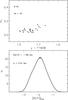 |
Fig. 6 Same ad Fig. 5 but for the GGC M 92. |
| In the text | |
Current usage metrics show cumulative count of Article Views (full-text article views including HTML views, PDF and ePub downloads, according to the available data) and Abstracts Views on Vision4Press platform.
Data correspond to usage on the plateform after 2015. The current usage metrics is available 48-96 hours after online publication and is updated daily on week days.
Initial download of the metrics may take a while.