| Issue |
A&A
Volume 544, August 2012
|
|
|---|---|---|
| Article Number | L9 | |
| Number of page(s) | 5 | |
| Section | Letters | |
| DOI | https://doi.org/10.1051/0004-6361/201219615 | |
| Published online | 06 August 2012 | |
Warm H2O and OH in the disk around the Herbig star HD 163296⋆
1 Max Planck Institut für Extraterrestrische Physik, Giessenbachstrasse 1, 85748 Garching, Germany
e-mail: This email address is being protected from spambots. You need JavaScript enabled to view it.
2 Leiden Observatory, PO Box 9513, 2300 RA Leiden, The Netherlands
3 Kavli Institute for Astronomy and Astrophysics, Yi He Yuan Lu 5, 100871 Beijing, PR China
4 University of Texas at Austin, Department of Astronomy, 2515 Speedway, Stop C1400, Austin TX 78712-1205, USA
5 Max Planck Institute for Astronomy, Königstuhl 17, 69117 Heidelberg, Germany
Received: 16 May 2012
Accepted: 17 July 2012
Abstract
We present observations of far-infrared (50−200 μm) OH and H2O emission of the disk around the Herbig Ae star HD 163296 obtained with Herschel/PACS in the context of the DIGIT key program. In addition to strong [O i] emission, a number of OH doublets and a few weak highly excited lines of H2O are detected. The presence of warm H2O in this Herbig disk is confirmed by a line stacking analysis, enabled by the full PACS spectral scan, and by lines seen in Spitzer data. The line fluxes are analyzed using a local-thermal-equilibrium slab model including line opacity. The H2O column density is 1014−1015 cm-2, and the excitation temperature is 200−300 K, implying warm gas with a density n > 105 cm-3. For OH, we find Nmol of 1014−1015 cm-2 and Tex ~ 300−500 K. For both species, we find an emitting region of r ~ 15−20 AU from the star. We argue that the molecular emission arises from the protoplanetary disk rather than the outflow. This far-infrared detection of both H2O and OH contrasts with near- and mid-infrared observations, which have generally found a lack of water in the inner disk around Herbig AeBe stars owing to the strong photodissociation of H2O. Given the similar column density and emitting region, OH and H2O emission seems to arise from an upper layer of the disk atmosphere of HD 163296, which probes a new reservoir of water. The slightly lower temperature of H2O compared to OH suggests a vertical stratification of the molecular gas with OH located higher and H2O deeper in the disk, consistent with thermo-chemical models.
Key words: protoplanetary disks / stars: variables: T Tauri, Herbig Ae/Be / astrochemistry
Appendices are available in electronic form at http://www.aanda.org
© ESO, 2012
1. Introduction
Water is a key molecule for the chemical and physical evolution of protoplanetary disks. Together with O and OH, it forms the main reservoir of oxygen. The formation of water ice layers on dust grains may improve their sticking behavior and thereby help the coagulation process toward larger particles that ultimately leads to the formation of planetesimals and planets. The growth of icy grains is also likely involved in the delivery of water to planets. Recent observations at near- (~3 μm) and mid-infrared (~10−30 μm) wavelengths have revealed the common presence of hot (T ~ 500−1000 K) water and OH vapor in the atmosphere of T Tauri disks (Salyk et al. 2008; Carr & Najita 2008; Pontoppidan et al. 2010; Mandell et al. 2012). In contrast, disks around the more massive Herbig AeBe stars do not display hot water-vapor emission and appear to be depleted in water molecules (Mandell et al. 2008; Pontoppidan et al. 2010; Fedele et al. 2011). A likely explanation is that hot water is photodissociated by the stronger ultraviolet (UV) radiation emitted by the Herbig stars in the regions of the disks (<a few AU) probed at these wavelengths (e.g. Fedele et al. 2011). In the case of the young eruptive star EX Lupi the, H2O emission is variable as a consequence of the changing UV radiation field (Banzatti et al. 2012).
However, cooler water may survive at greater distance from the star or deeper within these disks, but these regions can only be probed by longer wavelength data. Herschel offers the opportunity to search for these water lines with high sensitivity. Detections of water in disks with Herschel have been reported by Hogerheijde et al. (2011) using HIFI and Riviere-Marichalar et al. (2012) using PACS, but these observations refer only to disks around T Tauri stars.
In this Letter, we report the detection of OH far-infrared emission lines and the signal of warm H2O toward the Herbig Ae star HD 163296 (A1V) at a distance of d = 118 pc (van Leeuwen 2007). The star is isolated with no evidence of a stellar companion and is surrounded by a well-studied disk (e.g., Mannings & Sargent 1997; Grady et al. 2001; Isella et al. 2007). A bipolar microjet and a series of Herbig-Haro knots are observed at optical and UV wavelengths perpendicular to the disk (e.g., Wassell et al. 2006). The disk was recently modeled by Tilling et al. (2012), who also report upper limits to selected OH and H2O lines from PACS data obtained in the GASPS Herschel key program.
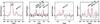 |
Fig. 1 PACS spectrum (continuum-subtracted) of selected lines. The (blue) dashed line indicates the root mean square of the baseline multiplied by three. The presented spectrum has been smoothed (smooth width = two bins) for clarity. The red line is a Gaussian fit to the detected lines. |
2. Observations and data reduction
HD 163296 was observed on April 03 2011 with the PACS instrument (Poglitsch et al. 2010) onboard the Herschel Space Observatory (Pilbratt et al. 2010) as part of the DIGIT key program (KPOT_nevans_1, PI: N. Evans). The target was observed in range spectroscopy mode covering the wavelength range 50−220 μm with R ~ 1000−3000 (obsid: 1342217819, 1342217829). The observations were carried out in chopping/nodding mode with a chopping throw of 6′. The total on-source integration time is 6176 s for the B2A (51−73 μm) and short R1 (70−105 μm) modules and 8360 s for the B2B (70−105 μm) and long R1 (140−220 μm) modules. The data were reduced with HIPE 8.0.2489 using standard calibration files from level 0 to level 2. The data for the two nod positions were reduced separately (oversampling factor = 3, up-sampling factor = 1 to ensure that the noise in each spectral point is independent) and averaged after a flat-field correction.
The spectrum was extracted from the central spaxel (9.4″ square) to optimize the signal-to-noise ratio. Owing to the large point spread function of the telescope, some flux leaks into the other spaxels of the PACS array. To recover the absolute flux level, we applied a correction factor using the spectrum extracted from the central 9 spaxels (3 × 3 extraction): this was performed by fitting a third-order polynomial to each of the two extracted spectra (central spaxel and 3 × 3) and multiplying by a correction defined to be the ratio of these two fits. Finally, the spectrum was scaled so that the spectrum matched the PACS photometry (from Meeus et al., in prep.) at 70 μm and 160 μm.
The line flux (Fline) was measured by fitting a Gaussian function and the uncertainty (σ) was given by the product 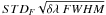 1, where STDF (W m-2 μm-1) is the standard deviation of the (local) spectrum, δλ is the wavelength spacing of the bins (μm), and FWHM is the full width at half maximum of the line (μm).
3. Results
We clearly detect the strong [O i] 63 μm line as well as five OH far-infrared features above 3σ (i.e. having Fline/σ > 3, Table 1). Spectra of selected lines are shown in Fig. 1. The OH lines are readily recognized because of their doublet pattern; only intra-ladder transitions, which have the largest Einstein-A coefficients, are found. In the case of the  doublet at 71 μm, only one of the two lines is detected, although the non-detection of the second line is hardly significant within the noise. Asymmetric line intensities of Λ-doublets are predicted at high temperature (Offer & van Dishoeck 1992), but because of the noise this doublet is not considered in our analysis below.
Three lines of H2O are detected slightly above 3σ (Table 2). The H2O 818−707 line at 63.32 μm is seen not only in our data but also in the GASPS spectrum shown by Tilling et al. (2012), although they do not claim a detection. The H2O 423−312 line at 78.74 μm is seen here with a flux of 1.8 (±0.4) × 10-17 W m-2, while Tilling et al. (2012) report only a 3σ upper limit of 1.5 × 10⁻¹⁷ W m-2. Meeus et al. (2012) claim a detection of far-infrared H2O emission toward this source based on new GASPS data. Pontoppidan et al. (2010) also provide tentative detections of H2O lines in the mid-infrared Spitzer wavelength range. Table 2 summarizes our fluxes and includes the fluxes measured at the position of some (undetected) key H2O lines that are used later in the analysis.
[O i] and OH line fluxes.
H2O line fluxes.
The detected lines have upper level energies over a wide range of values of Eu/k ~ 120−900 K (OH) and Eu/k ~ 400−1300 K (H2O). Most of the lines are detected in the blue part of the spectrum.
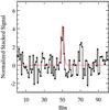 |
Fig. 2 Stacking of 54 H2O lines. Water emission is clearly detected in the stacked spectrum. The integrated signal is SH2O = 7σ. |
3.1. Confirmation of H2O by line stacking
Since only three H2O lines are marginally detected above 3σ, we used the availability of the full DIGIT PACS spectrum to confirm the presence of warm water in this disk through a stacking analysis. Line stacking is commonly used in extragalactic surveys to detect the faint emission lines from the outer regions of galaxies (e.g., Schruba et al. 2011). Warm water has many lines spread throughout the far-infrared wavelength region that can be used for this purpose. In this work, we stacked spectra centered at the location of different H2O lines based on the far-infrared lines detected with PACS toward the protostar NGC 1333 IRAS 4B (Herczeg et al. 2012). The 95−100 μm range is excluded because of spectral leakage (produced by overlap of grating orders). Blended lines are excluded from this analysis and OH and [O i] lines are masked. The remaining number of H2O lines available for the analysis is 54. The stacked spectrum is the weighted average of 54 spectra, each of which is 100 bins wide centered at the position of a water line  , where Fj is the (continuum-subtracted) spectrum centered at the jth water line and wj is the weight of the line. The weight corresponds to
  , where STDj is the standard deviation in the continuum-subtracted spectrum Fj. The lines are stacked in bins because the spectral resolution in velocity space varies but is approximately constant in bins.
The stacked spectrum is shown in Fig. 2. The warm H2O signal is clearly detected and centered on the central bin. The integrated H2O signal is seven times its uncertainty. The false alarm probability (FAP), i.e. the probability of detecting a 7σ signal by stacking random portions of the PACS spectrum, is <0.03% based on 10 000 randomized tests (see Appendix B).
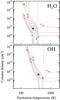 |
Fig. 3 Contours of the reduced χ2 for the slab model of the H2O (upper panel) and OH (lower panel) data. The value of the reduced χ2 is overplotted. The (red) dashed lines provide the radius of the emitting region (10, 20, 30 AU). The star indicates the location of the minimum χ2. |
This analysis confirms the presence of warm H2O in the PACS spectrum of HD 163296. Stacking H2O lines separately in spectra from the two nod positions also yields >3σ detections. The H2O signal is only detected in the central spaxel and not in off-source spaxels. These last two tests exclude the contamination from an extended and/or off-source emission and confirm that the H2O lines detected in the PACS spectrum are associated with HD 163296.
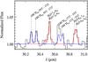 |
Fig. 4 Spitzer/IRS spectrum (continuum-subtracted) of selected lines. The red and blue lines are the best-fit models of H2O and OH, respectively. |
4. Analysis
We analyze the OH and H2O excitation using a uniform slab of gas in local thermal equilibrium (LTE) and including the effect of line opacity (see Appendix A for details). The limited number of lines and their large uncertainties do not warrant a more sophisticated non-LTE treatment. The analysis is based on the data in Tables 1 and 2, including the mid-infrared lines detected with Spitzer/IRS (Pontoppidan et al. 2010). The free parameters of the model are the excitation temperature Tex (K) and the molecular column density Nmol (cm-2). The size of the emitting region, given by its radius r, is not a free parameter since it can be determined uniquely for every given combination of Tex and Nmol. Comparison between models and data is done based on the reduced χ2 values.
The range of models that yields acceptable agreement is shown in Fig. 3. Overplotted are contours for the radius r. For H2O, the data are best-fitted (1σ, p = 68.3%) by models with Tex ~ 200−350 K, and Nmol ~ 1014−1016 cm-2, and r ~ 15−20 AU. For OH, the data are best-fitted by models with Nmol ~ 1014−1015 cm-2, Tex ~ 300−500 K, and r ~ 20 AU. The Spitzer/IRS spectrum of selected lines is shown in Fig. 4, along with the best-fit model.
Further constraints on the H2O column density and temperature come from individual line-flux ratios. In particular, the ratio of far- to mid-infrared lines (e.g. 707−616/761−652) constrains the column density to be > 1014 cm-2. On the other hand, the ratio 818−707/808−717 constrains the upper limit to the H2O column density to be 2 × 1015 cm-2. We also note that models with higher column density produce several H2O lines that are not detected in the PACS and IRS spectra. The ratio 818−707/909−818 constrains the temperature to be < 300 K.
5. Discussion
The primary result of this Letter is a detected signal of H2O, in addition to OH, toward a Herbig star. The H2O emitting region is found to be 15−20 AU in size, demonstrating that H2O can survive the UV radiation further away from the star, while likely being photodissociated in the inner part of the disk.
Given that a bipolar microjet is known to be associated with HD 163296 (Wassell et al. 2006), the question arises of whether the far-infrared molecular line emission presented here indeed arises from the disk or whether it comes from such a jet. There are several arguments in favor of the disk. First, we note that HD 163296 is isolated and not associated with a molecular cloud. No evidence of a molecular outflow has been reported to date (e.g. Bae et al. 2011). Second, the spectrally resolved CO J = 3−2 line in the sub-millimeter shows the characteristic double-peaked profile of gas in Keplerian rotation (Thi et al. 2001; Dent et al. 2005). At much shorter wavelengths (4.7 μm), the CO ro-vibrational emission lines are also characterized by a double-peaked profile (Salyk et al. 2011). Thus, there is no hint of any significant small- or large-scale molecular outflow in these data that could dominate the PACS emission. Third, the PACS data show no evidence of extended/off-source emission beyond the central spaxel, not even for the strong [O i] 63 μm line, which places the warm H2O within 500 AU of the central star.
The inferred OH and H2O excitation temperatures of several hundred Kelvin indicate warm emitting regions. The high critical densities of the H2O lines, nc ≥ 107 cm-3, implies that the density of the gas should also be high (n ≳ 105 cm-3, e.g. Herczeg et al. 2012). These conditions and the arguments above suggest that the OH and H2O emission arises from the atmosphere of the disk associated with HD 163296 at radial distances > 10 AU from the star.
If we assumed that the OH/H2O far-infrared lines are emitted by the disk, which zone would this emission trace? Models of the water chemistry in Herbig disks suggest at least three chemically distinct zones (e.g., Woitke et al. 2009; Glassgold et al. 2009; Walsh et al. 2010, 2012; Vasyunin et al. 2011; Najita et al. 2011): (i) an inner-disk water reservoir ( ≲ few AU) with a chemistry close to LTE; (ii) a cold water belt at large distances ( ≳ 50 AU) where gaseous H2O results primarily from photodesorption of water ice; and (iii) hot water layers at both intermediate distances of 1−30 AU and medium heights with water formation driven by high-temperature neutral-neutral reactions. The derived parameters for our OH and H2O lines are consistent with the existence of zone (iii) (see also Tilling et al. 2012); zone (i) is probed by the near-infrared data and zone (ii) can be targeted by HIFI observations of low-J lines. Thus, the PACS data reveal that there is an additional water reservoir in disks.
6. Conclusions
We have presented new Herschel/PACS observations of the disk around the Herbig Ae star HD 163296. We have detected far-infrared lines of warm OH and H2O toward this Herbig star. The presence of warm H2O is confirmed by a line stacking analysis (7σ detection) enabled by the full PACS spectral scan. Our LTE slab-model analysis including optical depth effects indicates emission from the intermediate radii of the disk. Combined with near-infrared and sub-millimeter data, the oxygen chemistry can now be probed over the entire disk range.
Online material
Appendix A: Slab model
For an optically thin line from a point-like source, the flux can be written by
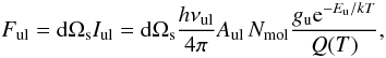 (A.1)for the solid angle of the source dΩs, the line frequency νul, the Einstein-A coefficient Aul, the molecular column density Nmol, the statistical weight of the upper level gu, the energy of the upper level Eu, and the partition function Q(T). The solid angle of the emitting region can be written as dΩs ≡ πr2/d2, for the radius of the emitting region r and a distance of d = 118 pc to HD 163296. For an optically thick line, the integrated intensity is obtained from
 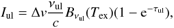 (A.2)where the opacity at the line center is
 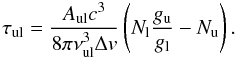 (A.3)The (thermal) width of the lines is assumed to be Δv ~ 1 km s-1, which is appropriate for gas at several hundred K and we assume a simple square-like line profile as e.g. used in the RADEX code (van der Tak et al. 2007).
Appendix B: False alarm probability of water detection in the stacked spectrum
We performed a simulation to measure the probability of detecting a signal with an integrated value, S > 7σ. This provides the false alarm probability (FAP) of a detection based on the stacked spectrum. We performed 10 000 random stackings of 54 (equal
to the number of water lines) parts of the PACS spectrum of HD 163296. After 10 000 iterations, we measured the distribution of the ratio of the integrated signal to its uncertainty (measured as in Sect. 3.1). We masked the bins containing H2O, OH, and [O i] emission. Figure B.1 shows the distribution of S/σ. The distribution is well-fitted by a Gaussian function (red line,  ), centered (as expected) at S/σ = 0 (i.e. an equal number of positive and negative peaks). The number of occurrences with S/σ > 7 is less than thee, which corresponds to FAP < 0.03% according to Bayesian statistics.
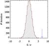 |
Fig. B.1 Distribution of S/σ after 10,000 random stackings of 54 parts of the PACS spectrum of HD 163296. The red line shows the Gaussian fit. The arrow indicates the location of the H2O signal (Fig. 2). |
This formula comes directly from the error propagation of the sum Σi(Fi), where Fi is the flux of the ith spectral bin.
References
- Bae, J.-H., Kim, K.-T., Youn, S.-Y., et al. 2011, ApJS, 196, 21 [NASA ADS] [CrossRef] [Google Scholar]
- Banzatti, A., Meyer, M. R., Bruderer, S., et al. 2012, ApJ, 745, 90 [NASA ADS] [CrossRef] [Google Scholar]
- Carr, J. S., & Najita, J. R. 2008, Science, 319, 1504 [NASA ADS] [CrossRef] [PubMed] [Google Scholar]
- Dent, W. R. F., Greaves, J. S., & Coulson, I. M. 2005, MNRAS, 359, 663 [NASA ADS] [CrossRef] [Google Scholar]
- Fedele, D., Pascucci, I., Brittain, S., et al. 2011, ApJ, 732, 106 [NASA ADS] [CrossRef] [Google Scholar]
- Glassgold, A. E., Meijerink, R., & Najita, J. R. 2009, ApJ, 701, 142 [NASA ADS] [CrossRef] [Google Scholar]
- Grady, C. A., Polomski, E. F., Henning, T., et al. 2001, AJ, 122, 3396 [NASA ADS] [CrossRef] [Google Scholar]
- Herczeg, G. J., Karska, A., Bruderer, S., et al. 2012, A&A, 540, A84 [NASA ADS] [CrossRef] [EDP Sciences] [Google Scholar]
- Hogerheijde, M. R., Bergin, E. A., Brinch, C., et al. 2011, Science, 334, 338 [NASA ADS] [CrossRef] [PubMed] [Google Scholar]
- Isella, A., Testi, L., Natta, A., et al. 2007, A&A, 469, 213 [CrossRef] [EDP Sciences] [Google Scholar]
- Mandell, A. M., Mumma, M. J., Blake, G. A., et al. 2008, ApJ, 681, L25 [NASA ADS] [CrossRef] [Google Scholar]
- Mandell, A. M., Bast, J., van Dishoeck, E. F., et al. 2012, ApJ, 747, 92 [Google Scholar]
- Mannings, V., & Sargent, A. I. 1997, ApJ, 490, 792 [NASA ADS] [CrossRef] [Google Scholar]
- Meeus, G., Montesinos, B., Mendigutia, I., et al. 2012, A&A, 544, A78 [NASA ADS] [CrossRef] [EDP Sciences] [Google Scholar]
- Najita, J. R., Ádámkovics, M., & Glassgold, A. E. 2011, ApJ, 743, 147 [NASA ADS] [CrossRef] [Google Scholar]
- Offer, A. R., & van Dishoeck, E. F. 1992, MNRAS, 257, 377 [NASA ADS] [Google Scholar]
- Pilbratt, G. L., Riedinger, J. R., Passvogel, T., et al. 2010, A&A, 518, L1 [CrossRef] [EDP Sciences] [Google Scholar]
- Poglitsch, A., Waelkens, C., Geis, N., et al. 2010, A&A, 518, L2 [NASA ADS] [CrossRef] [EDP Sciences] [Google Scholar]
- Pontoppidan, K. M., Salyk, C., Blake, G. A., et al. 2010, ApJ, 720, 887 [NASA ADS] [CrossRef] [Google Scholar]
- Riviere-Marichalar, P., Ménard, F., Thi, W. F., et al. 2012, A&A, 538, L3 [NASA ADS] [CrossRef] [EDP Sciences] [Google Scholar]
- Salyk, C., Pontoppidan, K. M., Blake, G. A., et al. 2008, ApJ, 676, L49 [NASA ADS] [CrossRef] [Google Scholar]
- Salyk, C., Blake, G. A., Boogert, A. C. A., & Brown, J. M. 2011, ApJ, 743, 112 [NASA ADS] [CrossRef] [Google Scholar]
- Schruba, A., Leroy, A. K., Walter, F., et al. 2011, AJ, 142, 37 [NASA ADS] [CrossRef] [Google Scholar]
- Thi, W. F., van Dishoeck, E. F., Blake, G. A., et al. 2001, ApJ, 561, 1074 [NASA ADS] [CrossRef] [Google Scholar]
- Tilling, I., Woitke, P., Meeus, G., et al. 2012, A&A, 538, A20 [NASA ADS] [CrossRef] [EDP Sciences] [Google Scholar]
- van der Tak, F. F. S., Black, J. H., Schöier, F. L., Jansen, D. J., & van Dishoeck, E. F. 2007, A&A, 468, 627 [NASA ADS] [CrossRef] [EDP Sciences] [Google Scholar]
- van Leeuwen, F. 2007, A&A, 474, 653 [NASA ADS] [CrossRef] [EDP Sciences] [Google Scholar]
- Vasyunin, A. I., Wiebe, D. S., Birnstiel, T., et al. 2011, ApJ, 727, 76 [NASA ADS] [CrossRef] [Google Scholar]
- Walsh, C., Millar, T. J., & Nomura, H. 2010, ApJ, 722, 1607 [NASA ADS] [CrossRef] [Google Scholar]
- Walsh, C., Nomura, H., Millar, T. J., & Aikawa, Y. 2012, ApJ, 747, 114 [NASA ADS] [CrossRef] [Google Scholar]
- Wassell, E. J., Grady, C. A., Woodgate, B., Kimble, R. A., & Bruhweiler, F. C. 2006, ApJ, 650, 985 [NASA ADS] [CrossRef] [Google Scholar]
- Woitke, P., Kamp, I., & Thi, W. 2009, A&A, 501, 383 [NASA ADS] [CrossRef] [EDP Sciences] [Google Scholar]
All Tables
All Figures
|
Fig. 1 PACS spectrum (continuum-subtracted) of selected lines. The (blue) dashed line indicates the root mean square of the baseline multiplied by three. The presented spectrum has been smoothed (smooth width = two bins) for clarity. The red line is a Gaussian fit to the detected lines. |
| In the text | |
|
Fig. 2 Stacking of 54 H2O lines. Water emission is clearly detected in the stacked spectrum. The integrated signal is SH2O = 7σ. |
| In the text | |
|
Fig. 3 Contours of the reduced χ2 for the slab model of the H2O (upper panel) and OH (lower panel) data. The value of the reduced χ2 is overplotted. The (red) dashed lines provide the radius of the emitting region (10, 20, 30 AU). The star indicates the location of the minimum χ2. |
| In the text | |
|
Fig. 4 Spitzer/IRS spectrum (continuum-subtracted) of selected lines. The red and blue lines are the best-fit models of H2O and OH, respectively. |
| In the text | |
|
Fig. B.1 Distribution of S/σ after 10,000 random stackings of 54 parts of the PACS spectrum of HD 163296. The red line shows the Gaussian fit. The arrow indicates the location of the H2O signal (Fig. 2). |
| In the text | |
Current usage metrics show cumulative count of Article Views (full-text article views including HTML views, PDF and ePub downloads, according to the available data) and Abstracts Views on Vision4Press platform.
Data correspond to usage on the plateform after 2015. The current usage metrics is available 48-96 hours after online publication and is updated daily on week days.
Initial download of the metrics may take a while.