| Issue |
A&A
Volume 544, August 2012
|
|
|---|---|---|
| Article Number | A4 | |
| Number of page(s) | 5 | |
| Section | Astronomical instrumentation | |
| DOI | https://doi.org/10.1051/0004-6361/201219399 | |
| Published online | 19 July 2012 | |
A critical evaluation of the principal component analysis detection of polarized signatures using real stellar data
Université de Toulouse, UPS-Observatoire Midi-Pyrénées, Irap, 31028
Toulouse, France CNRS, Institut de Recherche en Astrophysique et
Planétologie, 14 Av. E.
Belin, 31400
Toulouse, France
e-mail: This email address is being protected from spambots. You need JavaScript enabled to view it.
Received:
12
April
2012
Accepted:
22
June
2012
Abstract
The general context of this study is the post-processing of multiline spectropolarimetric observations of stars, and in particular the numerical analysis techniques aiming at detecting and characterizing polarized signatures. Using real observational data, we compare and clarify several points concerning various methods of analysis. We applied and compared the results of simple line addition, least-squares deconvolution, and denoising by principal component analysis to polarized stellar spectra available from the TBLegacy database of the Narval spectropolarimeter. This comparison of various approaches of distinct sophistication levels allows us to make a safe choice for the next implementation of on-line post-processing of our unique database for the stellar physics community.
Key words: methods: data analysis / polarization / stars: magnetic field / astronomical databases: miscellaneous
© ESO, 2012
1. Introduction
This study is concerned with the post-processing of multiline spectropolarimetric measurements, and in particular of stellar data. We focus on data collected since 2006 with the Narval spectropolarimeter mounted at the 2-m aperture Télescope Bernard Lyot (TBL) located at the summit of the Pic du Midi de Bigorre (France). We investigate, in particular, the capabilities of the principal component analysis (PCA) on observations made with Narval.
The PCA has been regularly used in solar spectropolarimetry during the last decade (see e.g., Rees et al. 2000; Skumanich & López Ariste 2002). Its main purpose was to provide an alternative way of inverting spectropolarimetric data to determine the vector magnetic field present in various solar features, from sunspots to solar prominences (see e.g., López Ariste & Casini 2002).
For stellar data, PCA-based denoising of spectral lines was first presented by Caroll et al. (2007). It was subsequently tested on data taken with the SOFIN spectrograph at the NOT telescope. This procedure was mainly aimed at performing Zeeman-Doppler imaging (ZDI; see Semel 1989) from temporal sequences of individual spectral lines, instead of using pseudo-profiles such as those that are commonly computed by least-squares deconvolution (LSD; see Donati et al. 1997; Kochukhov et al. 2010, for a recent review and discussion). Martínez González et al. (2008) discussed in detail the capabilities of PCA denoising of solar and stellar spectropolarimetric data, using synthetic data. These authors also provided some comments on the relationship between PCA denoising, line addition, and least-squares deconvolution. More recently, Ramírez Vélez et al. (2010) proposed another PCA-based method, coupled to ZDI, which was applied to a very limited set of observational data taken both at the AAT telescope with the SemelPol spectropolarimeter, and with Narval at the TBL.
Here we revisit some details of PCA denoising and the analysis of observational spectropolarimetric data. We discuss the practical capabilities of this approach in more detail. Comparisons with LSD and the so-called (simple) line addition (SLA; Semel et al. 2009) methods are also discussed.
2. The source of data
We used Narval data available from the public database TBLegacy1. Narval is a state-of-the-art spectropolarimeter operating in the 0.38−1 μm spectral domain, with a spectral resolution of 65 000 in its polarimetric mode. It is an improved copy, adapted to the 2-m TBL telescope, of the Espadons spectropolarimeter, in operations since 2004 at the 3.6-m aperture CFHT telescope (see Donati et al. 2006, for further technical details).
The TBLegacy database is operational since 2007. It is at the present time the largest on-line archive of high-resolution polarization spectra. It hosts data that were taken at the 2-m TBL telescope since December 2006. So far, more than 70 000 spectra have been made available, for more than 370 distinct targets all over the Hertzsprung-Russell diagram. More than 13 000 polarized spectra are also available, mostly for circular polarization (linear polarization data are very seldom still and amount to a few hundreds spectra, but they are equally available). By default, the latter is the usual circular polarization V(λ)/Ic normalized to the local continuum intensity.
At the present time, the TBLegacy database provides no more than Stokes I or V/Ic spectra calibrated in wavelength. Stokes I data are either normalized to the local continuum or not. In a next step, further post-processing of these spectra will be proposed on-line to users and the relevant software will be made fully available to the community. This will concern the simple line addition and the least-squares deconvolution standard procedures that we used in the present study, together with PCA denoising.
3. Numerical procedures
3.1. The matrix of observations
Observations obtained from TBLegacy are basically Stokes I(λ) or V(λ). They consist of a very large array of about 200 000 elements covering the whole spectral domain observable by Narval. The main task of building the matrix of observations O is to split the multiline observations vs. wavelength into Nobs elementary profiles, each of them centered at a given wavelength and projected onto a common velocity grid. This velocity grid is an a priori data set that we adopt in our numerical procedure. The choice of this grid of velocities depends on the spectral sampling of the original set of data – for the Narval data it is about 1.8 km s-1 – as well as on the target nature, for the considered velocity range (typically between ± 120 and ± 200 km s-1). Practically we deal with Nv velocity bins of about 102, while I or V original data (sampled in wavelength) are recast into Nobs elementary v-sampled profiles, where Nobs is about 103−104, depending on the spectral type of the target.
The transformation of the original data requires the help of a supplementary file, usually called “mask” which consists of the list of all the wavelengths at rest, λ0, of the spectral lines expected to be present in the observations of a given spectral type of stars. For all cases discussed hereafter, we used mask files widely used by the community that are built from the VALD database (Piskunov et al. 1995; resources for this study have been kindly provided to us by E. Alecian). In general, these mask files contain additional information about each spectral line, in particular their line depression, di, and effective Landé factors, gi, required by LSD (see next section).
Therefore, given a proper mask and a velocity grid, it is quite easy and straightforward to transform I(λ) or V(λ) data into Nobs individual I(v) or V(v) profiles, in accordance with the Doppler-Fizeau effect and the well-known relationship  (1)where δλ = (λ − λ0), which is computed from the original data (see also Sect. 2.1 in Ramírez Vélez et al. 2010).
This operation results in the construction of a (Nobs, Nv) rectangular matrix of observations O, which will now be used in different ways.
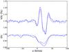 |
Fig. 1 Comparison between LSD (full lines) and SLA (dashed lines) I/Ic and V/Ic pseudo-line profiles for II Peg observations of August 2008. Stokes V profiles have been shifted by 1.1 so the largest amplitude lobe is about 0.1% of Ic for LSD. P1 profiles (dot-dashed) both for I/Ic and V/Ic resulting from the PCA analysis of the data are also displayed for comparison purpose. |
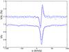 |
Fig. 2 Same as Fig. 1 but for ε Eri observations of February 2007. Stokes V profiles have been shifted by 1.1 and multiplied by 3, so the largest amplitude lobe is about 0.05% of Ic for LSD. |
3.2. Simple line addition vs. LSD
For a wealth of data in TBLegacy, down to polarized signatures V/Ic of about 0.01%, the pseudo-profiles resulting from the simple line addition (or, to be more precise, the unweighted, or arithmetic mean) of the Nobs individual spectral lines of O are very meaningful, both from the standpoints of the detection and of the characterization (i.e., the proper determination of its shape and amplitudes) of the polarized signature carried by the multiline, but noisy, observations. Moreover, SLA profiles are very similar to those obtained from least-squares deconvolution. This was indeed mentioned and discussed in the very instructive, but unfortunately overlooked, recent article of Semel et al. (2009). Nevertheless, to the best of our knowledge, no direct comparisons between LSD and SLA profiles obtained with real data such as Narval’s, have been published yet.
To remedy that, in Figs. 1 and 2, we display LSD and SLA pseudo-profiles obtained directly by computing a simple average of all rows of the O matrix constructed from the same set of observations of the RS CVn star II Peg, made in August 2008. The LSD profiles for Stokes I have been computed using weights ωI = di normalized to the arithmetic mean of the considered central line depressions di. Those for Stokes V were computed for weights ωV = giλ0,idi normalized to the arithmetic mean of the ωV’s. Also, no line depth cut-off criterium was adopted there (provided that depressions are, originally, greater than, or equal to, 10% of the continuum). Considerations and recommendations about the question of LSD weights definition (and especially their normalization) and line depth cut-off criterium can be found in Kochukhov et al. (2010). These authors revealed some lack of discipline in the community of LSD users and subsequent articles still fail, unfortunately, to provide details about the exact procedure that was applied to data – see e.g., Kochukhov et al. (2011) or Donati et al. (2011). To conclude on these points, we again recommend this community to carefully read Semel et al. (2009) and, especially, their Sect. 2.3 dedicated to the statistical properties of (LSD) weights.
For II Peg, we considered about 6600 wavelengths in the mask, covering a 400−1000 nm range, using VALD data for a Teff = 5000 K, a surface gravity of log g = 3.0 cgs, and solar abundances. Concerning this choice of stellar parameters, Berdyugina et al. (1998) determined Teff = 4600 K and log g = 3.2 cgs. However, Teff as high as 5250 K are still reported by VizieR. As can be seen in Fig. 1, the respective shapes of I/Ic and V/Ic are well recovered, both by LSD and SLA, and they are indeed very similar. Amplitudes of the I/Ic and V/Ic LSD pseudo-profiles appear to be systematically slightly larger than SLA ones. However, this is not going to significantly impair any subsequent determination of the mean line-of-sight magnetic field usually made, assuming the weak-field regime of the Zeeman effect, using the center of gravity method (Rees & Semel 1979, and references therein).
We noticed similar effects, displayed in Fig. 2, using observations of the K2V star ε Eri made in February 2007 with Narval. For that case, and after inspecting all VizieR resources, we adopted a Teff = 5000 K and a surface gravity of log g = 4.5 cgs (and solar abundances) mask (see also Koleva & Vazdekis 2012).
Using a test version of TBLegacy currently under development2, we have been able to verify indeed how similar SLA and LSD signatures are, from the analysis of many other cases including magnetic stars hotter than those discussed in this article.
3.3. Principal component analysis
Following Martínez González et al. (2008), we built the cross-product matrix, C = OTO, and computed its eigenvalues si and eigenvectors ei (hereafter, eigenprofiles). Hereafter, we call Oj(v) the observation made at wavelength index j, and we omit the dependance in v of each of these individual profiles. No physical assumption about the line formation process or the origin of the polarization signals are required for the PCA analysis we have carried out.
As demonstrated by Martínez González et al. (2008) with their Figs. 1, without any noise (or a limited amount of it – this is the case for Stokes I data from TBLegacy, for instance), the examination of the sequence of eigenvalues si of C shows that a few of them will dominate, sometimes by orders of magnitudes as compared to the lowest ones. However, for significant noise levels, as will be the case hereafter for Stokes V data, the sequence of si is in general very slowly decreasing – see e.g., Fig. 6.
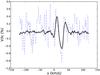 |
Fig. 3 Example of PCA denoising: the original noisy signal Oj(v) (dashed line) for the 612.2 nm line of Ca i, is displayed, together with its projection onto the eigenprofile of matrix C associated with the highest eigenvalue, Pj,1 (full thick line). This last profile already bears a shape very similar to the SLA (or LSD) pseudo-profiles obtained with the whole set of observations, which are displayed in Fig. 1. |
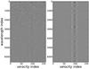 |
Fig. 4 Comparison between the original map of the matrix of observations O (left) and the map of the Pj,1 (right), for II Peg observations of August 2008. The efficiency of the PCA denoising is obvious at almost all wavelengths. |
Even though the sequence of eigenvalues si is very slowly decreasing for most of Stokes V data from TBLegacy, we first tried PCA denoising by computing  (2)for k = 1. For the wavelength index j corresponding to the strong magnetically sensitive 612.2 nm line of Ca i, Fig. 3 shows the efficiency of PCA denoising using only the projection onto the eigenprofile e1 associated to the highest eigenvalue s1. In that case, it is quite obvious that, for this level of signal-to-noise ratio the gain provided by the PCA denoising procedure is significant enough, and potentially allows for the detection of a meaningful polarized signature buried in noise. Moreover, it is easy to notice that the single Pj,1 denoised profile displayed in Fig. 3 already bears a shape very similar to the SLA (or LSD) pseudo-profiles obtained from the whole set of observations, as displayed in Fig. 1.
The efficiency of PCA denoising at all wavelengths can also be seen in Fig. 4 where we displayed images of the observations matrix O (left) in comparison with the matrix of the Pj,1’s (right). In that case, clear polarized signatures emerge almost at all observed wavelengths. It also opens the possibility of a direct exploitation of single line data, instead of a pseudo-profile combining all multiline signatures. The same is true for ε Eri data, for instance, even though its SLA (or LSD) signature is significantly fainter than II Peg’s.
4. Comparison with SLA and LSD
We have shown with the previous examples how PCA denoising can be efficient on real stellar data. It can be very useful for detection purposes but could it offer an alternative to LSD or SLA methods?
The case of ε Eri is interesting in the sense that its polarization signature is less complex but has a much smaller amplitude than that of II Peg. Both LSD and SLA pseudo-line profiles, that is,  (3)show a clear antisymmetric V/Ic profile with amplitudes of a negative and positive lobe of about 0.04−0.05%, and spanning over a Δv ≈ 30 km s-1 spectral range. But this signature, recovered with two distinct methods, is not fully recovered when we consider just the mean of the projection of Oj onto the eigenprofile e1 only. The resulting mean profile is still about a factor of 2 smaller than the amplitude of
  and the lobes are also wider than the ones of LSD or SLA pseudo-profiles – see again Fig. 2. Beyond the detection capability of PCA-based denoising, this poses the additional question of the proper characterization of the “most common” polarization signal content of the multiline observations.
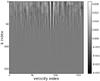 |
Fig. 5 Map of the ( |

To investigate this point, we built a map displayed in Fig. 5, constructed from the successive differences between  (4)and . It is quite clear that about 50 eigenprofiles should be taken into account to recover, from a PCA analysis, a pseudo-line comparable to the SLA (i.e., ) or LSD ones. This result is clearly contradicts the comments made in Sect. 5.1 of Martínez González et al. (2008) about P1 and LSD or SLA pseudo-profiles, using noisy but synthetic data. Indeed, PCA denoising can be made equivalent to the line addition technique, as well as to least-squares deconvolution, but for the TBLegacy data we had been using in that study, at the price of considering a set of eigenprofiles and not the only one associated with the highest eigenvalue of C (and similar behaviors were noticed for II Peg and ε Eri data).
To understand this behavior, it can be worthwhile to analyze, in addition to the polarization data, the so-called “null” spectra, N(λ), which come along with standard Narval (and Espadons) data. It is indeed customary now in stellar spectropolarimetry to proceed with a double beam-exchange method which consists of recording a sequence of four sub-exposures associated to two distinct and opposite polarization states (see e.g., Semel & Li 1996). N profiles result from a combination of sub-exposures, similar to the one used for the extraction of the polarization signal, but this in contrast removes any polarization signal of astrophysical origin. Its main usage is for the eventual detection of any spurious signal in the data that may corrupt the astrophysical signal. However, for clean observations (i.e., when N(λ) is structureless), it basically contains noise, at the same level as the one which remains in the polarized spectra.
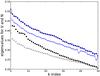 |
Fig. 6 Successive eigenvalues of the cross-correlation matrices computed from the V (dotted lines) and the N (crossed lines) data of II Peg (discontinuous lines) and ε Eri (continous lines) from TBLegacy respectively. Eigenvalues for ε Eri were magnified by a factor of 10. |
The number of eigenprofiles to consider for the reconstructed Pk to be comparable to LSD or SLA pseudo-profiles is roughly given by the index at which the sequences of eigenvalues of V and N, respectively, do overlap. Figure 6 displays two sets of eigenvalues, which overlap indeed for k ≈ 50 in these cases. II Peg data is represented by discontinuous lines, while ε Eri data is represented by continous lines (note also that for this latter set of data, eigenvalues were magnified by a factor of 10). In both cases, V-eigenvalues correspond to dotted lines while cross symbols denote N-eigenvalues. The same kind of empirical criteria was put forward by Martínez González et al. (2008) during their discussion about respective PCA analyses of a “correlated” (synthetic) data set and another one of uncorrelated (Gaussian) noise.
In summary, the simultaneous PCA analysis of V and N allows for (a) the detection of a polarized signature in the data, if the condition  (5)is satisfied, and (b) the characterization of a single representative signature, similar to LSD or SLA pseudo-profiles, which can be made considering projections of the original data onto a number of eigenprofiles, which will be given by this index at which the two sequences of eigenvalues
  and
and  do overlap.
5. Intrinsinc dimension of the dataset
We finally evaluate the intrinsic dimensionality of our main II Peg and ε Eri data sets, following the analysis given in Asensio Ramos et al. (2007), which was illustrated with synthetic data and solar spectropolarimetric observations. To this end, we computed maximum-likelihood dimension estimators  for different values n of neighbors, for each of the profiles contained in the observations matrix O.
We adopted the formula modified by MacKay & Ghahramani (2005)3 after the initial work of Levina & Bickel (2005). For the II Peg and ε Eri data we analyzed, values for appear to be in a range about 38−48, for n ranging from 3 to 75. This is quite consistent with our PCA analysis of Pk vs. , showing that our noisy data force us to consider more eigenprofiles than a priori expected, according to Martínez González et al. (2008).
6. Conclusion
We have experimented with different methods of analysis of multiline polarized spectra of stars. We have shown, using real data, that the simple line addition technique (Semel et al. 2009) allows computing pseudo-profiles very similar to those computed by least-squares deconvolution. It is also much simpler to implement and it requires fewer external input data, which makes it both simple and efficient, and therefore very suitable for the implementation of a standard post-processing tool for the TBLegacy database content.
From our study, LSD does not show any clear advantage on SLA. Furthermore, its systematic use for stellar spectropolarimetric databases would require, for the sake of interoperability, the set-up of a specific protocol concerning the line depth cut-off criteria and the normalization of weights used for Stokes I and V data processing.
We have also applied PCA denoising to real (and noisy) observational data, which proved to be very efficient indeed. We have shown that it can provide an alternative to SLA or LSD post-processing methods, for the characterization of the polarization content of the multiline observations, once the necessary number of eigenprofiles of the cross-product matrix of the observations have been carefully estimated. This can be derived from the combined PCA analysis of V and N data. Finally, and this also holds for SLA, it is in principle equally applicable to all kinds of polarization signals, whatever their physical origin
or observed state of polarization, circular or linear, which was observed.
The (Python) software implemented for this analysis will be made public, although it is already available upon request to the author.
http://www.inference.phy.cam.ac.uk/mackay/dimension/ – See also Eq. (5) in Asensio Ramos et al. (2007).
Acknowledgments
This research has made use of the VizieR catalogue access tool, CDS, Strasbourg, France. The original description of the VizieR service was published in A&AS, 143, 23. Narval data were provided by the Cnrs/Insu Bass2000-CDAB datacenter operated by the Université Paul Sabatier, Toulouse-OMP (Tarbes, France; http://tblegacy.bagn.obs-mip.fr/).
References
- Asensio Ramos, A., Socas-Navarro, H., López Ariste, A., & Martínez González, M. J. 2007, ApJ, 660, 1690 [NASA ADS] [CrossRef] [Google Scholar]
- Berdyugina, S. V., Jankov, S., Ilyin, I., Tuominen, I., & Fekel, F. C. 1998, A&A, 334, 863 [NASA ADS] [Google Scholar]
- Carroll, T. A., Kopf, M., Ilyin, I., & Strassmeier, K. G. 2007, Astron. Nachr., 328, 1043 [NASA ADS] [CrossRef] [Google Scholar]
- Donati, J.-F., Semel, M., Carter, B. D., Rees, D. E., & Collier Cameron, A. 1997, MNRAS, 291, 658 [NASA ADS] [CrossRef] [MathSciNet] [Google Scholar]
- Donati, J.-F., Catala, C., Landstreet, J., & Petit, P. 2006, Solar Polarization 4, eds. Casini, & Lites, ASP Conf. Ser., 358, 362 [Google Scholar]
- Donati, J.-F., Gregory, S. G., Alencar, S. H. P., et al. 2011, MNRAS, 417, 472 [NASA ADS] [CrossRef] [Google Scholar]
- Kochukhov, O., Makaganiuk, V., & Piskunov, N. 2010, A&A, 524, A5 [NASA ADS] [CrossRef] [EDP Sciences] [Google Scholar]
- Kochukhov, O., Makaganiuk, V., Piskunov, N., et al. 2011, ApJ, 732, 19 [Google Scholar]
- Koleva, M., & Vazdekis, A. 2012, A&A, 538, A143 [NASA ADS] [CrossRef] [EDP Sciences] [Google Scholar]
- Levina, E., & Bickel, P. J. 2005, Advances in Neural Information Processing Systems, eds. Saul, Weiss, & Bottou, 17 [Google Scholar]
- López Ariste, A., & Casini, R. 2002, ApJ, 575, 529 [NASA ADS] [CrossRef] [Google Scholar]
- Martínez González, M. J., Asensio Ramos, A., Carroll, T. A., et al. 2008, A&A, 486, 637 [NASA ADS] [CrossRef] [EDP Sciences] [Google Scholar]
- Piskunov, N. E., Kupka, F., Ryabchikova, T. A., Weiss, W. W., & Jeffery, C. S. 1995, A&AS, 112, 525 [NASA ADS] [Google Scholar]
- Ramírez Vélez, J. C., Semel, M., Stift, M., et al. 2010, A&A, 512, A6 [NASA ADS] [CrossRef] [EDP Sciences] [Google Scholar]
- Rees, D., & Semel, M. 1979, A&A, 74, 1 [NASA ADS] [Google Scholar]
- Rees, D., López Ariste, A., Thatcher, J., & Semel, M. 2000, A&A, 355, 759 [NASA ADS] [Google Scholar]
- Semel, M. 1989, A&A, 225, 456 [NASA ADS] [Google Scholar]
- Semel, M., & Li, J. 1996, Sol. Phys., 164, 417 [NASA ADS] [CrossRef] [Google Scholar]
- Semel, M., Ramírez Vélez, J. C., Martínez González, M. J., et al. 2009, A&A, 504, 1003 [NASA ADS] [CrossRef] [EDP Sciences] [Google Scholar]
- Skumanich, A., & López Ariste, A. 2002, ApJ, 570, 379 [NASA ADS] [CrossRef] [Google Scholar]
All Figures
|
Fig. 1 Comparison between LSD (full lines) and SLA (dashed lines) I/Ic and V/Ic pseudo-line profiles for II Peg observations of August 2008. Stokes V profiles have been shifted by 1.1 so the largest amplitude lobe is about 0.1% of Ic for LSD. P1 profiles (dot-dashed) both for I/Ic and V/Ic resulting from the PCA analysis of the data are also displayed for comparison purpose. |
| In the text | |
|
Fig. 2 Same as Fig. 1 but for ε Eri observations of February 2007. Stokes V profiles have been shifted by 1.1 and multiplied by 3, so the largest amplitude lobe is about 0.05% of Ic for LSD. |
| In the text | |
|
Fig. 3 Example of PCA denoising: the original noisy signal Oj(v) (dashed line) for the 612.2 nm line of Ca i, is displayed, together with its projection onto the eigenprofile of matrix C associated with the highest eigenvalue, Pj,1 (full thick line). This last profile already bears a shape very similar to the SLA (or LSD) pseudo-profiles obtained with the whole set of observations, which are displayed in Fig. 1. |
| In the text | |
|
Fig. 4 Comparison between the original map of the matrix of observations O (left) and the map of the Pj,1 (right), for II Peg observations of August 2008. The efficiency of the PCA denoising is obvious at almost all wavelengths. |
| In the text | |
|
Fig. 5 Map of the ( |
| In the text | |
|
Fig. 6 Successive eigenvalues of the cross-correlation matrices computed from the V (dotted lines) and the N (crossed lines) data of II Peg (discontinuous lines) and ε Eri (continous lines) from TBLegacy respectively. Eigenvalues for ε Eri were magnified by a factor of 10. |
| In the text | |
Current usage metrics show cumulative count of Article Views (full-text article views including HTML views, PDF and ePub downloads, according to the available data) and Abstracts Views on Vision4Press platform.
Data correspond to usage on the plateform after 2015. The current usage metrics is available 48-96 hours after online publication and is updated daily on week days.
Initial download of the metrics may take a while.