| Issue |
A&A
Volume 544, August 2012
|
|
|---|---|---|
| Article Number | A37 | |
| Number of page(s) | 28 | |
| Section | Extragalactic astronomy | |
| DOI | https://doi.org/10.1051/0004-6361/201218888 | |
| Published online | 26 July 2012 | |
Intra-night optical variability of core dominated radio quasars: the role of optical polarization⋆
1 National Centre for Radio Astrophysics/TIFR, Pune University Campus, 411 007 Pune, India
e-mail: This email address is being protected from spambots. You need JavaScript enabled to view it.
2 Aryabhatta Research Institute of Observational Sciences (ARIES), Manora Peak, 263 129 Naini Tal, India
3 Department of Physics, The College of New Jersey, PO Box 2718, Ewing, NJ 08628-0718, USA
4 Indian Institute of Astrophysics (IIA) Bangalore 560 034, India
Received: 26 January 2012
Accepted: 10 May 2012
Abstract
Context. Rapid variations in optical flux are seen in many quasars and all blazars. The amount of variability in different classes of active galactic nuclei has been studied extensively but many questions remain unanswered.
Aims. We present the results of a long-term programme to investigate the intra-night optical variability (INOV) of powerful flat spectrum radio core-dominated quasars (CDQs), with a focus on probing the relationship of INOV to the degree of optical polarization.
Methods. We observed a sample of 16 bright CDQs showing strong broad optical emission lines and consisting of both high and low optical polarization quasars (HPCDQs and LPCDQs). In this first systematic study of its kind, we employed the 104-cm Sampurnanand telescope, the 201-cm Himalayan Chandra telescope and the 200-cm IUCAA-Girawali Observatory telescope, to carry out R-band monitoring on a total of 47 nights. Using the CCD as an N-star photometer to densely monitor each quasar for a minimum duration of about 4 h per night, INOV exceeding ~1–2 per cent could be reliably detected. Combining these INOV data with those taken from the literature, after ensuring conformity with the basic selection criteria we adopted for the 16 CDQs monitored by us, we were able to increase the sample size to 21 CDQs (12 LPCDQs and 9 HPCDQs) monitored on a total of 73 nights.
Results. As the existence of a prominent flat-spectrum radio core signifies that strong relativistic beaming is present in all these CDQs, the definitions of the two sets differ primarily in fractional optical polarization, with the LPCDQs showing a very low median Pop ≃ 0.4 per cent. Our study yields an INOV duty cycle (DC) of ~28 per cent for the LPCDQs and ~68 percent for HPCDQs. If only strong INOV with fractional amplitude above 3 per cent is considered, the corresponding DCs are ~7 per cent and ~40 per cent, respectively.
Conclusions. From this strong contrast between the two classes of luminous, relativistically beamed quasars, it is apparent that relativistic beaming is normally not a sufficient condition for strong INOV and a high optical polarization is the other necessary condition. Moreover, the correlation is found to persist for many years after the polarization measurements were made. Some possible implications of this result are pointed out, particularly in the context of the recently detected rapid γ-ray variability of blazars.
Key words: quasars: general / galaxies: jets
Figs. 1–4, 6, 7, and Table 2 are only available in electronic form at http://www.aanda.org
© ESO, 2012
1. Introduction
The occurrence of intranight optical variability (INOV), or microvariability, among quasars, particularly their more active subset called blazars, is now well documented in the literature (e.g., Miller et al. 1989; Jang & Miller 1995, 1997; Romero et al. 1997, 2002; Gopal-Krishna et al. 2003, 2011; Sagar et al. 2004; Stalin et al. 2004a,b, 2005; Gupta et al. 2005, 2008; Rani et al. 2010; Goyal et al. 2010). Considerable uncertainty persists, however, about the underlying physical mechanism and even from a purely observational perspective contrasting claims have been made (reviewed, e.g., by Wiita 2006; Wagner & Witzel 1995). While some observers find INOV to be more dramatic during the optically bright phase of a blazar (e.g., Osterman-Meyer et al. 2009), the opposite has been concluded in another study (Carini 1990). Moreover, some authors have even reported that INOV is more likely to occur when the long-term flux is undergoing a change, rather than at some specific flux levels (e.g., Howard et al. 2004; Mihov et al. 2008).
The LPCDQ and HPCDQ samples studied in the present work$.
In the prior publications under the present long-term programme (e.g., Gopal-Krishna et al. 2003; Stalin et al. 2004a,b; 2005; Sagar et al. 2004), an attempt was made to find clues about the INOV phenomenon by determining and comparing the INOV characteristics of four major classes of powerful active galactic nuclei (AGN). These classes are: “low-frequency-peaked” BL Lacs (LBLs, see, e.g., Table 1 of Abdo et al. 2010) whose synchrotron emission peaks in the IR/optical range, radio core-dominated quasars (CDQs) mostly of the low optical polarization type (LPCDQs), radio lobe-dominated quasars (LDQs) and radio-quiet quasars (RQQs). The study was based on fairly densely sampled intranight R-band differential light curves of duration ≳ 4 h per night for every single AGN and a minimum of 3 nights for each AGN (totalling 113 nights on a 1-m telescope), all processed in a uniform way. This study showed that strong INOV (with fractional variability amplitude ψ > 3 per cent) is exhibited almost exclusively by LBLs and possibly HPCDQs, the high optical polarization subset of CDQs, both together termed blazars (e.g., Angel & Stockmann 1980; Wills et al. 1992; Urry & Padovani 1995), and that the duty cycle of such strong INOV is around 50% (Gopal-Krishna et al. 2003; Stalin et al. 2004a; Sagar et al. 2004; also, Carini et al. 2007), very similar to the value recently estimated for the subset of blazars detected at TeV energies (Gopal-Krishna et al. 2011). In contrast, the other two classes of radio-loud AGN, namely LDQs and LPCDQs, were found to exhibit only low-level INOV and that too with a small duty cycle of only around 10–15%, which is akin to the INOV behaviour exhibited by RQQs (Stalin et al. 2004a,b; also, Ramírez et al. 2009).
These findings suggest that radio loudness (even if associated with relativistic beaming, as likely in the case of LPCDQs) is not a critical factor for the low-level INOV. Here it may be recalled that a similarity between the INOV duty cycles of RQQs and core-dominated quasars had also been noted by de Diego et al. (1998). However, an assessment of their result is rendered difficult due to the fact that many objects in their sample of 17 radio-loud quasars are actually not core-dominated but, instead, have steep radio spectra and are therefore lobe-dominated; moreover, that study is based on rather sparcely sampled light curves.
A major shortcoming of our afore-mentioned INOV program has been that out of the 5 CDQs monitored, only one is a high optical polarization quasar (HPCDQ). This precluded a probe into the role of optical polarization in the INOV phenomenon. The main purpose of the present study is to rectify this situation, by monitoring a set of CDQs which is not only larger in size, but is also a balanced mix of HPCDQs showing high optical polarization with Pop > 3 per cent (the canonical benchmark for blazars, Moore & Stockmann 1981; Moore & Stockman 1984; Stockman et al. 1984; Nartallo et al. 1998; Wills et al. 1992) and their non-blazar counterparts, the “low polarization core-dominated quasars” (LPCDQs). It may be recalled that even though Pop of LPCDQs nearly always remains below ~2% (Stockman et al. 1984; Schmidt & Smith 2000), some contribution from blazar activity cannot be excluded (e.g., Schmidt & Smith 2000; Czerny et al. 2008; Chand et al. 2009). A famous example is the nearby LPCDQ 3C 273, a superluminal source whose Pop always remains below 3% and yet its sensitive photo-polarimetry has revealed a “mini-blazar” component (Impey et al. 1989; Wills 1989; also, Lister & Smith 2000; Schmidt & Smith 2000). In rare instances, the “mini-blazar” component may undergo a strong flaring, as exemplified by the quasar 1633 + 382; known to have Pop < 3 per cent all along, it was found in February 1999 to be strongly polarized with Pop = 7.0 ± 0.5 per cent, confirming its transformation to a bona-fide blazar (Lister & Smith 2000 and references therein). Thus, while in general the possibility that Pop of a blazar might occasionally dip below 3% (e.g., Moore & Stockman 1984; Lister & Smith 2000) should be kept in mind, the division at Pop = 3% to discriminate between LPCDQs and HPCDQs, as adopted here, remains largely valid and is consistent with many previous studies (e.g., Algaba et al. 2011).
Historically, rapid flux variability, high fractional polarization and radio-core dominance (i.e., a flat radio spectrum) have all been regarded as different facets of blazar activity which, in turn, is believed to be associated with a relativistically beamed jet of nonthermal radiation. Starting from the discovery of a strong correlation between radio core dominance and Pop (Impey et al. 1991; Wills et al. 1992; also, Lister & Smith 2000; Fan & Zhang 2003), a flat/inverted radio spectrum of a quasar has often been deemed adequate for classifying it as a blazar (e.g., Maraschi & Tavecchio 2003; Meyer et al. 2011). Some authors have even termed FSRQs as “strong line blazars” (e.g., Perlman et al. 2008), echoing the inference reached in Wills et al. (1992) that high optical polarization quasars and flat-spectrum (core-dominated) quasars are essentially the “same objects”. The question specifically examined here is how the rapid optical continuum variability (on intranight time scale) relates to the two blazar indicators, namely, optical polarization and radio core-dominance.
In spite of the vast literature exploring the inter-relationships among the aforementioned major AGN classes, namely LBLs, HPCDQs, LPCDQs and RQQs, the picture remains unclear. One extreme suggestion bearing on the issue of “radio loudness dichotomy” of quasars (e.g., Ivezić et al. 2002) is based on an analogy with the galactic micro-quasars. It has been argued that a given quasar becomes radio loud when it moves from the “coupled” to “flaring” mode of energy production (Nipoti et al. 2005). If true, one will need to revisit the class of models in which the weak radio core emission in RQQs is attributed to predominantly thermal processes (e.g., Blundell & Kuncic 2007). Within radio-loud quasars, a transition from non-blazar mode (i.e., LPCDQ) to blazar mode (HPCDQ), and vice versa, has been quantitatively investigated by Fugmann (1988) who estimated that at any epoch nearly two-thirds of flat-spectrum radio quasars (FSRQs) exhibit other blazar-like properties (e.g., Pop > 3 per cent) (see, also, Kühr & Schmidt 1990; Impey & Tapia 1990). In that case LPCDQs and HPCDQs would represent quiescent and active phases of the same FSRQ population (see, also, Antonucci & Ulvestad 1985; Impey et al. 1991). An observational hint for such a phase transition comes from the VLBI polarimetric imaging at 22 and 43 GHz, showing that the magnetic field of the VLBI knots in the inner jet is predominently parallel to the inner jet in the case of LPCDQs (representing the weak shock phase) but orthogonal in HPCDQs (Lister & Smith 2000; also, Impey et al. 1991). In contrast, for the VLBI cores of LPCDQs and HPCDQs, which manifest the current activity, no striking misalignment dichotomy is found, by considering the difference between their radio and optical polarization angles (Algaba et al. 2011). Since the typical time scale for the putative phase transition in quasars is poorly known at present, it is not possible to assess if some of the LPCDQs in our sample are in reality HPCDQs that were not observed in an active state. We note, however, that in general the putative HPCDQ ↔ LPCDQ transition cannot be frequent, in view of the conspicuous correlation observed between high Pop and long-term optical variability (e.g., Moore & Stockmann 1981; also Impey et al. 1991; Fan 2005). We shall return to this point in Sect. 5. A related point to note here is that in many FSRQs a significant contribution to the optical continuum can come from the “big blue bump”, which is commonly understood as quasi-thermal emission from the accretion disc (e.g., Sun & Malkan 1989; Gaskel 2008) (e.g., recall the case of 3C 273 mentioned above). This unpolarized thermal emission would dilute the polarized contribution to the optical continuum arising from the jet’s beamed synchrotron emission (e.g., Schmidt & Smith 2000; Berriman et al. 1990, Giommi et al. 2012), thus diminishing the chance of detecting any large INOV associated with the nonthermal relativistic jet. Lastly, we note that at the other extreme there are hints that LPCDQs and HPCDQs may differ at a more basic level (e.g., Moore & Stockman 1984; Linford et al. 2011). Scarpa & Falomo (1997) report that LPCDQs have a flatter and less smooth optical continuum as well as ~6 times stronger optical line emission intrinsically, suggesting that their dominant radiation processes might themselves differ.
The present work, which is the first systematic study devoted to comparing the INOV characteristics of LPCDQs and HPCDQs, is expected to shed light on the relationship between these two classes of relativistically beamed radio quasars, in particular the relative roles of optical polarization and relativistic beaming mechanisms in causing INOV. Our present sample consists of 21 flat-spectrum, radio core-dominated quasars (FSRQs/CDQs). It includes 12 LPCDQs and 9 HPCDQs, each showing strong broad optical emission lines. The main difference between the definition of these two sets is in the degree of optical polarization (as published in the literature many years ago). Out of these quasars, 9 LPCDQs and 7 HPCDQs have been newly monitored by us; the INOV data for the remaining 3 LPCDQs and 2 HPCDQ have been taken from the literature. For each of these 21 sources, the monitoring duration was ≳ 4 h (in the R-band) and an INOV detection threshold ψ ~ 1−2 per cent was reached. Section 2 provides details of our sample selection criteria and summarizes the basic properties of our two quasar sets. The observations are described in Sect. 3 and the results in Sect. 4. Following a brief discussion our conclusions are presented in Sect. 5.
2. Sample selection
Since our aim here is to examine the relationship between INOV and the degree of optical polarization, we have assembled from the literature (see below) two sets of CDQs such that they differ primarily in their optical polarization and are similar in other basic properties. Our low polarization sample contains only the quasars with Pop < 2% (e.g., Stockman et al. 1984), whereas Pop > 3% is the selection criterion adopted for our set of highly polarized quasars (see, e.g., Stockman & Angel 1978; Moore & Stockman 1981). The candidates shortlisted using the optical polarization data were subjected to the following additional selection criteria, using the data provided in Véron-Cetty & Véron (2006): (i) a flat or inverted radio spectrum between 1.4 and 4.8 GHz, i.e., αr > −0.5, where Sν ∝ ναr, so as to ensure radio core-dominance; (ii) mB ≤ 18.0 mag, in order that an INOV detection threshold of ψ ~ 1–2 per cent is reachable using the 1–2 m class telescopes available to us; (iii) declination in the range −10 to +40 deg, as required for an optimal continuous monitoring for at least 5–6 h with the telescopes available; and (iv) MB ≤ −23.5 mag, in order to ensure a negligible contamination from the host galaxy (e.g., Stalin et al. 2004b; Cellone et al. 2000). It may be noted that the CDQ/LDQ classification can be epoch dependent, conceivably due to flux variability of the radio core. We find that this possibility will have negligible effect on sample definition. To check this we have computed for each source in our sample the radio spectral index (α between 2.7 and 5 GHz) as published in the quasar catalogue by Véron & Véron (1996) and, independently from much more recent measurements reported in Table 1. Both values of α are given in Table 1. Reassuringly, no evidence was found for a change in spectral classification from CDQ to LDQ, or vice versa.
2.1. The LPCDQ sample
This sample of 12 LPCDQs with Pop < 2 per cent was assembled as follows:
-
(a)
By selecting all 5 LPCDQs in the right ascension range22h−14h from the optical polarization survey by Wills et al. (1992, their Table 1). The LPCDQs are J0741 + 3112, J0842 + 1835, J1229 + 0203, J1357 + 1919 and J2203 + 3145.
-
(b)
We selected the LPCDQ J0005 + 0524 from the UV polarimetry sample of Koratkar et al. (1998), which is the only object in their sample of 6 quasars that satisfies all the above criteria.
-
(c)
In order to augment the sample, we included all 3 CDQs from the sample of Sagar et al. (2004), for which Wills et al. (1992) give Pop < 2 per cent. These LPCDQs are J0958 + 3224, J1131 + 3114 and J1228 + 3128; J1312 + 3515 was not included as it is a radio-intermediate quasar (Goyal et al. 2010). The intranight lightcurves for these 3 LPCDQs are taken from the study by Sagar et al. (2004) which belongs to the first part of our INOV programme.
-
(d)
Since the RA range from 23h to 7h still remained sparsely represented, we searched for a few more candidates in this region using the polarization sample of Stockman et al. (1984). In order to keep the numbers manageable, we adopted slightly tighter selection criteria and thus selected only the LPCDQs falling in the declination range of −5 to +10 deg and having V-mag brighter than 16.5 (as given in their Table 1). This gave us 6 LPCDQs: J0044+0319, J0207+0242, J0235−0402, J0456+0400, J2346+0930, J2352−0105. Out of these, LPCDQs J0044+0319 and J0207 + 0242 have steep radio spectra (αr = −0.67 and −0.55, respectively) while J2352−0105 is a known lobe-dominated quasar, again not a CDQ (Stalin et al. 2004b). The 3 qualifying LPCDQs (J0235−0402, J0456+0400 and J2346+0930) were included in the sample and monitored by us. Note that although J0235−0402 is listed as a steep spectrum object (αr = −0.62) in the compendium of Véron-Cetty & Véron (2006), it is stated to have a prominent flat spectrum core in the Parkes Half-Jansky sample of flat spectrum sources (Drinkwater et al. 1997), with
 for the integrated emission.
It may further be noted that all these LPCDQs are bona-fide radio loud quasars, each having a radio-loudness parameter (Stocke et al. 1992) above 200, with the median value for the entire set being ~ 103. It is conceivable that our criterion for selecting LPCDQs, namely a flat/inverted spectrum around a few gigahertz, also picks “gigahertz-peaked-spectrum” (GPS) sources which are mostly known to have low optical polarization (e.g., O’Dea 1998). A possible example of a GPS in our sample is the LPCDQ J0741+3112. We note, however, that the nature of GPS quasars is still unclear and in several studies (e.g., Tornianen et al. 2005; Tinti et al. 2005) their peaked radio specrum has been attributed to a relativistically beamed jet, which is akin to HPCDQs, but in stark contrast to GPS galaxies where the jet is believed to play a negligible role in causing the GPS spectrum (see, also, Stanghellini 2003; Bai & Lee 2005).
2.2. The HPCDQ sample
This sample consists of 9 CDQs, all having Pop > 3 per cent, i.e., well above the maximum value that could normally occur due to dust scattering (Impey et al. 1991). In this case, the Véron-Cetty & Véron (2006) data were used not only for applying the aforementioned secondary selection criteria we employed for the LPCDQ sample, but also for implementing the primary criterion of a high optical polarization (Pop > 3 per cent). Thus, we shortlisted the candidates from the literature (see below) after first ensuring that they are labeled as “HP” in the compendium of Véron-Cetty & Véron (2006). The subsequent application of the aforementioned secondary criteria left us with 9 quasars (i.e., HPCDQs). Being highly polarized these 9 flat-spectrum radio sources with strong broad emission lines can be termed as bona-fide blazars. Details of the selection process are given below:
-
(a)
We selected 7 HPCDQs from the polarization survey of Willset al. (1992) by limiting ourselves to the rightascension range 02h–15h and the declination range −10° to +40°. This yielded the HPCDQs J0239+1637, J0423−0120, J0739 + 0136, J1058 + 0133, J1159 + 2914, J1256−0547 and J1310+3220.
-
(b)
One HPCDQ, J1218−0119, was taken from the first part of our INOV programme (Sagar et al. 2004; Stalin et al. 2005). The intranight lightcurves were taken from these papers for this source as well as for another two HPCDQs (J0239 + 1637 and J1310 + 3220) that are part of our set taken from Wills et al. (1992), as mentioned above. Note that these are the only 3 HPCDQs monitored in the first part of our INOV programme.
-
(c)
Lastly, one HPCDQ was taken from the sample of Romero et al. (1999). They reported V-band intranight monitoring of a sample of southern AGN that contains 4 HPCDQs according to the Véron-Cetty & Véron (2006) classification; these are J0538−4405, J1147−3812, J1246−2547, and J1512−0906. Since Romero et al. (1999) have provided INOV data for just one or two nights for all the sources, these could not be included in the sample straightaway. However, J1512−0906 is reachable from ARIES; hence, we have included it in the sample and monitored it in the R band for 3 nights.
2.3. Basic parameters of the two samples
Table 1 lists the basic data for our sample. The values of extended radio luminosity (Pext) and the radio core-dominance parameter (fc, the ratio of core-to-extended radio luminosities at 5 GHz in the rest frame of the source), have been determined using the available VLBI measurements at milliarcsec resolution and the integrated NVSS flux values at 1.4 GHz, taking a radio spectral index of zero for the core (αc = 0) and αext = −0.5 for the extended radio emission. It may be cautioned that the core fluxes of the quasars are known to vary (e.g., Savolainen et al. 2002), so the core fraction may change with epoch. Since the VLBI observations did not resolve LPCDQ J0235−0402, we have only computed its total luminosity at 5 GHz using the spectral index for the integrated emission (Table 1). The absolute blue magnitudes, MB, have been calculated taking the total galactic extinction from Schlegel et al. (1998) and assuming an optical spectral index αop of −0.7. The concordance cosmological model was assumed, with a Hubble constant H0 = 70 km s-1 Mpc-1, Ωm = 0.3 and ΩΛ = 0.7 (Bardelli et al. 2009).
3. Observations
3.1. Instruments employed
The vast majority of these observations was carried out using the 104-cm Sampurnanand telescope (ST) located at Aryabhatta Research Institute of observational sciencES (ARIES), Naini Tal, India. The ST has Ritchey-Chrétien (RC) optics with a f/13 beam (Sagar 1999). The detector was a cryogenically cooled 2048 × 2048 chip mounted at the Cassegrain focus. This chip has a readout noise of 5.3 e−/pixel and a gain of 10 e−/Analog to Digital Unit (ADU) in slow readout mode. Each pixel has a dimension of 24 μm2 which corresponds to 0.37 arcsec2 on the sky, covering a total field of 13′ × 13′. Our observations were carried out in 2 × 2 binned mode to improve the signal-to-noise ratio. The seeing mostly ranged between ~ 1′′.5 to ~ 3′′, as determined using 3 sufficiently bright stars on the CCD frame; plots of the seeing are provided for all of the nights in the bottom panels of Figs. 1 and 2 (see Sect. 4.1).
We also used the 201-cm Himalayan Chandra Telescope (HCT) at the Indian Astronomical Observatory (IAO), located in Hanle, India. This telescope is also of the RC design but has a f/9 beam at the Cassegrain focus1. The detector was a cryogenically cooled 2048 × 4096 chip, of which the central 2048 × 2048 pixels were used. The pixel size is 15 μm2, so that the image scale of 0.29 arcsec/pixel covers an area of 10′ × 10′ on the sky. The readout noise of CCD is 4.87 e−/pixel and the gain is 1.22 e−/ADU. The CCD was used in an unbinned mode. The seeing ranged mostly between ~ 1′′ to ~ 2 .
.
Lastly, a few nights of blazar monitoring data were obtained using the 200-cm IUCAA Girawali Observatory (IGO) telescope located near Pune, India. It has an RC design with a f/10 beam at the Cassegrain focus2. The detector was a cryogenically cooled 2110 × 2048 chip mounted at the Cassegrain focus. The pixel size is 15 μm2 so that the image scale of 0.27 arcsec/pixel covers an area of 10′ × 10′ on the sky. The readout noise of this CCD is 4.0 e−/pixel and the gain is 1.5 e−/ADU. The CCD was used in an unbinned mode. The seeing ranged between ~ 1 0 and ~ 25.
All the observations were made using R filters, as the CCD responses is maximum in this band. The exposure time was typically between 12 to 30 min for the ARIES observations and ranged between 3 to 6 min for the observations from IAO and IGO, depending on the brightness of the source, the phase of the moon and the sky transparency on that night. The field positioning was adjusted so as to also have within the CCD frame at least 2–3 comparison stars. For all telescopes bias frames were taken intermittently, and twilight sky flats were also obtained.
Summary of observations and derived INOV parameters for the LPCDQ sample.
Summary of observations and derived INOV parameters for HPCDQ sample.
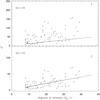 |
Fig. 5 Histogram of χ2 values computed for our entire data set of 73 nights using η = 1.0 (top) and η = 1.5 (bottom). The solid line shows the theoretical χ2 estimator at p = 0.5 for various degrees of freedom (see Sect. 4.2). |
3.2. Data reduction
All pre-processing of the images (bias subtraction, flat-fielding and cosmic-ray removal) was done by applying standard procedures in the IRAF3 and MIDAS4 software packages. The instrumental magnitudes of the target AGN (quasars) and the stars in the image frames were determined by aperture photometry, using DAOPHOT II5 (Stetson 1987). The magnitude of the target AGN was measured relative to the nearby apparently steady comparison stars present on the same CCD frame (Table 2). In this way Differential Light Curves (DLCs) of each AGN were derived relative to 3 comparison stars designated as S1, S2, S3. These comparison stars are within about a magnitude of the target AGN, this precaution being important for minimizing the possibility of spurious INOV detection (e.g., Cellone et al. 2007). In our study the B−R colours of quasars and the comparison stars are often quite different (Table 2). However it is shown by Carini et al. (1992) and Stalin et al. (2004a) that such colour differences do not yield a significant amount of spurious INOV due to the different second-order extinction coefficients of the quasar and the comparison stars as they are observed through varying airmass during the course of monitoring. For the airmass range between 1 and 2 the B−R colour difference between the quasar and the comparison star as high as 1.9 causes negligible errors.
For each night, an optimum aperture radius for photometry was selected on the basis of the observed dispersions in the star-star DLCs that were found for different aperture radii starting from the median seeing (FWHM) value on that night to 4 times that value. We selected the appropriate aperture for each night as the one that provided the minimum dispersion for the steadiest DLC found among all pairs of the comparison stars (e.g., Stalin et al. 2004a). Typically, the selected aperture radius was ~4′′ and the seeing was found to be ~2′′.
4. Results
4.1. Differential Light Curves (DLCs)
The intranight DLCs for the LPCDQs and HPCDQs observed in our monitoring programme are shown in Figs. 1 and 2 respectively, while the corresponding DLCs showing their long-term optical variability (LTOV) are displayed in Figs. 3 and 4. Tables 3 and 4 summarize the results of the INOV observations of our sets of LPCDQs and HPCDQs made by us and augmented with those taken from the literature (Sect. 2).
4.2. Estimation of the parameter η
It has been found in several published studies that the photometric errors returned by the APPHOT6 package are systematically too low such that the rms error for each datapoint is underestimated by a factor η, found to range between 1.30 and 1.75 (Gopal-Krishna et al. 1995; Garcia et al. 1999; Stalin et al. 2004a; Bachev et al. 2005). To verify and quantify this factor for the present set of observations and the version of the APPHOT used here, we have made a fresh estimate of η as follows. Out of the 3 star-star DLCs available for each night (using the 3 comparison stars monitored), we first selected the steadiest star−star DLC. Thus, for our entire dataset (73 nights) we get 73 “steady” DLCs, whose stars appear to have not varied on the corresponding night. For each selected DLC with Np data points, we then computed the χ2 corresponding to its number of degrees of freedom (ν = Np−1). In Fig. 5, we plot for each night, the computed χ2 value together with its corresponding expectation values of χ2 at p = 0.5 which corresponds to 50 per cent probability. It is seen that for most of the “steady” star-star DLCs the calculated χ2 values lie above their expectation values when no correction factor is applied to the photometric errors (i.e, η = 1, top diagram). However, when a correction factor of η = 1.5, is applied to all the data points, the computed χ2 values for the 73 nights are found to be evenly dsitributed about the solid curve showing the expectation values, as is indeed expected for the median estimator of the distribution (bottom diagram). We therefore adopt η = 1.5, for scaling up the IRAF photometric rms errors.
4.3. Peak-to-peak INOV amplitude (ψ)
The peak-to-peak INOV amplitude is calculated using the definition of Romero et al. (1999) 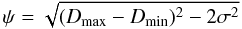 (1)with Dmin,max = minimum (maximum) in the AGN differential light curve, and σ2= η2
 . where, η =1.5.
4.4. INOV detection; F-statistics
Hitherto the criterion most commonly used in the literature for checking the presence of INOV is based on the so-called “C-statistic”, which is defined as the ratio of standard deviations of the “QSO-star” DLC and the corresponding “star-star” DLC (e.g., Jang & Miller 1997; Romero et al. 1999; Stalin et al. 2004, 2005; Xie et al. 2004; Carini et al. 2007; Gupta et al. 2008; Goyal et al. 2010). Recently, de Diego (2010) has emphasized that the usual definition of C is not a proper statistic, as it is based on the ratio of standard deviations which (unlike variance) are not lineal statistical operators. They argue that the critical values for the C-test are wrongly established, being much larger (i.e., more conservative) than those for the F-test which is based on the ratio of variances. In addition, the commonly employed test based on the C-statistic ignores the number of degrees of freedom in the observation, which too is inappropriate. A version of the C-statistic that properly incorporates degrees of freedom can be devised (Villforth et al. 2010), but has not yet been used in INOV studies. Therefore, in this work we shall employ the F-statistics to quantify INOV detection which is defined as follows (Villforth et al. 2010):  (2)where varobserved is the variance of the flux measurements in a DLC and varexpected is the mean of the squares of flux error estimates.
In computing the F-value we first examined the “star-star” DLCs derived from (typically 3) comparison stars monitored along with the quasar in the same session (Figs. 1 and 2), in order to select the steadiest DLC out of them. The corresponding two stars are designated as CS1 and CS2 (they are not necessarily the stars labelled as S1 and S2 in the Figs. 1 and 2), with the convention that CS1 is better matched to the quasar in R-magnitude, compared to CS2. After adjusting for the underestimation of the measurement errors (Sect. 4.2) by setting η = 1.5, F-values can be written as, 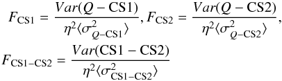 (3)where Var(Q−CS1), Var(Q−CS2) and Var(CS1−CS2) are the variances of the “quasar-CS1”, “quasar-CS2” and “CS1-CS2” DLCs and
  ,
,  and
and  are the mean square (formal) rms errors of the individual data points in the “quasar-CS1”, “quasar-CS2” and “CS1-CS2” DLCs, respectively.
In this way, the F-value was computed for each DLC and compared with the critical F-value,  , where α is the significance level set by us for the test and ν (= Np−1) is the degree of freedom for the DLC. The smaller the value of α, the more unlikely is the variation to occur by chance. For the present study, we have used two significance levels, α = 0.01 and 0.05, corresponding to confidence levels of p > 99 per cent and p > 95 per cent, respectively. Thus, in order to claim a genuine INOV detection, i.e., assigning a designation “variable” designation (V), we stipulate that the computed F-value is above the critical F-value corresponding to p > 0.99. A “possible variable” (PV) designation was assigned when the confidence level for the DLC was found to be in the range 0.95 < p ≤ 0.99, while a “non-variable” (N) designation was assigned if p ≤ 0.95. Tables 3 and 4 summarize the INOV results for our sets of LPCDQs and HPCDQs, both the ones monitored by us and those for which we have taken the DLCs from the literature (Sect. 2). We have carried out the F-test independently for the DLCs of each quasar, drawn relative to CS1 and CS2, yielding two estimates of the INOV duty cycle (Sect. 4.5) for the LPCDQ set and also for the HPCDQ set (Table 5). Good agreement between the two estimates of duty cycle is found, despite the different levels of brightness mismatches of the quasar from the two chosen comparison stars (Tables 3 and 4). This provides a post facto validation of our assumption that the F-test is not unacceptably sensitive to the typical rms errors on individual data points being slightly different for the two DLCs involved in the F-test for each quasar, namely, “Q-CS1” and “Q-CS2”. It needs to be mentioned here that care has been taken that the comparison stars are nearly always within 1-mag of the respective quasars. (For the LPCDQ set, the median magnitude mismatch is 0.3-mag for CS1 and 0.8-mag for CS2 and the corresponsing values for the HPCDQ set are 0.9-mag and 1.4-mag, respectively).
Estimates of DC for our sets of LPCDQs and HPCDQs (using the chosen 2 comparison stars).
It is seen that for a total 11 out of 73 nights, the quasar variability status inferred from the DLC using one comparison star (CS1) differs from that found using the DLC using the other comparison star (CS2). A possible explanation is that one of the stars may have varied. Since such putative low-level INOV of the comparison star would remain unnoticed by eye and hence we have no justification to prefer one comparison star over the other (in terms of steadiness), we list in Table 5 the estimates of INOV duty cycle (DC) for each quasar using both comparison stars, CS1 and CS2 (chosen because their DLC appeared to be the steadiest). While quoting the DC estimates for our sets of LPCDQs and HPCDQs in Sect. 4.5, we take the average of the two estimates of DC arrived at by using CS1 and CS2.
Here it may be recalled that the F-test provides less statistical power (i.e., more non-detections of actually variable sources) than an alternative like the “analysis of variance”, or ANOVA, which tests for differences between the mean values, instead of the contrast between the variances (e.g., de Diego 2010). However, the relatively long exposures required in our measurements means that many of our light curves had fewer than 30 data points, precluding us from applying the ANOVA test with sufficient power.
4.5. The computation of INOV duty cycle (DC)
The INOV duty cycle was computed following the definition of Romero et al. (1999) (see, also, Stalin et al. 2004a): 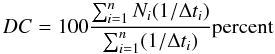 (4)where Δti = Δti,obs(1 + z)-1 is duration of the monitoring session of a source on the ith night, corrected for its cosmological redshift, z. Note that since for a given source the monitoring durations on different nights were not always equal, the computation of DC has been weighted by the actual monitoring duration Δti on the ith night. Ni was set equal to 1 if INOV was detected, otherwise Ni = 0.
Employing the F-statistics the computed INOV DCs are: 28 per cent for LPCDQs (45 per cent if the “PV” cases are included) based on 44 nights’ monitoring (Table 3); and 68 per cent (70 per cent if one “PV” case is included) for the HPCDQs based on 29 nights’ data (Table 4). If only the nights showing ψ > 3 per cent are considered (all of which, clearly, belong to the “V” category), the derived DCs are 7 and 40 per cent for LPCDQs and HPCDQs, respectively.
At p = 0.99, the expected value of false positives for our data sets of LPCDQs (44 nights) and HPCDQs (29 nights) are, 0.44 and 0.29, respectively. Thus, in both cases, we expect no more than ~1 DLC to be falsely classified as variable. Similarly, at p = 0.95, the expected value of false positives for our two data sets of LPCDQs and HPCDQs are < 3 and < 2, respectively.
In order to ensure a consistent analysis and the check on the error estimates, we have also estimated the rate of false positives using actual data, namely our data sets of LPCDQs and HPCDQs. To do this, we have performed the F-test analysis on our set of 73 “steady” star-star DLCs based on the same comparison stars that were used to generate the “quasar-star” DLCs we used for computing the DCs. The results are given in Tables 3 and 4. This also provides the “sanity check” on our error estimation as returned by APPHOT/IRAF. From the LPCDQ data set, 2 out of 44 star-star DLCs are found designated as “clear variable”, while the number for the HPCDQ data set is found to be 1 out of 29 star-star DLCs. The good agreement between the expected and observed rates of false positives for our LPCDQ and HPCDQ data sets validates our analysis procedure.
4.6. Notes on individual sources
Below we give brief comments on the variability characteristics of some of the quasars in our sample.
-
LPCDQ J0741 + 3112: this CDQ was monitored by us on4 nights and was found to vary only on 21Jan. 2006 and 22 Dec. 2006. It showed a very clear,almost sinusoidal light curve withψ = 4.9 per cent. Seeing remained stable at 2′′ throughout the monitoring period (bottom panel; Fig. 1).
-
LPCDQ J1229 + 0203: known to be harbouring a mini-blazar (e.g., Impey et al. 1989), this well known CDQ, 3C 273, showed INOV on 2 out of the 3 nights it was monitored by us (Fig. 1).
-
LPCDQ J1357 + 1919: this CDQ has been extensively monitored in our programme on a total of 8 nights. On 28 Mar. 2006, it showed a striking INOV pattern, clearly fading by ~2 per cent during the first 2 h of the monitoring, followed by a steady level for the next 1.5 h and finally a brightening by ~2 per cent in the final 1.5 h (Fig. 1).
-
HPCDQ J0238 + 1637: this CDQ has been known for its nearly 100 per cent INOV duty cycle (e.g., Gopal-Krishna et al. 2011), the present data conform to this (Fig. 2). In addition to our single night’s observations, this CDQ had earlier been monitored in R-band by Sagar et al. (2004) on 3 nights, and on each occasion INOV was confirmed, with ψ ranging between 5 to 20 per cent (Table 4). Likewise, Romero et al. (2002) found it to vary on each night they monitored it, with ψ in the range 7–44 per cent (Table 4).
-
HPCDQ J1159 + 2914: this CDQ is an OVV quasar (Sitko et al. 1985). We monitored it on 3 consecutive nights and it showed INOV on each night, with ψ exceeding about 5, 9 and 16 per cent (Table 4; Fig. 2). Although the mean brightness of the CDQ remained unchanged between the first 2 nights (i.e., 31 Mar. 2012 and 01 Apr. 2012) later it showed strong inter night variability as it brightened by ~0.5 mag between 01 Apr. 2012 and 02 Apr. 2012.
-
HPCDQ J1256−0547: this famous CDQ, 3C 279, is known to have a high and variable polarization and was the first flat-spectrum quasar to be detected above 100 GeV (Albert et al. 2008). It showed INOV on all the 3 nights we monitored it, with ψ values of 4, 10 and 22 per cent (Table 4; Fig. 2).
5. Discussion and conclusions
In the present study we have made a quantitative comparison of the INOV characteristics of two sets of bright radio core-dominated quasars, both showing strong broad optical emission lines but differring markedly in fractional optical polarization, Pop. To illustrate this we display in Fig. 6 the distributions of Pop and five other basic parameters for our sets of LPCDQs and HPCDQs. The parameters are: redshift (z); blue absolute magnitude, (MB); radio spectral index (αr); radio core-fraction (fc), which is a well known orientation indicator because the extended radio lobe flux density is essentially independent of orientation, while the core flux density is Doppler boosted when the radio source axis is oriented near the line-of-sight (e.g., Kapahi & Saikia 1982; Orr & Browne 1982; Morisawa & Takahara 1987); and luminosity of the extended radio emission (Pext) at 5 GHz, which is a measure of the jet’s intrinsic power (e.g., Willott et al. 1999; Punsly 2005). Application of the two-sample Kolmogorov-Smirnov test shows that the null hypothesis that our sets of LPCDQs and HPCDQ belong to the same parent population cannot be rejected for the parameters z, MB, αr, fc and Pext (Table 6), whereas the hypothesis that they are drawn from the same distribution of Pop, can be rejected at high confidence (>99.9 per cent). Thus, Pop is the key discriminator between our sets of LPCDQs and HPCDQs.
Here it may be relevant to point out that the optical flux of HPCDQs may have a significant, even dominant, synchrotron component contributed by the relativistic jet. In that event, our HPCDQ set would be systematically weaker intrinsically compared to the LPCDQ set, since they are of similar absolute optical magnitudes. Unfortunately, it is not possible at present to quantify and subtract out the jet’s contribution reliably. Nonetheless, even if any such a bias is significant for our datasets, that would probably mean that the central black holes in our LPCDQs are, on average, more massive than those present in our HPCDQ set. Unfortunately, there is at present no knowledge about the dependence of INOV on the mass of the central black hole, although significant information does exist concerning the long-term optical variability (LTOV, on year-like time scales in the rest frame). Using large samples of SDSS quasars it has been found that the quasars containing more massive central black holes tend to exhibit stronger long-term optical variability (Wold et al. 2007; Bauer et al. 2009). Thus, at least on the basis of the observed trend in the quasar LTOV, which correlates positively with both optical polarization (Sect. 1) and central black hole mass, there is little reason to suspect that the stronger INOV found here for the HPCDQ set, in comparison to the LPCDQ set, results from of the latter being optically more luminous and hence probably containing more massive central black holes.
Our choice of F-statistic in the present study (Sect. 4.4) precludes us from making an exact comparison of the present results with those available in the literature (which are mostly based on the C-statistic, Sect. 1). Our main finding is that even though relativistically Doppler boosted (radio) jets are prominent in all 12 LPCDQs, the duty cycle for strong INOV (DC ~ 7 per cent for ψ > 3%) is much smaller than that found for their high polarization counterparts, namely the 9 HPCDQs (DC ~ 40 per cent for ψ > 3%) (Sect. 4.5). Further, the result (Table 4) that INOV amplitudes above 3% are almost exclusively observed for HPCDQs and only rarely seen in LPCDQs (despite their being strongly beamed too), makes HPCDQs closely resemble LBLs in their INOV behaviour (see Gopal-Krishna et al. 2003; 2011; Stalin et al. 2004a,b). The distributions of ψ for our sets of 12 LPCDQs (44 DLCs; Table 3) and 9 HPCDQs (29 DLCs; Table 4) are compared in Fig. 7. It needs to be clarified that the intra night monitoring durations are very similar for these sets of LPCDQ and HPCDQ, the median values being 5.7 and 5.8 h, respectively. Such a matching is desirable in view of the fact that INOV detection probability is at least moderately sensitive to the monitoring duration (e.g., Romero et al. 2002; Carini et al. 2007). A two sample Kolmogorov-Smirnov (K-S) test performed on these ψ distributions rejects the null hypothesis that the two are drawn from the same parent population, giving it a probability of only 3 × 10⁻⁴. This statistical comparison confirms that HPCDQs are much more prone to display INOV than their weakly polarized counterparts, LPCDQs. In stark contrast to the HPCDQ set, ψ was found to exceed 4 per cent level only once out of the 44 nights of LPCDQ monitoring by us. This occurred for the LPCDQ J0741 + 3112 which attained ψ = 4.9 per cent on 21 January 2006 (Table 2). Interestingly, its light-curve on that night showed an extraordinary, almost sinusoidal pattern (Fig. 1), similar to the rare events recorded earlier for the archetypal intra-day variable blazar S5 0716 + 714 on the nights of 1 January 2004 (Wu et al. 2005) and 1 April 2008 (Stalin et al. 2009). We, therefore, consider the LPCDQ J0741 + 3112 to be a good candidate where a transition from LPCDQ to HPCDQ phase might have occured, as reported for the quasar 1633 + 382 (Sect. 1). Hence, optical polarimetric monitoring of J0741 + 3112 would be particularly interesting.
The present observations also provide information on long-term optical variability (LTOV) on month-like or longer timescales (Figs. 3 and 4), we find such variability to be common among both LPCDQs and HPCDQs, with amplitudes approaching 0.1-mag level in the R-band. This result is in accord with the findings of Webb & Malkan (2000) for more common types of AGN; for roughly half the AGNs they found optical variability amplitudes of 0.1–0.2 mag (rms) on month-like time scales. Since the total time span covered in our observations differ vastly from source to source, these data do not permit a quantitative comparison of the LTOV of the HPCDQs and LPCDQs monitored.
In summary, the point emerging from the present study is that for strong INOV, optical polarization is a key requirement even when a strongly beamed synchrotron radio jet is observed (see, Sect. 5). This echoes the well known close connection between the optical polarization of quasars and their long-term optical variability (e.g., Moore & Stockman 1984; Impey et al. 1991). In other words, just as the INOV amplitude and duty cycle for powerful AGNs are not automatically bolstered due to radio loudness, as already inferred in the first part of our programme from the similarities of the INOV levels found for LDQs, LPCDQs and RQQs (see Stalin et al. 2004b, 2005; also, Ramírez et al. 2009; Sect. 1), the present study provides a strong hint that relativistic beaming (as indicated by the radio core dominance) is normally not a sufficient condition for the occurence of strong INOV, unless it is accompanied by a strong optical polarization. Furthermore, this trend exists even if the polarization was measured in relatively distant past (see below).
Thus, even though the polarized optical flux is widely regarded as a manifestation of relativistically beamed nonthermal emission (e.g., Malkan & Moore 1986; Impey et al. 1991), the physical connection of optical polarization to INOV appears to supercede the link between INOV and relativistic beaming. This is evident from the much more modest INOV found for LPCDQs, even though they are core-dominated like the HPCDQs and hence also possess relativistically beamed jets. Now, it is conceivable that the jets are so curved that their inner, optically radiating, beamed segments are misdirected from us (evidence for bending between the sub-parsec and parsec scales does exist for blazars, e.g., Lobanov & Zensus 1999; Readhead et al. 1983). However, this explanation is unlikely to account for the persistent lack of strong INOV among LPCDQs, firstly since jet bending on sub-parsec scale is much milder for LPCDQs (Impey et al. 1991) and, secondly because it is known to vary on month/year-like time scales (e.g., Britzen et al. 2010 and references therein), whereas the optical polarization measurements used for selecting our LPCDQ set were carried out more than a decade ago (Sect. 2). This then suggests that the propensity of a given radio core-dominated quasar to exhibit strong INOV is of a fairly stable nature and it correlates rather tightly with optical polarization class. This inference may appear to run counter to the notion that FSRQs keep switching between high- and low-polarization states (HPCDQ ↔ LPCDQ; Sect. 1), in case the typical time scale for such transitions is much shorter than the decade−like time interval between their optical polarimetric classification and their INOV observations reported here. Conceivably, such polarimetric phase transitions could occur on fairly short, say, year-like time scales that characterise successive ejections of blobs of synchrotron plasma (VLBI knots) out of the central engine (e.g., Aller et al. 2006; Bell & Comeau 2010; Hovatta et al. 2007; León-Taveres et al. 2010; also, Impey & Tapia 1990). However, were this indeed the case, then during the decade long time interval elapsed since the original optical polarimetry, the Pop distribution within the sets of LPCDQs and HPCDQs would have gotten substantially randomized by the time their INOV observations took place. Consequently, little difference should have been found between the INOV duty cycles for the LPCDQ and HPCDQ sets, in clear contradiction to the present result. For a more direct check on this, a fresh round of optical polarimetry is encouraged for the sets of LPCDQs and HPCDQs (which are fairly bright, Table 1), particularly for the two LPCDQs which have exhibited unusually strong INOV (ψ > 3 per cent) during our monitoring (Sect. 4.6).
Recent radio VLBI and optical (and sometimes even X-ray) monitoring observations of a few blazars have provided useful insight into the likely physics behind the flaring and polarization of their emission. According to an emerging picture (e.g., D’Archangelo et al. 2007; Jorstad et al. 2007; Marscher et al. 2008; Arshakian et al. 2010; León-Taveres et al. 2010), much of the polarized optical and radio synchrotron flux and its flaring arise as the successive energetic disturbances emanating from the central engine and then traversing the helical magnetic field along the jet’s initial acceleration/collimation zone, cross through a standing shock in the jet. Such standing shocks typically form at a projected distance of a few parsecs from the central engine, where particle acceleration takes place and the inflowing synchrotron plasma is locally compressed. In this scenario, the magnetic field near the end of the jet’s acceleration zone (which may extend from the central engine up to ~104 times the gravitational radius of the supermassive black hole, e.g., Vlahakis & Königl 2004; Meier & Nakamura 2006) is predominantly longitudinal to the jet, probably due to velocity shear (e.g., Jorstad et al. 2007). However, a build-up of turbulence in this region, e.g., due to weakening of the collimating helical magnetic field (e.g., Arshakian et al. 2010), or some externally induced disturbance (see below), can locally generate a substantial transverse component of magnetic field in the flow. As this turbulent jet plasma passes through the standing shock downstream, not only will particle acceleration and the plasma compression take place, boosting the multi-band synchrotron output, but the same compression would also amplify any transverse component of the pre-shock magnetic field (e.g., caused due to the turbulence, as mentioned above), giving rise to an enhanced polarization signal (e.g., Hughes et al. 1985; Marscher & Gear 1985; Laing 1980). If now the postulated zone of turbulence in the jet, just upstream of the standing shock, is identified as the site where the bulk of INOV arises, then the scenario sketched here may provide a plausible explanation for the close link of INOV to optical polarization underscored in this study. Conversely, if a strong confining helical field persists in LPCDQs, this would tend to subdue the growth of turbulence in the jet plasma, leading to both a weak INOV and a milder build-up of the transverse component of magnetic field in that region. The latter would then result in only a modest field amplification as the jet plasma undergoes compression while crossing the first (transverse) standing shock. An observational constraint which this simple picture must satisfy is that the postulated zone of turbulence upstream of the standing shock in blazar jets must be a fairly long lasting feature, for consistency with the observed persistence of strong INOV we find for HPCDQs vis à vis LPCDQs, even a decade after their optical polarimetry was carried out and the HPCDQ/LPCDQ status defined. Interestingly, such a time scale is much longer than the typical month/year-like intervals observed between the nuclear ejections, as mentioned above.
Detailed characterization of the rapid optical variability has assumed added relevance in the present Fermi-LAT era (Atwood et al. 2009). Recent TeV monitoring has revealed ultra-fast variability on minute-like time scales for a few blazars (Aharonian et al. 2007; Albert et al. 2007; Acciari et al. 2009; Aleksić et al. 2011). A scenario proposed to explain such γ-ray flaring invokes disturbance caused in the jet flow by the passage of red giant stars through the inner jet which is normally opaque to radio emission (Barkov et al. 2012). In this mechanism, continued impact of the jet flow would blow out the extended atmospheres of such intruding stars, forming magnetized condensations accelerated to high bulk Lorentz factors. The concomitant shocks at these condensations would lead to particle accelaration, accounting for the ultra-rapid TeV flux variations. Interestingly, this same process would also excite turbulence in the jet plasma (the process invoked above for the origin of INOV), powered by the red giants and their wakes crossing the jet. With a typical stellar velocity of ≲ 103 km s-1 the expected crossing time of the inner jet by the star is ≳ 102–103 yr and so the postulated enhanced turbulence level in the affected jet sedgement can be a long lasting feature, consistent with the persistence of enhanced INOV in blazars underscored in the present work. However, within this basic scenario it remains to be clearly understood why, unlike the γ-ray flaring, INOV has been so rarely detected on sub-hour time scales (e.g., Gopal-Krishna et al. 2011).
A potentially very useful tool for constraining INOV mechanism in different AGN classes is the observation of intra-night variability of polarized light, though very few systematic studies have been reported. A preliminary investigation by Andruchow, Romero & Cellone (2005) indicated that at least for BL Lac objects, the occurence of optical polarization variability on sub-hour times scales is not so rare, unlike the case for optical continuum variability (e.g., Gopal-Krishna et al. 2011). A more extensive study of polarization INOV (“PINOV”) has been reported by Villforth et al. (2009), who monitored an AGN sample consisting of 12 RQQs, 8 BL Lacs and 8 FSRQs, albeit for only a single session lasting about 4 h per AGN. They concluded that for sources having Pop ≥ 5%, PINOV is ubiquitous but it is less frequent among BL Lacs and FSRQs showing lower Pop. Based on this, they have associated PINOV with instabilities in the jet or changing physical conditions in the jet plasma.
To sum up, the main conclusion emerging from the present work is that compared to HPCDQs the INOV exhibited by LPCDQs is distinctly milder and large-amplitude INOV with ψ > 3 per cent is very rarely seen for them. Given that strong beaming of the nuclear jets is already occuring in both HPCDQs and LPCDQs, it would appear from the present work that the effective ‘switch’ for strong intranight optical variability is the presence of optical polarization, even if its measurement preceded the INOV observations by several years. To effectively probe this point and the connection between INOV and TeV flaring on hour-like or shorter time scales, it is important to carry out more sensitive intranight optical monitoring of flat-spectrum quasars (both HPCDQs and LPCDQs), preferrably in the polarimetric mode and in coordination with their monitoring at TeV energies.
Online material
Positions and magnitudes of the CDQs and the comparison stars∗.
 |
Fig. 1 The intranight optical DLCs of the LPCDQs monitored in the present study. For each night, the source name, the telescope used, the date, and the duration of monitoring are given at the top. The upper 3 panels show the DLCs of the LPCDQ relative to 3 comparison stars while the attached lower 3 panels show the star-star DLCs, where the solid horizontal lines mark the mean for each star-star DLC. The bottom panel gives the plots of seeing variation for the night, based on 3 stars monitored along with the blazar on the same CCD frame. |
 |
Fig. 1 continued. |
 |
Fig. 1 continued. |
 |
Fig. 1 continued. |
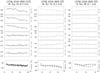 |
Fig. 1 continued. |
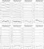 |
Fig. 2 The intranight optical DLCs of the HPCDQ monitored in the present study. For each night, the source name, the telescope used, the date, and the duration of monitoring are given at the top. The upper 3 panels show the DLCs of the HPCDQ relative to 3 comparison stars while the attached lower 3 panels show the star-star DLCs, where the solid horizontal lines mark the mean for each star-star DLC. The bottom panel gives the plots of seeing variation for the night, based on 3 stars monitored along with the blazar on the same CCD frame. |
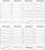 |
Fig. 2 continued. |
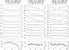 |
Fig. 2 continued. |
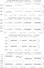 |
Fig. 3 Long-term optical variability (LTOV) DLCs for the LPCDQs monitored in the present study; source name and the total time span covered are at the top of each panel. |
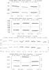 |
Fig. 3 continued. |
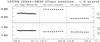 |
Fig. 3 continued. |
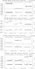 |
Fig. 4 As in Fig. 3 for the HPCDQs monitored in the present study. |
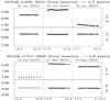 |
Fig. 4 continued. |
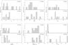 |
Fig. 6 Distributions of z, MB, αr, fc, Pext and Pop for our two sets of CDQs: LPCDQs (upper panels; vertical stripes); HPCDQs (lower panels; horizontal stripes) (Sect. 5; Table 1). |
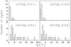 |
Fig. 7 Distribution of INOV amplitude (ψ), for LPCDQs (upper panel; vertical stripes) and HPCDQs (lower panel; horizontal stripes), estimated from the DLCs drawn using the two comparison stars, CS1 and CS2. |
Image reduction and analysis facility (http://iraf.noao.edu/)
Munich image and data analysis system http://www.eso.org/sci/data-processing/software/esomidas//
Dominion astrophysical observatory photometry software.
Photometry package in IRAF.
Acknowledgments
The authors thank Dr. Vijay Mohan for help during the observations at IGO and Dr. C.S. Stalin for making available his quasar optical monitoring data in digital form. The authors wish to acknowledge the support received from the staff of the IAO and CREST of IIA and IGO. We are very thankful to an anonymous referee for carefully reviewing the manuscript and for making several constructive suggestions. This research has made use of NASA/IPAC Extragalactic Database (NED), which is operated by the Jet Propulsion Laboratory, California Institute of Technology, under contract with National Aeronautics and Space Administration.
References
- Acciari, V. A., Aliu, E., Arlen, T., et al. 2009, Science, 325, 444 [NASA ADS] [CrossRef] [PubMed] [Google Scholar]
- Aharonian, F., Akhperjanian, A. G., Bazer-Bachi, A. R., et al. 2007, ApJ, 664, L71 [Google Scholar]
- Albert, J., Aliu, E., Anderhub, H., et al. 2007, ApJ, 669, 862 [NASA ADS] [CrossRef] [Google Scholar]
- Albert, J., Aliu, E., Anderhub, H., et al. (MAGIC Collaboration) 2008, Science, 320, 1752 [NASA ADS] [CrossRef] [PubMed] [Google Scholar]
- Aleksić, J., Antonelli, L. A., Antoranz, P., et al. 2011, ApJ, 730, L8 [NASA ADS] [CrossRef] [Google Scholar]
- Algaba, J. C., Gabuzda, D. C., & Smith, P. S. 2011, MNRAS, 411, 85 [NASA ADS] [CrossRef] [Google Scholar]
- Aller, M. F., Aller, H. D., & Hughes, P. E. 2003, ApJ, 586, 33 [NASA ADS] [CrossRef] [Google Scholar]
- Aller, M. F., Aller, H. D., & Hughes, P. E. 2006, in Blazar Variability Workshop II: Entering the GLAST Era, eds. H. R. Miller, K. Marshall, J. R. Webb, & M. F. Aller (San Francisco: ASP), ASP Conf. Ser., 350, 25 [Google Scholar]
- Andruchow, I., Romero, G. E., & Cellone, S. A. 2005, A&A, 442, 97 [NASA ADS] [CrossRef] [EDP Sciences] [Google Scholar]
- Angel, J. R. P., & Stockman, H. S. 1980, ARA&A, 321, 61 [Google Scholar]
- Antonucci, R. R. J., & Ulvestad, J. S. 1985, ApJ, 294, 158 [NASA ADS] [CrossRef] [Google Scholar]
- Arshakian, T. G., León-Tavares, J., Lobanov, A. P., et al. 2010, MNRAS, 401, 1231 [NASA ADS] [CrossRef] [Google Scholar]
- Atwood, W. B., Abdo, A. A., Ackermann, M., et al. 2009, ApJ, 697, 1071 [NASA ADS] [CrossRef] [Google Scholar]
- Bai, J. M., & Lee, M. G. 2005, JKAS, 38, 125 [NASA ADS] [CrossRef] [Google Scholar]
- Bardelli, S., Zucca, E., Bolzonella, M., et al. 2009, A&A, 495, 431 [NASA ADS] [CrossRef] [EDP Sciences] [Google Scholar]
- Barkov, M. V., Aharonian, F. A., Bogovalov, S. V., Kelner, S. R., & Khangulyan, D. 2012, ApJ, 749, 119 [NASA ADS] [CrossRef] [Google Scholar]
- Bauer, A., Baltay, C., Coppi, P., et al. 2009, ApJ, 696, 1241 [NASA ADS] [CrossRef] [Google Scholar]
- Becker, P. A., Das, S., & Le, T. 2008, ApJL, 677, 93 [Google Scholar]
- Bell, M. B., & Comeau, S. P. 2010, Ap&SS, 325, 31 [NASA ADS] [CrossRef] [Google Scholar]
- Berriman, G., Schmidt, G. D., West, S. C., & Stockman, H. S. 1990, ApJS, 74, 869 [NASA ADS] [CrossRef] [Google Scholar]
- Blundell, K. M., & Kuncic, Z. 2007, ApJ, 668, L103 [NASA ADS] [CrossRef] [Google Scholar]
- Briggs, F. H. 1983, ApJ, 88, 239 [Google Scholar]
- Britzen, S., Witzel, A., Gong, B. P., et al. 2010, A&A, 515, 105 [Google Scholar]
- Carini, M. T. 1990, Ph.D. Thesis, George State University [Google Scholar]
- Carini, M. T., Miller, H. R., & Goodrich, B. D. 1990, AJ, 100, 347 [NASA ADS] [CrossRef] [Google Scholar]
- Carini, M. T., Miller, H. R., Noble, J. C., & Goodrich, B. D. 1992, AJ, 104, 15 [NASA ADS] [CrossRef] [Google Scholar]
- Carini, M. T., Noble, J. C., Taylor, R., & Culler, R. 2007, AJ, 133, 303 [NASA ADS] [CrossRef] [Google Scholar]
- Cao, X. 2003, ApJ, 599, 147 [NASA ADS] [CrossRef] [Google Scholar]
- Cellone, S. A., Romero, G. E., & Combi, J. A. 2000, AJ, 119, 1534 [NASA ADS] [CrossRef] [Google Scholar]
- Cellone, S. A., Romero, G. E., & Araudo, A. T. 2007, MNRAS, 374, 357 [NASA ADS] [CrossRef] [Google Scholar]
- Chand, H., Wiita, P. J., & Gupta, A. C. 2010, MNRAS, 402, 1059 [NASA ADS] [CrossRef] [Google Scholar]
- Czerny, B., Siemiginowska, A., Janiuk, A., & Gupta, A. C. 2008, MNRAS, 386, 1157 [NASA ADS] [CrossRef] [Google Scholar]
- D’Arcangelo, F. D., Marscher, A. P., Jorstad, S. G., et al. 2007, ApJ, 659, L107 [NASA ADS] [CrossRef] [Google Scholar]
- de Diego, J. A. 2010, AJ, 139, 1269 [NASA ADS] [CrossRef] [Google Scholar]
- Drinkwater, M. J., Webster, R. L., Francis, P. J., et al. 1997, MNRAS, 284, 85 [NASA ADS] [Google Scholar]
- Edelson, R., Turner, T. J., Pounds, K., et al. 2002, ApJ, 568, 610 [NASA ADS] [CrossRef] [Google Scholar]
- Fan, J. H. 2005, ChJAA, 5, 213 [NASA ADS] [Google Scholar]
- Fan, J. H., Cheng, K. S., Zhang, L., & Liu, C. H. 1997, A&A, 327, 947 [NASA ADS] [Google Scholar]
- Fan, J. H., & Zhang, J. S. 2003, A&A, 407, 899 [NASA ADS] [CrossRef] [EDP Sciences] [Google Scholar]
- Fomalont, E. B., Frey, S., Paragi, Z., et al. 2000, ApJS, 131, 95 [NASA ADS] [CrossRef] [Google Scholar]
- Francis, P. J., Whiting, M. T., & Webster, R. L. 2000, PASA, 17, 56 [NASA ADS] [CrossRef] [Google Scholar]
- Fugmann, W. 1988, A&A, 205, 86 [NASA ADS] [Google Scholar]
- Gabuzda, D. C., & Cawthorne, T. V. 1996a, MNRAS, 283, 759 [NASA ADS] [CrossRef] [Google Scholar]
- Gabuzda, D. C., Sitko, M. L., & Smith, P. S. 1996b, AJ, 112, 1877 [NASA ADS] [CrossRef] [Google Scholar]
- Garcia, A., Sodré, L., Jablonski, F. J., & Terlevich, R. J. 1999, MNRAS, 309, 803 [NASA ADS] [CrossRef] [Google Scholar]
- Gaskell, C. M. 2008, Rev. Max. Astron. Astrofis., 32, 1 [Google Scholar]
- Ghisellini, G., & Celloti, A. 2001, A&A, 379, L1 [NASA ADS] [CrossRef] [EDP Sciences] [Google Scholar]
- Giommi, P., Padovani, P., Polenta, G., et al. 2012, MNRAS, 420, 2899 [NASA ADS] [CrossRef] [Google Scholar]
- Gopal-Krishna, Sagar, R., & Wiita, P. J. 1995, MNRAS, 274, 701 [NASA ADS] [CrossRef] [Google Scholar]
- Gopal-Krishna, Stalin, C. S., Sagar, R., & Wiita, P. J. 2003, ApJ, 586, L25 [NASA ADS] [CrossRef] [Google Scholar]
- Gopal-Krishna, Goyal, A., Joshi, S., Karthick, C., et al. 2011, MNRAS, 416, 101 [NASA ADS] [Google Scholar]
- Goyal, A., Gopal-Krishna, J. S., Sagar, R., et al. 2010, MNRAS, 401, 2622 [NASA ADS] [CrossRef] [Google Scholar]
- Gupta, A. C., & Joshi, U. C. 2005, A&A, 440, 855 [NASA ADS] [CrossRef] [EDP Sciences] [Google Scholar]
- Gupta, A. C., Fan, J. H., Bai, J. M., & Wagner, S. J. 2008, AJ, 135, 1384 [NASA ADS] [CrossRef] [Google Scholar]
- Helmboldt, J. F., Taylor, G. B., Tremblay, S., et al. 2007, ApJ, 658, 203 [NASA ADS] [CrossRef] [Google Scholar]
- Hovatta, T., Tornikoski, M., Lainela, M., et al. 2007, A&A, 469, 899 [NASA ADS] [CrossRef] [EDP Sciences] [Google Scholar]
- Howard, E. S., Webb, J. R., Pollock, J. T., & Stencel, R. E. 2004, AJ, 127, 17 [NASA ADS] [CrossRef] [Google Scholar]
- Hughes, P. A., Aller, H. D., & Aller, M. F. 1985, ApJ, 298, 301 [NASA ADS] [CrossRef] [Google Scholar]
- Impey, C. D., & Tapia, S. 1990, ApJ, 354, 124 [NASA ADS] [CrossRef] [Google Scholar]
- Impey, C. D., Malkan, M. A., & Tapia, S. 1989, ApJ, 347, 96 [NASA ADS] [CrossRef] [Google Scholar]
- Impey, C. D., Lawrence, C. R., & Tapia, S. 1991, ApJ, 375, 46 [NASA ADS] [CrossRef] [Google Scholar]
- Jang, M., & Miller, H. R. 1995, ApJ, 452, 582 [NASA ADS] [CrossRef] [Google Scholar]
- Jannuzi, B. T., Smith, P. S., & Elston, R. 1993, ApJS, 85, 265 [NASA ADS] [CrossRef] [Google Scholar]
- Jorstad, S. G., Marscher, A. P., Stevens, J. A., et al. 2007, AJ, 134, 799 [NASA ADS] [CrossRef] [Google Scholar]
- Kapahi, V. K., & Saikia, D. J. 1982, JApA, 3, 465 [NASA ADS] [CrossRef] [Google Scholar]
- Koratkar, A., Antonucci, R., Goodrich, R., & Storrs, A. 1998, ApJ, 503, 599 [NASA ADS] [CrossRef] [Google Scholar]
- Kovalev, Y. Y., Nizhelsky, N. A., Kovalev, Y. A., et al. 1999, A&AS, 139, 545 [NASA ADS] [CrossRef] [EDP Sciences] [Google Scholar]
- Kühr, H., & Schmidt, G. D. 1990, AJ, 99, 1 [NASA ADS] [CrossRef] [Google Scholar]
- Laing, R. A. 1980, MNRAS, 193, 439 [NASA ADS] [Google Scholar]
- León-Taveres, J., Lobanov, A. P., Chavushyan, V. H., et al. 2010, ApJ, 715, L355 [NASA ADS] [CrossRef] [Google Scholar]
- Linford, J. D., Taylor, G. B., Romani, R. W., et al. 2011, ApJ, 726, 16 [NASA ADS] [CrossRef] [Google Scholar]
- Lister, M. L., & Smith, P. S. 2000, ApJ, 541, 66 [NASA ADS] [CrossRef] [Google Scholar]
- Lister, M. L., & Homan, D. C. 2005, AJ, 130, 1389 [NASA ADS] [CrossRef] [Google Scholar]
- Lobanov, A. P., & Zensus, J. A. 1999, ApJ, 521, 509 [NASA ADS] [CrossRef] [Google Scholar]
- Malkan, M. A., & Moore, R. L. 1986, ApJ, 300, 216 [NASA ADS] [CrossRef] [Google Scholar]
- Maraschi, L., & Tavecchio, F. 2003, ApJ, 593, 667 [NASA ADS] [CrossRef] [Google Scholar]
- Marscher, A. P., & Gear, W. K. 1985, ApJ, 298, 114 [NASA ADS] [CrossRef] [Google Scholar]
- Marscher, A. P., Jorstad, S. G., D’Arcangelo, F. D., et al. 2008, Nature, 452, 966 [NASA ADS] [CrossRef] [PubMed] [Google Scholar]
- Meier, D. L. 1999, ApJ, 552, 753 [NASA ADS] [CrossRef] [Google Scholar]
- Meier, D. L., & Nakamura, M. 1996, in Blazar Variability Workshop II: Entering the GLAST Era, eds. H. R. Miller, K. Marshall, J. R. Webb, & M. F. Aller (San Francisco: ASP), ASP Conf. Ser., 350, 195 [Google Scholar]
- Meyer, E. T., Fossati, G., Georganopoulos, M., & Lister, M. L. 2011, ApJ, 740, 98 [NASA ADS] [CrossRef] [Google Scholar]
- Mihov, B., Bachev, R., Slacheva-Mihova, L., et al. 2008, AN, 329, 77 [NASA ADS] [Google Scholar]
- Miller, H. R., Carini, M., & Goodrich, B. 1989, Nature, 337, 627 [NASA ADS] [CrossRef] [Google Scholar]
- Monet, D. G., Levine, S. E., Canzian, B., et al. 2003, AJ, 125, 984 [NASA ADS] [CrossRef] [Google Scholar]
- Moore, R. L., & Stockman, H. S. 1981, ApJ, 243, 60 [NASA ADS] [CrossRef] [Google Scholar]
- Moore, R. L., & Stockman, H. S. 1984, ApJ, 279, 465 [NASA ADS] [CrossRef] [Google Scholar]
- Morisawa, K., & Takahara, F. 1987, MNRAS, 228, 745 [NASA ADS] [Google Scholar]
- Nartallo, R., Gear, W. K., Murray, A. G., Robson, E. I., & Hough, J. H. 1998, MNRAS, 297, 667 [NASA ADS] [CrossRef] [Google Scholar]
- Nipoti, C., Blundell, K. M., & Binny, J. 2005, MNRAS, 361, 633 [NASA ADS] [CrossRef] [Google Scholar]
- O’Dea, C. P. 1998, PASP, 110, 747 [NASA ADS] [CrossRef] [Google Scholar]
- Orienti, M., Dallacasa, D., Tinti, S., & Stanghellini, C. 2006, A&A, 450, 9590 [NASA ADS] [CrossRef] [EDP Sciences] [Google Scholar]
- Orr, M. J. L., & Browne, I. W. A. 1982, MNRAS, 200, 1067 [NASA ADS] [CrossRef] [Google Scholar]
- Osterman Meyer, A., Miller, H. R., Marshall, K., et al. 2009, AJ, 138, 1902 [NASA ADS] [CrossRef] [Google Scholar]
- Perlman, E. S., et al. 2008, in Extragalactic Jets: Theory and Observation from Radio to Gamma Ray, eds. T. A. Rector, & D. S. De Young (San Francisco: ASP), ASP Conf. Ser., 386, 147 [Google Scholar]
- Punsly, B. 2005, ApJ, 623, 9 [Google Scholar]
- Ramírez, A., de Diego, J. A., Dultzin, D., & González-Pérez, J.-N., 2009, AJ, 138, 991 [NASA ADS] [CrossRef] [Google Scholar]
- Rani, B., et al. 2010, MNRAS, 404, 1992 [NASA ADS] [Google Scholar]
- Readhead, A. C. S., Hough, D. H., Ewing, M. S., Walker, R. C., & Romney, J. D. 1983, ApJ, 265, 107 [NASA ADS] [CrossRef] [Google Scholar]
- Romero, G. E., Cellone, S. A., & Combi, J. A. 1999, A&AS, 135, 477 [NASA ADS] [CrossRef] [EDP Sciences] [Google Scholar]
- Romero, G. E., Cellone, S. A., Combi, J. A., & Andruchow, I. 2002, A&A, 135, 477 [Google Scholar]
- Sagar, R. 1999, Curr. Sci, 77, 643 [Google Scholar]
- Sagar, R., Stalin, C. S., & Gopal-Krishna, W. P. J. 2004, MNRAS, 348, 176 [NASA ADS] [CrossRef] [Google Scholar]
- Savolainen, T., Wiik, K., Valtaoja, E., Jorstad, S. G., & Marscher, A. P. 2002, A&A, 392, 851 [NASA ADS] [CrossRef] [EDP Sciences] [Google Scholar]
- Scarpa, R., & Falomo, R. 1997, A&A, 325, 109 [NASA ADS] [Google Scholar]
- Schlegel, D. J., Finkbeiner, D. P., & Davis, M. 1998, ApJ, 500, 525 [NASA ADS] [CrossRef] [Google Scholar]
- Schmidt, G. D., & Smith, P. S. 2000, ApJ, 545, 117 [NASA ADS] [CrossRef] [Google Scholar]
- Sitko, M. L., Schmidt, G. D., & Stein, W. A. 1985, ApJS, 59, 323 [NASA ADS] [CrossRef] [Google Scholar]
- Smith, P. S., Williams, G. G., Schmidt, G. D., Diamond-Stanic, A. M., & Means, D. L. 2007, ApJ, 663, 118 [NASA ADS] [CrossRef] [Google Scholar]
- Stalin, C. S., Gopal-Krishna, Sagar, R., & Wiita, P. J. 2004a, JApA, 25, 1 [Google Scholar]
- Stalin, C. S., Gopal-Krishna, Sagar, R., & Wiita, P. J. 2004b, MNRAS, 350, 175 [NASA ADS] [CrossRef] [Google Scholar]
- Stalin, C. S., Gupta, A. C., Gopal-Krishna, W. P. J., & Sagar, R. 2005, MNRAS, 356, 607 [NASA ADS] [CrossRef] [Google Scholar]
- Stalin, C. S., Kawabata, K. S., Uemura, M., et al. 2009, MNRAS, 399, 1357 [NASA ADS] [CrossRef] [Google Scholar]
- Stanghellini, C. 2003, PASA, 20, 118 [NASA ADS] [Google Scholar]
- Stanghellini, C., O’Dea, C. P., Baum, S. A., et al. 1997, A&A, 325, 943 [NASA ADS] [Google Scholar]
- Stetson, P. B. 1987, PASP, 99, 191 [NASA ADS] [CrossRef] [Google Scholar]
- Stocke, J. T., Morris, S. L., Weymann, R. J., & Foltz, C. B. 1992, ApJ, 396, 487 [NASA ADS] [CrossRef] [Google Scholar]
- Stockman, H. S., & Angel, J. R. P. 1978, ApJ, 220, 67 [NASA ADS] [CrossRef] [Google Scholar]
- Stockman, H. S., Moore, R. L., & Angel, J. R. P. 1984, ApJ, 279, 485 [NASA ADS] [CrossRef] [Google Scholar]
- Sun, W.-H., & Malkan, M. A. 1989, ApJ, 346, 68 [NASA ADS] [CrossRef] [Google Scholar]
- Tinti, S., Dallacasa, D., De Zotti, G., Celotti, A., & Stanghellini, A. 2005, A&A, 432, 31 [NASA ADS] [CrossRef] [EDP Sciences] [Google Scholar]
- Torniainen, I., Tornikoski, M., Teräsranta, H., Aller, M. F., & Aller, H. D. 2005, A&A, 435, 839 [NASA ADS] [CrossRef] [EDP Sciences] [Google Scholar]
- Véron-Cetty, M.-P., & Véron, P. 1996, ESO Scientific Report, Garching: European Southern Observatory (ESO), 7th edn. [Google Scholar]
- Véron-Cetty, M.-P., & Véron, P. 2006, A&A, 455, 773 [NASA ADS] [CrossRef] [EDP Sciences] [Google Scholar]
- Villforth, C., Nilsson, K., Ostensen, R., et al. 2009, MNRAS, 397, 1893 [NASA ADS] [CrossRef] [Google Scholar]
- Villforth, C., Koekemoer, A. M., & Grogin, N. A. 2010, ApJ, 723, 737 [NASA ADS] [CrossRef] [Google Scholar]
- Visvanathan, N., & Wills, B. J. 1998, AJ, 116, 2119 [NASA ADS] [CrossRef] [Google Scholar]
- Vlahakis, N., & Königl, A. 2004, in AGN Physics with Sloan Digital Sky Survey, eds. G. T. Richards, & P. B. Hall (San Francisco: ASP), ASP Conf. Ser., 386, 147 [Google Scholar]
- Webb, W., & Malkan, M. 2000, ApJ, 540, 652 [NASA ADS] [CrossRef] [Google Scholar]
- Wagner, S. J., & Witzel, A. 1996, ARA&A, 33, 163 [Google Scholar]
- Wehrle, A. E., Morabito, D. D., & Preston, R. A. 1984, ApJ, 89, 336 [NASA ADS] [CrossRef] [Google Scholar]
- Wills, B. J. 1989, in BL Lac objects, Proceedings of a Workshop Held in Como, Italy, eds. L. Maraschi, T. Maccacaro, & M.-H. Ulrich, 334, 109 [Google Scholar]
- Wills, B. J., Wills, D., Breger, M., Antonucci, R. R. J., & Barvianis, R. 1992, ApJ, 398, 454 [NASA ADS] [CrossRef] [Google Scholar]
- Wiita, P. J. 2006, in Blazar Variability Workshop II: Entering the GLAST Era, eds. H. R. Miller, K. Marshall, J. R. Webb, & M. F. Aller (San Francisco: ASP), ASP Conf. Ser., 350, 183 [Google Scholar]
- Willott, C. J., Rawlings, S., Blundell, K. M., & Lacy, M. 1999, MNRAS, 309, 101 [Google Scholar]
- Wold, M., Brotherton, M. S., & Shang, Z. 1999, MNRAS, 375, 989 [Google Scholar]
- Wu, J., Peng, B., Zhou, X., et al. 2005, A&A, 129, 181 [Google Scholar]
- Wu, Q., Xu, Y-A., & Cao, X. 2011, JApA, 32, 223 [NASA ADS] [CrossRef] [Google Scholar]
- Xie, G. Z., Zhou, S. B., Li, K. H., et al. 2004, MNRAS, 348, 341 [Google Scholar]
All Tables
Estimates of DC for our sets of LPCDQs and HPCDQs (using the chosen 2 comparison stars).
All Figures
|
Fig. 5 Histogram of χ2 values computed for our entire data set of 73 nights using η = 1.0 (top) and η = 1.5 (bottom). The solid line shows the theoretical χ2 estimator at p = 0.5 for various degrees of freedom (see Sect. 4.2). |
| In the text | |
|
Fig. 1 The intranight optical DLCs of the LPCDQs monitored in the present study. For each night, the source name, the telescope used, the date, and the duration of monitoring are given at the top. The upper 3 panels show the DLCs of the LPCDQ relative to 3 comparison stars while the attached lower 3 panels show the star-star DLCs, where the solid horizontal lines mark the mean for each star-star DLC. The bottom panel gives the plots of seeing variation for the night, based on 3 stars monitored along with the blazar on the same CCD frame. |
| In the text | |
|
Fig. 1 continued. |
| In the text | |
|
Fig. 1 continued. |
| In the text | |
|
Fig. 1 continued. |
| In the text | |
|
Fig. 1 continued. |
| In the text | |
|
Fig. 2 The intranight optical DLCs of the HPCDQ monitored in the present study. For each night, the source name, the telescope used, the date, and the duration of monitoring are given at the top. The upper 3 panels show the DLCs of the HPCDQ relative to 3 comparison stars while the attached lower 3 panels show the star-star DLCs, where the solid horizontal lines mark the mean for each star-star DLC. The bottom panel gives the plots of seeing variation for the night, based on 3 stars monitored along with the blazar on the same CCD frame. |
| In the text | |
|
Fig. 2 continued. |
| In the text | |
|
Fig. 2 continued. |
| In the text | |
|
Fig. 3 Long-term optical variability (LTOV) DLCs for the LPCDQs monitored in the present study; source name and the total time span covered are at the top of each panel. |
| In the text | |
|
Fig. 3 continued. |
| In the text | |
|
Fig. 3 continued. |
| In the text | |
|
Fig. 4 As in Fig. 3 for the HPCDQs monitored in the present study. |
| In the text | |
|
Fig. 4 continued. |
| In the text | |
|
Fig. 6 Distributions of z, MB, αr, fc, Pext and Pop for our two sets of CDQs: LPCDQs (upper panels; vertical stripes); HPCDQs (lower panels; horizontal stripes) (Sect. 5; Table 1). |
| In the text | |
|
Fig. 7 Distribution of INOV amplitude (ψ), for LPCDQs (upper panel; vertical stripes) and HPCDQs (lower panel; horizontal stripes), estimated from the DLCs drawn using the two comparison stars, CS1 and CS2. |
| In the text | |
Current usage metrics show cumulative count of Article Views (full-text article views including HTML views, PDF and ePub downloads, according to the available data) and Abstracts Views on Vision4Press platform.
Data correspond to usage on the plateform after 2015. The current usage metrics is available 48-96 hours after online publication and is updated daily on week days.
Initial download of the metrics may take a while.