| Issue |
A&A
Volume 543, July 2012
|
|
|---|---|---|
| Article Number | A120 | |
| Number of page(s) | 8 | |
| Section | Stellar structure and evolution | |
| DOI | https://doi.org/10.1051/0004-6361/201219253 | |
| Published online | 09 July 2012 | |
Amplitudes of solar-like oscillations in red giant stars
Evidence for non-adiabatic effects using CoRoT observations
1 LESIA, CNRS UMR 8109, Observatoire de Paris, Université Pierre et Marie Curie, Université Denis Diderot, Place Jules Janssen, 92195 Meudon Cedex, France
e-mail: This email address is being protected from spambots. You need JavaScript enabled to view it.
2 Institut d’Astrophysique et de Géophysique de l’Université de Liège, Allée du 6 Août 17, 4000 Liège, Belgium
3 Zentrum für Astronomie der Universität Heidelberg, Landessternwarte, Königstuhl 12, 69117 Heidelberg, Germany
4 GEPI, CNRS, Observatoire de Paris, Université Denis Diderot, Place Jules Janssen, 92195 Meudon Cedex, France
5 Institut d’Astrophysique Spatiale, CNRS, Université Paris XI, 91405 Orsay Cedex, France
Received: 21 March 2012
Accepted: 18 May 2012
Abstract
Context. A growing number of solar-like oscillations has been detected in red giant stars thanks to the CoRoT and Kepler space-crafts. In the same way as for main-sequence stars, mode driving is attributed to turbulent convection in the uppermost convective layers of those stars.
Aims. The seismic data gathered by CoRoT on red giant stars allow us to test the mode driving theory in physical conditions different from main-sequence stars.
Methods. Using a set of 3D hydrodynamical models representative of the upper layers of sub- and red giant stars, we computed the acoustic mode energy supply rate ( ). Assuming adiabatic pulsations and using global stellar models that assume that the surface stratification comes from the 3D hydrodynamical models, we computed the mode amplitude in terms of surface velocity. This was converted into intensity fluctuations using either a simplified adiabatic scaling relation or a non-adiabatic one.
Results. From L and M (the luminosity and mass), the energy supply rate is found to scale as (L/M)2.6 for both main-sequence and red giant stars, extending previous results. The theoretical amplitudes in velocity under-estimate the Doppler velocity measurements obtained so far from the ground for red giant stars by about 30%. In terms of intensity, the theoretical scaling law based on the adiabatic intensity-velocity scaling relation results in an under-estimation by a factor of about 2.5 with respect to the CoRoT seismic measurements. On the other hand, using the non-adiabatic intensity-velocity relation significantly reduces the discrepancy with the CoRoT data. The theoretical amplitudes remain 40% below, however, the CoRoT measurements.
Conclusions. Our results show that scaling relations of mode amplitudes cannot be simply extended from main-sequence to red giant stars in terms of intensity on the basis of adiabatic relations because non-adiabatic effects for red giant stars are important and cannot be neglected. We discuss possible reasons for the remaining differences.
Key words: stars: solar-type / stars: oscillations / sun: oscillations / turbulence / convection / waves
© ESO, 2012
1. Introduction
Before CoRoT (launched in December 2006), solar-like oscillations had been detected for a dozen of bright red giant stars either from the ground or from space with MOST (e.g., Barban et al. 2007). Thanks to CoRoT and Kepler, it is now possible to detect and measure solar-like oscillations in many more (several thousands) red giant stars (e.g., de Ridder et al. 2009; Huber et al. 2010; Bedding et al. 2010; Kallinger et al. 2010; Stello et al. 2011; Mosser et al. 2012). With such a large set of stars, it is possible to perform ensemble asteroseismology by deriving scaling relations that relate seismic parameters to a few fundamental stellar parameters (e.g. masses, radii, luminosities etc.). These approaches are now commonly applied to global seismic parameters, such as the cutoff-frequency or peak frequency (e.g., Miglio et al. 2009; Stello et al. 2009; Kallinger et al. 2010; Mosser et al. 2010). However, scaling relation is used only infrequently for mode amplitudes. The main reason for this is our poor theoretical understanding of the underlying physical mechanisms for mode driving and damping.
Using a large set of red giant stars observed by CoRoT, Baudin et al. (2011) have derived scaling relations in terms of mode lifetimes and amplitudes. These authors have found that the scaling relation proposed by Samadi et al. (2007) for the mode amplitude significantly departs from the measured one. This result was recently confirmed by Huber et al. (2011), Stello et al. (2011) and Mosser et al. (2012) with Kepler observations, and is easily understood by noting that Samadi et al. (2007) established the scaling for for main-sequence stars only, and only for mode surface velocity. Indeed, those results point out that a dedicated theoretical investigation of mode amplitudes in intensity for red giants is needed to provide an adequate theoretical background.
Towards the end of their lives, low-mass stars greatly expand their envelope to become red giant stars. As a consequence, the low density of the envelope favours a vigorous convection such that excitation of solar-like oscillations occurs in a medium with very different physical conditions than encountered in the Sun. This introduces new problems about the physical mechanism related to mode driving. For instance, the higher the turbulent Mach number, the more questionable the assumptions involved in the theory (Goldreich & Keeley 1977; Goldreich et al. 1994; Samadi & Goupil 2001; Chaplin et al. 2005; Belkacem et al. 2010).
In addition, red giant stars are characterised by high luminosities and hence have relatively short convective thermal time-scales at the upper most part of their convective envelope. One can therefore expect a stronger departure from adiabatic oscillations because the perturbation of entropy fluctuations related to the oscillations dimensionally depends on the ratio L/M (where L is the luminosity and M the mass). Thus, extreme physical conditions in the uppermost convective regions of red giants raise new questions about the energetic aspects of damped stochastically excited oscillations (more precisely mode driving and damping). In the present paper, we focus on modelling mode driving. We derive scaling relations for red giant stars in terms of mode amplitude (in velocity and intensity) and compare them with the available CoRoT observations.
This paper is organised as follows: from a grid of 3D hydrodynamical models representative for the upper layers of red giant stars, we derive in Sect. 2 theoretical scaling laws for the mode amplitudes in velocity (Sect. 2.1) and in intensity (Sect. 2.4). These scaling laws are then compared in Sect. 3 with seismic data. Finally, Sect. 4 is dedicated to conclusions.
2. Theoretical scaling relations for mode amplitudes
In this section our objective is to compute theoretical scaling relations of mode amplitudes both in terms of surface velocity and intensity. To this end, the mode amplitude will be computed with the help of hydrodynamical 3D numerical simulations.
2.1. Surface velocity mode amplitude, v
The mean-squared surface velocity for each radial mode is given by (e.g. Samadi 2011, and references therein)  (1)where ν is the mode frequency,
  the mode excitation rate, τ the mode life-time (which is equal to the inverse of the mode damping rate η), ℳ the mode mass, and r the radius in the atmosphere where the mode velocity is evaluated. The mode mass ℳ is defined for radial modes as
  (2)where ξr is the radial component of the mode eigendisplacement. The quantities v, ℳ and ξr are evaluated at two relevant layers:
-
the photosphere, i.e. at r = R ∗ where R ∗ is the stellar radius;
-
at a layer where spectrographs dedicated to stellar seismology are the most sensitive. According to Samadi et al. (2008), for the Sun and solar-type stars, this layer is close to the depth where the potassium (K) spectral line is formed, that is at the optical depth τ 500 nm ≃ 0.013. For stars with different spectral type this layer may vary, but by an as yet unknown manner (see the discussion in Samadi et al. 2008). By default we therefore adopt this reference optical depth to be representative for the Doppler velocity measurements for red giant stars. This assumption is discussed in Sect. 3.2.
In Eq. (1), and ℳ are computed in the manner of Samadi et al. (2008) using a set of 3D hydrodynamical models of the upper layers of sub- and red giant stars. However, this calculation differs from Samadi et al. (2008) in two aspects. First, instead of adopting a pure Lorentzian function for the eddy-time correlation in the Fourier domain, we introduce, following Belkacem et al. (2010), a cut-off frequency derived from the sweeping assumption. Second, the 3D models at our disposal have a limited vertical extent that results in an under-estimation by up to ~10% of the maximum of . To take into account the driving that occurs at deeper layers we extend the calculation to deeper layers using standard 1D stellar models (see below).
The 3D hydrodynamical models were built with the CO5BOLD code (Freytag et al. 2002; Wedemeyer et al. 2004; Freytag et al. 2012). All 3D models have a solar metal abundance. The chemical mixture is based on Asplund et al. (2005). The characteristics of these 3D models are given in Table 1. All models have a helium abundance of Y = 0.249 and a metal abundance of Z = 0.0135. The 3D models S1, S2, S3, and S7 correspond to red giant stars while S4, S5 and S6 to sub-giant stars.
For each 3D model, an associated complete 1D model (interior+surface) is computed in such a way that the outer layers are obtained from the 3D model (see Samadi et al. 2008,for details) while the interior layers are computed using the CESAM2K code (Morel & Lebreton 2008). In these 1D models, convection is treated according to the Canuto et al. (1996) local formulation of convection. This formulation requires a prescription for the size Λ of the strongest eddies. We assume that Λ = α Hp where Hp is the pressure scale height and α a parameter adjusted such that the interior model matches the associated 3D model as detailed in Samadi et al. (2008). The complete models (interior+surface) are from now on referred to as patched models.
The characteristics of the patched models are given in Table 2. We then computed the global acoustic modes associated with each of the patched models using the adiabatic pulsation code ADIPLS (Christensen-Dalsgaard 2008). Finally, the mode lifetimes τ are evaluated using the measurements performed by Baudin et al. (2011, see Sect. 3.1.
Characteristics of the 3D models.
Characteristics of the 1D “patched” models.
Our objective is to establish a scaling for the maximum of v (Eq. (1), Vmax hereafter) as a function of stellar parameters and assuming that the mode lifetime τ is known. As shown by Belkacem et al. (2011), the mode lifetime τ is expected to reach a plateau at a characteristic frequency, νmax. As we will see in Sect. 2.2, the maximum of  also peaks at νmax. Accordingly, to derive a scaling law for Vmax, one needs to determine how the ratio
  scales with stellar parameters (see Sect. 2.2).
Among these parameters, apart from the classical fundamental parameters (luminosity L, mass M, effective temperature Teff, gravity g, etc.), we in addition considered the acoustic cut-off frequency νc and the large frequency separation Δν (see e.g. Christensen-Dalsgaard 1982), since the former is related to the properties of the surface and the latter to the mean density of the star. These parameters scale as  where quantities labelled with the symbol ⊙ refer to solar values, νc, ⊙ = 5100 μHz (see Jiménez 2006, and references therein), and Δν⊙ = 134.9 μHz (Toutain & Froehlich 1992). The values of νc and Δν associated with each model are given in Table 2.
Finally, we stress that the characteristic frequency νmax, at which τ reaches a plateau and  is maximum, is related to a resonance in the uppermost layers of solar-like stars between the thermal time-scale and the modal period (see Belkacem et al. 2011, and reference therein). This is why it scales as the acoustic cut-off frequency νc in very good approximation:
  (5)where νmax, ⊙ = 3101 μHz.
 |
Fig. 1 Top: |
2.2. Scaling relation for 
The maximum of is plotted in Fig. 1 (top) as a function of the ratio  . This dependence with Teff and g was already highlighted and explained by Stein et al. (2004) and Samadi et al. (2007; see also the review by Samadi 2011), and is nicely confirmed by Fig. 1 (top). Indeed,
  follows a power law of the form
  (6)where
  J/s. The maximum of is found to peak at a frequency close to νmax. We note also that the value of the exponent and the constant
  in Eq. (6) are compatible with the results of Samadi et al. (2007) established on the basis of a small set of 3D models of the surface layers of main-sequence (MS) stars. We thus confirm the validity of this relation from MS to red giant stars.
We turn now to the mode mass, ℳ. Because we aim to compare theoretical mode velocities with measurements made from the ground with spectrographs dedicated to stellar seismology, we evaluate ℳ at the optical depth τ500 nm = 0.013 (see Sect. 2.1 and Samadi et al. 2008). For a given model, the mode mass (ℳ) decreases rapidly with ν, but above a characteristic frequency close to νmax it decreases more slowly. Although ℳ does not have a minimum, we found that, as  , the ratio
  reaches a maximum close to νmax, which scales as given by Eqs. (3) and (5). Therefore, we evaluate ℳ at ν = νmax. From now on we label this quantity as ℳmax.
Among the different stellar parameters mentioned in Sect. 2.1, a clear correlation of ℳmax is found with g, (L/M), νc or Δν. However, the more pronounced correlation is found with Δν. We therefore adopt the scaling with Δν. The variation of ℳmax with Δν is shown in Fig. 1 (bottom). ℳmax can be nicely fitted by a power law of the form 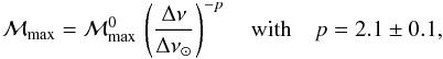 (7)where
 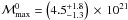 kg, and Δν is given by the scaling relation of Eq. (4).
By using Eqs. (6) and (7), the maximum of the ratio  then varies according to:
 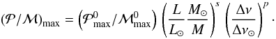 (8)
(8)
2.3. Scaling relation for Vmax
Equation (8) now permits us to proceed by considering the scaling law for mode amplitudes, in terms of surface velocities. The maximum of the mode surface velocity, by using Eq. (8) together with Eq. (1), reads 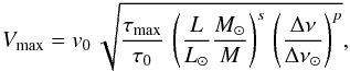 (9)where τmax is the characteristic lifetime at ν = νmax, and
  (10)with τ0 a reference mode lifetime whose values are arbitrary fixed to the lifetime of the solar radial modes at the peak frequency, that is τ0 = 3.88 days. Accordingly, we have v0 = 0.41 m/s.
It is worthwhile to note that our scaling relation (Eq. (9)) differs from the result of Kjeldsen & Bedding (2011). This is explained by the fact that the postulated relation of Kjeldsen & Bedding (2011) for mode amplitudes in velocity (their Eq. (16)) does not take the mode masses into account, while this is definitively necessary as seen in Eq. (1).
2.4. Scaling relation for bolometric amplitude
The instantaneous bolometric mode amplitude is deduced at the photosphere according to (Dziemblowski 1977; Pesnell 1990)  (11)where δL(t) is the mode Lagrangian (bolometric) luminosity perturbation, δTeff(t) the effective temperature fluctuation, and δR ∗ (t) the variation of the stellar radius.
Since the second term of Eq. (11) is found negligible in front of δTeff(t), one obtains the rms bolometric amplitudes according to  (12)where the subscript rms denotes the root mean-square.
We now need a relation between  (or equivalently
  ) and the rms mode velocity Vmax. For convenience we introduce the dimensionless coefficient ζ defined according to
  (13)where
  ppm is the maximum of the solar bolometric mode amplitude (Michel et al. 2009),
  K the effective temperature of the Sun, and
  cm/s the maximum of the solar mode (intrinsic) surface velocity evaluated at the photosphere as explained in Samadi et al. (2010).
The quantity ζ in Eq. (13) is defined at an arbitrary layer, which is generally the photosphere (i.e. at r = R ∗ ). Accordingly, we must evaluate the velocity and hence the mode mass ℳ at that layer. This implies the following scaling for ℳmax:  (14)where p ∗ = 2.0 ± 0.10,
  kg and Δν is given by the scaling relation of Eq. (4).
Combining Eq. (13) with (9) gives the scaling for the bolometric amplitude  (15)where
  m/s.
m/s.
2.4.1. Adiabatic case
Within the adiabatic approximation, it is possible to relate the mode surface velocity to intensity perturbations (e.g., Kjeldsen & Bedding 1995); this give:  (16)which assumes that the modes are quasi-adiabatic, but not only. It supposes that the modes propagate at the surface where they are measured. This approximation is not valid in the region where the modes are measured since in this region they are evanescent. Furthermore, it assumes an isothermal atmosphere. A more sophisticated quasi-adiabatic approach has been proposed by Severino et al. (2008). The authors went beyond the approximation of isothermal atmosphere by taking into account the temperature gradient as well as the fact that the intensity is measured at constant instantaneous optical depth. Both effects are taken into account by the method described in Sect. 2.4.2, which in addition considers non-adiabatic modes.
We present in Fig. 2ζK95 as a function of (L/M). The adiabatic coefficient remains almost constant for the type of stars investigated here (sub- and red giant stars). This is obviously because ζK95 varies as the inverse of the square root of Teff.
2.4.2. Non-adiabatic case
We also computed ζ using the MAD non-adiabatic pulsation code (Grigahcène et al. 2005). This code includes the time-dependent convection (TDC) treatment described in Grigahcène et al. (2005).
This TDC formulation involves a free parameter β, which takes complex values and enters the perturbed energy equation. This parameter was introduced to prevent the occurrence of non-physical spatial oscillations in the eigenfunctions (see Grigahcène et al. 2005, for details). To constrain this parameter we used the scaling relation between the frequency of the maximum height in the power spectrum (νmax) and the cut-off frequency (νc). When scaled to the Sun, one can use this scaling to infer νmax for the models we used and the parameter β is then adjusted so that the plateau (or depression) of the computed damping rates coincides (see Belkacem et al. 2012).
Note also that TDC is a non-local formulation of convection and is based on the Gabriel (1996) formalism as explained in Dupret et al. (2006b) and Dupret et al. (2006a). In this framework, non-local parameters related to the convective flux (a) and the turbulent pressure (b) are chosen in the same way as in Dupret et al. (2006b, see their Eqs. (17) and (18), see also Dupret et al. 2006c so that it fits the solar 3D numerical simulation. This calibration results in a = 10.4 and b = 2.9 (assuming a mixing-length parameter α = 1.62).
For sub- and red giant stars (L/M ≳ 10 L⊙/M⊙), the non-adiabatic intensity-velocity relation obtained with the MAD code can quite well be fitted by a power law of the form  (17)where k = 0.25 ± 0.05 and ζ0 = 0.59 ± 0.07. For main-sequence stars (L/M ≲ 10 L⊙/M⊙), ζnad remains almost constant (not shown). For the Sun, we find ζnad ≃ 0.95, which is close to the value expected by definition for the Sun. Therefore, we are then led to multiply ζnad by only a factor 1.05 so that, for the Sun, theoretical
  matches the helioseismic measurements. The result is shown in Fig. 2 for the sub- and red giant stars (L/M ≳ 10 (L⊙/M⊙)). The non-adiabatic coefficient increases rapidly with increasing (L/M) while ζK95 remains almost constant. Hence, the higher (L/M), the larger the difference between the non-adiabatic and the adiabatic coefficient (ζK95).
 |
Fig. 2 Coefficient ζ (see Eq. (13)) as a function of L/M for sub- and red giants. The filled circles correspond to the values, ζnad, obtained with the MAD non-adiabatic pulsation code (see details in the text). The empty squares correspond to the adiabatic coefficient Kjeldsen & Bedding (1995) (see Eq. (16)). The red line corresponds to a power law of the form ζ0 (L/M)k with k = 0.25. Both intensity-velocity relations ζ have been calibrated so that for the Sun ζ = 1 (see text). |
3. Comparison with the observations
We compare in this section theoretical mode amplitudes with seismic measurements made from the ground in terms of Doppler velocity (Sect. 3.2) and from space by CoRoT in terms of intensity (Sect. 3.3). We recall that computing the theoretical mode amplitudes requires knowledge of τmax (see Eqs. (9) and (15)), which is obtained from a set of CoRoT targets as explained in Sect. 3.1.
3.1. The CoRoT data set
Baudin et al. (2011) have measured the mode amplitudes for 360 CoRoT red giant targets. Among those targets, many show very narrow peaks, close to the frequency resolution of the spectrum, while the others have resolved peaks. About 65% of those targets have a highest mode whose width is sufficiently broad to be fitted with a Lorentzian profile. For those targets, the height of the highest mode, Hmax, and its lifetime τmax are thus derived from the fit procedure. However, it is not excluded that some modes with a width more narrow than the frequency resolution may have been fitted with a Lorentzian profile because of the low signal-to-noise ratio. To exclude those modes, we only considered modes with a width Γmax = 1/(πτmax) broader than twice the frequency resolution of the spectra (which is 0.081 μHz). This subset represents about 170 targets for which we have an estimate of the mode lifetime (τmax) at the peak frequency. For each target of this subset, the maximum of the mode amplitude in intensity (Amax) was obtained according to the relation  . Finally, a bolometric correction was applied in the manner of Michel et al. (2009) to convert the apparent intensity fluctuation Amax into a bolometric amplitude (δL/L)max.
3.2. Maximum velocity amplitude (Vmax)
The mode amplitude in terms of velocity is given by Eq. (9). Calculating Vmax requires to know the mode life time τmax at the peak frequency. We used the values of τmax available for our set of CoRoT targets (see Sect. 3.1). We also determined the ratio L/M as well as Δν. The luminosity and mass of these targets are unknown. However, Baudin et al. (2011) have proposed to derive an estimate of the ratio L/M using the following scaling:  (18)where νmax is the frequency of the maximum mode height Hmax and Teff is determined from photometric broad-band measurements as explained in Baudin et al. (2011). Note that the scaling law of Eq. (18) assumes that νmax scales as νc, which scales as
  (see Eq. (3)). Concerning Δν, as first established by Stello et al. (2009), Hekker et al. (2009) and Kallinger et al. (2010), there is a clear scaling relation between this quantity and νmax. We derived this quantity here according to the relation derived by Mosser et al. (2010) from a large set of CoRoT red giant stars:
  (19)Theoretical values of Vmax were compared with the stars whose Vmax has been measured so far in Doppler velocity from the ground. We considered the different measurements published in the literature (Frandsen et al. 2002; Barban et al. 2004; Bouchy et al. 2005; Carrier et al. 2005a,b; Mosser et al. 2005, 2008; Arentoft et al. 2008; Kjeldsen et al. 2008; Teixeira et al. 2009; Ando et al. 2010). The values quoted in the literature are generally given in terms of peak amplitudes. In that case they were converted into root-mean-square (rms) amplitudes. Furthermore, we rescaled all amplitudes into intrinsic (by opposition to observed) amplitudes. Measured values of Vmax are shown in Fig. 3 (top panel) as a function of L/M. We have an estimate of the ratio L/M for only a few stars while for almost all of them we have a seismic measure of νmax, which is typically more accurate than the determination of the ratio L/M. Therefore, we also show Vmax in Fig. 3 (bottom) as a function of νmax. The theoretical values of Vmax obtained for our subset of red giants are found to be close to the measurements obtained for the red giant stars observed in Doppler velocity from the ground. Note that the considerable dispersion seen in the theoretical values of Vmax comes from the dispersion in the measured value of τmax. Furthermore, we point out that the parameters p, s,
  , and ℳ0, which appear in Eq. (8), are mostly determined with quite a large error. The errors associated with the parameters introduce a bias on the theoretical Vmax, which is shown in Fig. 3 by a red vertical bar. As seen in Fig. 3, the theoretical Vmax are found, on average, to be about 30% lower than the measurements.
Using several 3D simulations of the surface of main-sequence stars, Samadi et al. (2007) have found that Vmax scales as (L/M)sv with sv = 0.7. As seen in Fig. 3, this scaling law reproduces the MS stars quite well. When extrapolated to the red giant domain (L/M ≳ 10 L⊙/M⊙), this scaling law results for Vmax in values very close to our present theoretical calculations.
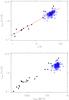 |
Fig. 3 Top: maximum of the mode velocity Vmax as a function of L/M. The filled circles correspond to the MS stars observed in Doppler velocity from the ground and the red line to the power law of the form (L/M)0.7 obtained by Samadi et al. (2007) using 3D models of MS stars. The blue squares correspond to the theoretical Vmax derived according to Eq. (9) (see Sect. 3.2). The red square corresponds to the median value of the theoretical Vmax and the associated vertical bar corresponds to bias introduced by the 1-σ error associated with the parameters p, s, |
The mode masses ℳmax were so far evaluated a the reference optical depth τ 500 nm = 0.013 (see Sect. 2.1). We now discuss the sensitivity ℳmax to the optical depth at which they are computed. To evaluate our sensitivity to this choice, we alternatively computed the theoretical Vmax at the photosphere and at an optical depth ten times lower than our reference level, that is at τ 500 nm = 10-3. Theoretical Vmax are found to be ~30% lower at the photosphere and higher by ~20% at the optical depth τ 500 nm = 10-3. This result illustrates at which level Vmax is sensitive to the depth where the acoustic modes are supposed to be measured. This depth is not well known, however, but we believe that it should be located between the photosphere and our reference optical depth.
3.3. Maximum bolometric amplitude ((δL/L)max)
3.3.1. Adiabatic case
We computed (δL/L)max according to Eq. (15) using the scaling law given by Eq. (9) for v and assuming the adiabatic coefficient ζK95 (Eq. (16)). Figure 4 (top) shows (δL/L)max as a function of ratio (L/M), where this ratio is estimated according to Eq. (18). We also plotted the mode amplitudes measured for a small sample of CoRoT main-sequence stars (see Baudin et al. 2011, and references therein). Theoretical (δL/L)max under-estimates the amplitudes measured on the CoRoT red giant stars by a factor of about 2.5.
 |
Fig. 4 Top: maximum of the mode intensity fluctuation (δL/L)max as a function of L/M. The filled circles correspond to the seismic measurements performed by Baudin et al. (2011) on a large number of CoRoT red giant stars (~170 targets). We only considered the targets for which the mode line width is broader than twice the frequency resolution (see Sect. 3.1). The empty circles correspond to the MS stars observed so far by CoRoT (see Baudin et al. 2011), and the blue squares are the theoretical (δL/L)max computed according to the Kjeldsen & Bedding (1995) adiabatic coefficient (Eq. (16), see Sect. 3.3.1). The red square corresponds to the median value of the theoretical |
3.3.2. Non-adiabatic case
We computed (δL/L)max according to Eq. (15) assuming the non-adiabatic scaling law established in Sect. 2.4.2 (see Eq. (17)) for ζ. The result is shown in Fig. 4 (bottom). Using the non-adiabatic coefficient results in an increase of the bolometric amplitude by a factor ~1.5 compared to the calculations based on the adiabatic coefficient. This renders the theoretical bolometric amplitude closer to the observations.
We have plotted in Fig. 5 the histogram of the relative difference between observed and theoretical , that is, the histogram of the quantity γ ≡ (Aobs − A)/A, where A is the theoretical amplitude and Aobs the observed one. The dispersion seen in the histogram is due both to the errors associated with the data and the fact that we observe a heterogeneous population of stars with different chemical abundance.
The red horizontal bar shows the bias introduced by the 1-σ errors associated with the determination of the parameters p ∗ , s, , ℳ0, ∗ , k, and ζ0 as well the measurement of  and
and  (see Eq. (13)). The median of γ is close to 0.8 (the vertical dashed line). This means that theoretical amplitudes remains, on average, ~40% below the CoRoT measurements.
 |
Fig. 5 Histogram of the relative difference (γ) between observed and theoretical |
4. Conclusion
4.1. Theoretical scaling relation for the velocity mode amplitude
We have extended the calculations performed by Samadi et al. (2007) for main-sequence stars to sub- and red giant stars. We found that the maximum of the mode excitation rate,  , scales approximately as (L/M)s with s = 2.60 ± 0.08. Accordingly, for sub- and red giant stars, theoretical scales in same way as for the main-sequence stars.
We also found that the mode mass at the peak frequency, ℳmax, which was evaluated at a reference level in the atmosphere, scales as Δν − p where Δν ∝ (M/R3)1/2, with p = 2.1 ± 0.1. Since (M/R3) represents also the mean density, we have that ℳmax scales almost linearly as the inverse of the star mean density. This tight relation still remains to be understood, however.
From the scaling laws for ℳmax and , we finally derived a scaling law for the maximum of the mode velocity, which has the following form: 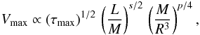 (20)where τmax is the mode lifetime at the peak frequency.
Using CoRoT data, Baudin et al. (2011) have found that τmax scales approximately as  where m = 16.2 ± 2 for the main-sequence and sub-giant stars. Recently, Appourchaux et al. (2012) have found a slope m = 15.5 ± 1.6 with Kepler data, which is hence compatible with that of Baudin et al. (2011). Such a power law is also supported by the theoretical calculations of Belkacem et al. (2012) performed for main-sequence, sub- and red giant stars. Furthermore, although ℳmax scales better with Δν, it also scales well as g − p′ with p′ = 1.66 ± 0.15 (note the larger uncertainty for p′ compared to p). Accordingly, since
  , we can rewrite the scaling for Vmax (Eq. (20)) as a function of the star spectroscopic parameters only:
  (21)Using a set of CoRoT red giant stars for which the mode lifetimes have been measured (Baudin et al. 2011), we derived from the scaling law of Eq. (20) theoretical values of Vmax. These values were found to be close to the measurements made from the ground in terms of Doppler velocity for red giant stars. However, the Doppler measurements remain on average under-estimated by a about 30%. We discuss in Sect. 5 possible reasons for this under-estimation.
4.2. Theoretical scaling relation for the bolometric mode amplitude
When converted in terms of intensity using the Kjeldsen & Bedding (1995) adiabatic relation, the theoretical amplitudes under-estimate the bolometric mode amplitudes measured by Baudin et al. (2011) on a set of CoRoT red giant stars by a factor about 2.5. Alternatively, we have considered the MAD non-adiabatic pulsation code (Grigahcène et al. 2005) to establish a non-adiabatic relation between intensity and velocity. We found that this relation scales as (L/M)k with k = 0.25 ± 0.05. We finally established for the mode amplitude in intensity the following scaling law: 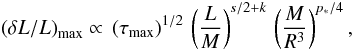 (22)where p ∗ = 2.0 ± 0.1. As for the scaling relation for Vmax, the one for
  can be rewritten as a function of the star spectroscopic parameters only:
  (23)where
  .
.
Using the non-adiabatic scaling law for reduces the difference between theoretical and measured amplitudes by a factor ~1.5. Our analysis hence explains qualitatively the recent results obtained for red giant stars using photometric CoRoT and Kepler observations (Baudin et al. 2011; Huber et al. 2011; Stello et al. 2011; Mosser et al. 2012). Indeed, we stress that theoretical relation obtained for mode amplitudes in velocity cannot be simply extrapolated into photometry because non-adiabatic effects dominate the relation between mode amplitude in velocity and intensity.
However, while the non-adiabatic treatment implemented in the MAD code (Grigahcène et al. 2005) reduces the discrepancy with the CoRoT measurements, the latter are still underestimated on average by about 40%. Possible reasons for this discrepancy are discussed in Sect. 5.
5. Discussion
The mode masses are sensitive to the layer at which they are evaluated, which must in principle correspond to the height in the atmosphere at which spectrographs dedicated to stellar seismology are the most sensitive (see Sects. 2.1, 3.2, and Samadi et al. 2008). However, the uncertainty associated with the lack of knowledge of this layer introduces an uncertainty on the computed amplitudes that should not exceed ~30% (see Sect. 3.2).
The discrepancy with the velocity measurements can also be attributed to the under-estimation of the mode driving. It is not clear which part of the excitation model might be incorrect or incomplete. Nevertheless, we believe that a possible bias can arise from the way oscillations are currently treated in the region where the driving is the most efficient (i.e. the uppermost part of the convective region). Indeed, in this region the oscillation period, the thermal time-scale and the dynamical time-scale are of the same order, making the coupling between pulsation and convection stronger and energy losses more significant (see e.g. Belkacem et al. 2011, and references therein). We have compared non-adiabatic and adiabatic eigenfunctions computed for the global standard 1D model. The non-adiabatic eigenfunctions obtained with the MAD pulsation code differ from the adiabatic ones only in a small fraction of the excitation region. We found a negligible difference between excitation rates computed with non-adiabatic eigenfunctions and those computed with adiabatic eigenfunctions. However, we point out that the underlying theory is based on a time-dependent version of the mixing-length theory, which is well known to be a crude formulation of convection. Therefore a more realistic and consistent non-adiabatic approach that does not rely on free parameters and that includes constraints from 3D hydrodynamical models is required.
Finally, part of the differences with amplitudes measured by CoRoT can be attributed to the intensity-velocity relation. Indeed, if we suppose that the mode masses are correct, then we must multiply the mode excitation rates by a factor ~1.52 = 2.25 to match the velocity measurements. In that case only a difference of about 20% with the observed remains, which must then be attributed to the intensity-relation. The intensity-relation strongly depends on the way non-adiabatic effects are treated, and as mentioned above, the current non-adiabatic treatment is based on a crude description of the convection and its inter-action with pulsation.
Acknowledgments
The CoRoT space mission, launched on December 27, 2006, has been developed and is operated by CNES, with the contribution of Austria, Belgium, Brasil, ESA, Germany and Spain.
References
- Ando, H., Tsuboi, Y., Kambe, E., & Sato, B. 2010, PASJ, 62, 1117 [NASA ADS] [Google Scholar]
- Appourchaux, T., Benomar, O., Gruberbauer, M., et al. 2012, A&A, 537, A134 [NASA ADS] [CrossRef] [EDP Sciences] [Google Scholar]
- Arentoft, T., Kjeldsen, H., Bedding, T. R., et al. 2008, ApJ, 687, 1180 [NASA ADS] [CrossRef] [Google Scholar]
- Asplund, M., Grevesse, N., & Sauval, A. J. 2005, in Cosmic Abundances as Records of Stellar Evolution and Nucleosynthesis, eds. T. G. Barnes, III, & F. N. Bash, ASP Conf. Ser., 336, 25 [Google Scholar]
- Barban, C., de Ridder, J., Mazumdar, A., et al. 2004, in Proceedings of the SOHO 14/GONG 2004 Workshop, ESA SP-559, Helio- and Asteroseismology: Towards a Golden Future 12–16 July, New Haven, Connecticut, USA, ed. D. Danesy, 113 [Google Scholar]
- Barban, C., Matthews, J. M., de Ridder, J., et al. 2007, A&A, 468, 1033 [NASA ADS] [CrossRef] [EDP Sciences] [Google Scholar]
- Baudin, F., Barban, C., Belkacem, K., et al. 2011, A&A, 529, A84 [NASA ADS] [CrossRef] [EDP Sciences] [Google Scholar]
- Bedding, T. R., Huber, D., Stello, D., et al. 2010, ApJ, 713, L176 [NASA ADS] [CrossRef] [Google Scholar]
- Belkacem, K., Samadi, R., Goupil, M. J., et al. 2010, A&A, 522, L2 [NASA ADS] [CrossRef] [EDP Sciences] [Google Scholar]
- Belkacem, K., Goupil, M. J., Dupret, M. A., et al. 2011, A&A, 530, A142 [Google Scholar]
- Belkacem, K., Dupret, M. A., Baudin, F., et al. 2012, A&A, 540, L7 [NASA ADS] [CrossRef] [EDP Sciences] [Google Scholar]
- Bouchy, F., Bazot, M., Santos, N. C., Vauclair, S., & Sosnowska, D. 2005, A&A, 440, 609 [NASA ADS] [CrossRef] [EDP Sciences] [Google Scholar]
- Canuto, V. M., Goldman, I., & Mazzitelli, I. 1996, ApJ, 473, 550 [NASA ADS] [CrossRef] [Google Scholar]
- Carrier, F., Eggenberger, P., & Bouchy, F. 2005a, A&A, 434, 1085 [NASA ADS] [CrossRef] [EDP Sciences] [Google Scholar]
- Carrier, F., Eggenberger, P., D’Alessandro, A., & Weber, L. 2005b, New A, 10, 315 [Google Scholar]
- Chaplin, W. J., Houdek, G., Elsworth, Y., et al. 2005, MNRAS, 360, 859 [NASA ADS] [CrossRef] [Google Scholar]
- Christensen-Dalsgaard, J. 1982, MNRAS, 199, 735 [Google Scholar]
- Christensen-Dalsgaard, J. 2008, Ap&SS, 316, 113 [NASA ADS] [CrossRef] [Google Scholar]
- de Ridder, J., Barban, C., Baudin, F., et al. 2009, Nature, 459, 398 [Google Scholar]
- Dupret, M. A., Barban, C., Goupil, M.-J., et al. 2006a, in Proceedings of SOHO 18/GONG 2006/HELAS I, Beyond the spherical Sun, ESA Spec. Publ., 624 [Google Scholar]
- Dupret, M.-A., Goupil, M.-J., Samadi, R., Grigahcène, A., & Gabriel, M. 2006b, in Proceedings of SOHO 18/GONG 2006/HELAS I, Beyond the spherical Sun, ESA Spec. Publ., 624 [Google Scholar]
- Dupret, M.-A., Samadi, R., Grigahcene, A., Goupil, M.-J., & Gabriel, M. 2006c, Commun. Asteroseismol., 147, 85 [NASA ADS] [CrossRef] [Google Scholar]
- Dziemblowski, W. 1977, Acta Astron., 27, 95 [NASA ADS] [Google Scholar]
- Frandsen, S., Carrier, F., Aerts, C., et al. 2002, A&A, 394, L5 [NASA ADS] [CrossRef] [EDP Sciences] [Google Scholar]
- Freytag, B., Steffen, M., & Dorch, B. 2002, Astron. Nachr., 323, 213 [NASA ADS] [CrossRef] [EDP Sciences] [Google Scholar]
- Freytag, B., Steffen, M., Ludwig, H.-G., et al. 2012, J. Comput. Phys., 231, 919 [Google Scholar]
- Gabriel, M. 1996, BASI, 24, 233 [Google Scholar]
- Goldreich, P., & Keeley, D. A. 1977, ApJ, 212, 243 [NASA ADS] [CrossRef] [Google Scholar]
- Goldreich, P., Murray, N., & Kumar, P. 1994, ApJ, 424, 466 [NASA ADS] [CrossRef] [Google Scholar]
- Grigahcène, A., Dupret, M.-A., Gabriel, M., Garrido, R., & Scuflaire, R. 2005, A&A, 434, 1055 [NASA ADS] [CrossRef] [EDP Sciences] [Google Scholar]
- Hekker, S., Kallinger, T., Baudin, F., et al. 2009, A&A, 506, 465 [NASA ADS] [CrossRef] [EDP Sciences] [Google Scholar]
- Huber, D., Bedding, T. R., Stello, D., et al. 2010, ApJ, 723, 1607 [NASA ADS] [CrossRef] [Google Scholar]
- Huber, D., Bedding, T. R., Stello, D., et al. 2011, ApJ, 743, 143 [NASA ADS] [CrossRef] [Google Scholar]
- Jiménez, A. 2006, ApJ, 646, 1398 [NASA ADS] [CrossRef] [Google Scholar]
- Kallinger, T., Weiss, W. W., Barban, C., et al. 2010, A&A, 509, A77 [NASA ADS] [CrossRef] [EDP Sciences] [Google Scholar]
- Kjeldsen, H., & Bedding, T. R. 1995, A&A, 293, 87 [NASA ADS] [Google Scholar]
- Kjeldsen, H., & Bedding, T. R. 2011, A&A, 529, L8 [NASA ADS] [CrossRef] [EDP Sciences] [Google Scholar]
- Kjeldsen, H., Bedding, T. R., Arentoft, T., et al. 2008, ApJ, 682, 1370 [NASA ADS] [CrossRef] [Google Scholar]
- Michel, E., Samadi, R., Baudin, F., et al. 2009, A&A, 495, 979 [NASA ADS] [CrossRef] [EDP Sciences] [Google Scholar]
- Miglio, A., Montalbán, J., Baudin, F., et al. 2009, A&A, 503, L21 [NASA ADS] [CrossRef] [EDP Sciences] [MathSciNet] [Google Scholar]
- Morel, P., & Lebreton, Y. 2008, Ap&SS, 316, 61 [NASA ADS] [CrossRef] [MathSciNet] [Google Scholar]
- Mosser, B., Bouchy, F., Catala, C., et al. 2005, A&A, 431, L13 [NASA ADS] [CrossRef] [EDP Sciences] [Google Scholar]
- Mosser, B., Deheuvels, S., Michel, E., et al. 2008, A&A, 488, 635 [NASA ADS] [CrossRef] [EDP Sciences] [Google Scholar]
- Mosser, B., Belkacem, K., Goupil, M.-J., et al. 2010, A&A, 517, A22 [NASA ADS] [CrossRef] [EDP Sciences] [Google Scholar]
- Mosser, B., Elsworth, Y., Hekker, S., et al. 2012, A&A, 537, A30 [NASA ADS] [CrossRef] [EDP Sciences] [Google Scholar]
- Pesnell, W. D. 1990, ApJ, 363, 227 [NASA ADS] [CrossRef] [Google Scholar]
- Samadi, R. 2011, in Lect. Notes Phys., 832, 305 [Google Scholar]
- Samadi, R., & Goupil, M. J. 2001, A&A, 370, 136 [NASA ADS] [CrossRef] [EDP Sciences] [Google Scholar]
- Samadi, R., Georgobiani, D., Trampedach, R., et al. 2007, A&A, 463, 297 [NASA ADS] [CrossRef] [EDP Sciences] [Google Scholar]
- Samadi, R., Belkacem, K., Goupil, M. J., Dupret, M.-A., & Kupka, F. 2008, A&A, 489, 291 [NASA ADS] [CrossRef] [EDP Sciences] [Google Scholar]
- Samadi, R., Ludwig, H.-G., Belkacem, K., et al. 2010, A&A, 509, A16 [NASA ADS] [CrossRef] [EDP Sciences] [Google Scholar]
- Severino, G., Straus, T., & Steffen, M. 2008, Sol. Phys., 251, 549 [Google Scholar]
- Stein, R., Georgobiani, D., Trampedach, R., Ludwig, H.-G., & Nordlund, Å. 2004, Sol. Phys., 220, 229 [NASA ADS] [CrossRef] [Google Scholar]
- Stello, D., Chaplin, W. J., Basu, S., Elsworth, Y., & Bedding, T. R. 2009, MNRAS, 400, L80 [NASA ADS] [CrossRef] [Google Scholar]
- Stello, D., Huber, D., Kallinger, T., et al. 2011, ApJ, 737, L10 [NASA ADS] [CrossRef] [Google Scholar]
- Teixeira, T. C., Kjeldsen, H., Bedding, T. R., et al. 2009, A&A, 494, 237 [NASA ADS] [CrossRef] [EDP Sciences] [Google Scholar]
- Toutain, T., & Froehlich, C. 1992, A&A, 257, 287 [NASA ADS] [Google Scholar]
- Wedemeyer, S., Freytag, B., Steffen, M., Ludwig, H.-G., & Holweger, H. 2004, A&A, 414, 1121 [NASA ADS] [CrossRef] [EDP Sciences] [Google Scholar]
All Tables
All Figures
|
Fig. 1 Top: |
| In the text | |
|
Fig. 2 Coefficient ζ (see Eq. (13)) as a function of L/M for sub- and red giants. The filled circles correspond to the values, ζnad, obtained with the MAD non-adiabatic pulsation code (see details in the text). The empty squares correspond to the adiabatic coefficient Kjeldsen & Bedding (1995) (see Eq. (16)). The red line corresponds to a power law of the form ζ0 (L/M)k with k = 0.25. Both intensity-velocity relations ζ have been calibrated so that for the Sun ζ = 1 (see text). |
| In the text | |
|
Fig. 3 Top: maximum of the mode velocity Vmax as a function of L/M. The filled circles correspond to the MS stars observed in Doppler velocity from the ground and the red line to the power law of the form (L/M)0.7 obtained by Samadi et al. (2007) using 3D models of MS stars. The blue squares correspond to the theoretical Vmax derived according to Eq. (9) (see Sect. 3.2). The red square corresponds to the median value of the theoretical Vmax and the associated vertical bar corresponds to bias introduced by the 1-σ error associated with the parameters p, s, |
| In the text | |
|
Fig. 4 Top: maximum of the mode intensity fluctuation (δL/L)max as a function of L/M. The filled circles correspond to the seismic measurements performed by Baudin et al. (2011) on a large number of CoRoT red giant stars (~170 targets). We only considered the targets for which the mode line width is broader than twice the frequency resolution (see Sect. 3.1). The empty circles correspond to the MS stars observed so far by CoRoT (see Baudin et al. 2011), and the blue squares are the theoretical (δL/L)max computed according to the Kjeldsen & Bedding (1995) adiabatic coefficient (Eq. (16), see Sect. 3.3.1). The red square corresponds to the median value of the theoretical |
| In the text | |
|
Fig. 5 Histogram of the relative difference (γ) between observed and theoretical |
| In the text | |
Current usage metrics show cumulative count of Article Views (full-text article views including HTML views, PDF and ePub downloads, according to the available data) and Abstracts Views on Vision4Press platform.
Data correspond to usage on the plateform after 2015. The current usage metrics is available 48-96 hours after online publication and is updated daily on week days.
Initial download of the metrics may take a while.