| Issue |
A&A
Volume 543, July 2012
|
|
|---|---|---|
| Article Number | A48 | |
| Number of page(s) | 26 | |
| Section | Interstellar and circumstellar matter | |
| DOI | https://doi.org/10.1051/0004-6361/201218963 | |
| Published online | 26 June 2012 | |
Molecular abundances in the inner layers of IRC +10216⋆,⋆⋆
1 Departamento de Astrofísica, Centro de Astrobiología, CSIC–INTA, Ctra. de Torrejón a Ajalvir km 4, 28850 Madrid Spain
2 Univ. Bordeaux, LAB, UMR 5804, 33270 Floirac, France
e-mail: Marcelino.Agundez@obs.u-bordeaux1.fr
3 CNRS, LAB, UMR 5804, 33270 Floirac, France
4 Departamento de Estrellas y Medio Interestelar, Instituto de Astronomía, Universidad Nacional Autónoma de México, Ciudad Universitaria, 04510 México City, Mexico
5 Institut de Planétologie et d’Astrophysique de Grenoble (IPAG), Univ. J. Fourier and CNRS (UMR 5274), BP 53, 38041 Grenoble Cedex 9, France
6 Institut de Radioastronomie Millimétrique, 300 rue de la Piscine, 38406 Saint-Martin d’Hères, France
Received: 4 February 2012
Accepted: 16 April 2012
Context. The inner layers of circumstellar envelopes around asymptotic giant branch stars are sites where a variety of processes such as thermochemical equilibrium, shocks induced by the stellar pulsation, and condensation of dust grains determine the chemical composition of the material that is expelled into the outer envelope layers and, ultimately, into interstellar space.
Aims. We aim at studying the abundances, throughout the whole circumstellar envelope of the carbon star IRC +10216, of several molecules formed in the inner layers in order to constrain the different processes at work in such regions.
Methods. Observations towards IRC +10216 of CS, SiO, SiS, NaCl, KCl, AlCl, AlF, and NaCN have been carried out with the IRAM 30-m telescope in the 80−357.5 GHz frequency range. A large number of rotational transitions covering a wide range of energy levels, including highly excited vibrational states, are detected in emission and serve to trace different regions of the envelope. Radiative transfer calculations based on the LVG formalism have been performed to derive molecular abundances from the innermost out to the outer layers. The excitation calculations include infrared pumping to excited vibrational states and inelastic collisions, for which up-to-date rate coefficients for rotational and, in some cases, ro-vibrational transitions are used.
Results. We find that in the inner layers CS, SiO, and SiS have abundances relative to H2 of 4 × 10⁻⁶, 1.8 × 10⁻⁷, and 3 × 10⁻⁶, respectively, and that CS and SiS have significant lower abundances in the outer envelope, which implies that they actively contribute to the formation of dust. Moreover, in the inner layers, the amount of sulfur and silicon in gas phase molecules is only 27% for S and 5.6% for Si, implying that these elements have already condensed onto grains, most likely in the form of MgS and SiC. Metal-bearing molecules lock up a relatively small fraction of metals, although our results indicate that NaCl, KCl, AlCl, AlF, and NaCN, despite their refractory character, are not significantly depleted in the cold outer layers. In these regions a few percent of the metals Na, K, and Al survive in the gas phase, either in atomic or molecular form, and are therefore available to participate in the gas phase chemistry in the outer envelope.
Key words: astrochemistry / line: identification / molecular processes / stars: AGB and post-AGB / circumstellar matter / stars: individual: IRC +10216
Based on observations carried out with the IRAM 30-m telescope. IRAM is supported by INSU/CNRS (France), MPG (Germany), and IGN (Spain).
Tables 1–8 are available in electronic form at http://www.aanda.org
© ESO, 2012
1. Introduction
The carbon star envelope IRC +10216 is among the best studied astronomical objects (Morris 1975; Glassgold 1996; Mauron & Huggins 1999; Cernicharo et al. 2000; Millar et al. 2000). The central low-mass asymptotic giant branch (AGB) star CW Leo, losing mass at a high rate (1 − 4 × 10⁻⁵ M⊙ yr-1), is embedded in a dense and nearly spherical circumstellar envelope composed of molecular gas and dust particles. Being a relatively nearby source (110 − 170 pc), it is one of the brightest infrared objects and richest molecular sources – with more than 80 molecules detected – in the sky. IRC +10216 is the prototype of carbon star and a challenging source for chemical models.
Molecules observed in IRC +10216 form either in the atmosphere of the central AGB star, from where they are expelled (parent species) or in situ in the outer envelope (daughter species). Interferometric maps show that molecular emission peaks either on the star or farther out in a hollow shell of radius 10 − 20′′ (Lucas et al. 1995; Guélin et al. 1997). The parent species are formed in the dense and hot atmosphere at thermochemical equilibrium (TE), although the formation of dust grains, shocks, and the penetration of interstellar ultraviolet photons through the clumpy envelope (Agúndez & Cernicharo 2006; Cherchneff 2006; Agúndez et al. 2010) can make molecular abundances to deviate from TE. The chemical composition in the inner layers is key as this material, once incorporated in the outflowing wind, constitutes the basis for the rich photochemistry and ion-neutral chemistry that takes place in the outer envelope layers.
Probing molecular abundances in the warm (1000 − 2000 K) and dense (108 − 1014 cm-3) inner layers requires the observation of high energy rotational or ro-vibrational lines that lie in the submillimeter and infrared regions of the spectrum, which can hardly be observed from the ground. Efforts to this end were undertaken by Keady & Ridgway (1993) and Boyle et al. (1994), who observed with ground-based telescopes absorption lines due to ro-vibrational transitions of C2H2, CH4, SiH4, CS, SiO, NH3, and SiS near 10 and 13.5 μm. Fonfría et al. (2008) made a sensitive spectral survey in the 11 − 14 μm range that unveiled a forest of ro-vibrational lines arising from C2H2 and HCN. A recent interferometric spectral survey in the 0.9 mm atmospheric window by Patel et al. (2011) allowed to detect a good number of narrow unidentified lines arising from the innermost envelope, inside the acceleration region, that they tentatively assign to molecular rotational transitions within excited vibrational states.
Space missions now freely explore spectral regions not accessible from the ground. ISO observed a full infrared scan from 2.4 to 197 μm, albeit with a low spatial and spectral resolution, that probed the inner layers of IRC +10216 through the lines of abundant molecules such as CO, C2H2, and HCN (Cernicharo et al. 1996, 1999). More recently, spectral surveys carried out with Herschel with a high angular resolution have detected many high energy rotational transitions of molecules such as CO, HCN, CS, SiS, SiO, and SiC2, at low spectral resolution using SPIRE and PACS in the 55 − 672 μm range (Decin et al. 2010a), and at high spectral resolution in the 488 − 1901 GHz range covered by HIFI (Cernicharo et al. 2010).
Here we present an exhaustive analysis of the abundance and excitation conditions of several molecules formed in the inner layers of IRC +10216, based on high sensitive observations within the full frequency coverage of the IRAM 30-m telescope (80 − 360 GHz). We focus on the parent molecules CS, SiO, SiS, NaCl, KCl, AlCl, AlF, and NaCN. The cases of CO, HCN, and SiC2, also formed in the inner layers and reachable by the IRAM 30-m telescope, have been treated recently (De Beck et al. 2012; Fonfría et al. 2008; Cernicharo et al. 2010, 2011). The observation of a large number of rotational transitions covering a wide range of excitation energies coupled to radiative transfer calculations allows us to derive accurate abundances throughout the envelope. Rotational transitions of CS, SiO, and SiS in highly excited vibrational states are observed; for SiS up to v = 5, with energy levels above 3600 cm-1 (5200 K). They put severe constraints on the abundance of these species in the innermost regions. Together with low energy transitions, the abundance can be tracked from the inner to the outer layers, allowing to evaluate the effects of shocks, grain formation, and gas phase chemistry.
2. Astronomical observations
The mm-wave observations of IRC +10216 on which the present study is based were made with the IRAM 30-m telescope on Pico Veleta (Spain). They cover the main atmospheric windows, at λ3 mm (80 − 116 GHz), λ2 mm (129 − 183.5), and λ1 mm (197 − 357.5). The observations at 3 and 2 mm were carried out between 1986 and 2008 using the old ABCD SIS receivers. A large part of the λ2 mm data have been already presented as a spectral survey (Cernicharo et al. 2000). At λ3 mm, the most sensitive observations were obtained after 2002 in the context of a coherent line survey not yet published (Cernicharo et al., in prep.). Part of the spectra at 1 mm were obtained from 1999 to 2008 using the ABCD receivers although most of the data, in particular all spectra with frequencies above 258 GHz, were observed from December 2009 to December 2010 with the new low-noise wide-band EMIR receivers, in the context of a line survey (Kahane et al., in prep.).
Both the old ABCD and the new EMIR receivers are dual polarization and operate in single side band. Image side band rejections are > 20 dB at 3 mm and 2 mm, ~10 dB at 1 mm with ABCD receivers, and ≥ 10 dB at 1 mm with EMIR receivers. Identification of image side band lines during the observations with ABCD receivers was done through shifts in the local oscillator frequency. This was not necessary with EMIR receivers because of the markedly different rejection of the horizontal and vertical polarizations. The backends provided spectral resolutions between 1 and 2 MHz. The coarser resolution was used above 258 GHz where it corresponds to ≤ 2.3 km s-1, still good enough to resolve the lines in IRC +10216’s spectra which have typical widths of 20 − 30 km s-1.
The observations were made in the wobbler switching observing mode by nutating the secondary mirror by ± 90′′ or ± 120′′ at a rate of 0.5 Hz. The intensity in figures and tables is expressed in terms of  , the antenna temperature corrected for atmospheric absorption and for antenna ohmic and spillover losses. can be converted into TMB (main beam brightness temperature) by dividing by Beff/Feff, where Feff, the telescope forward efficiency, is 0.95 at 3 mm, 0.93 at 2 mm, 0.91 at 1.3 mm, and 0.88 at 1 mm for ABCD receivers, and 0.91 at 1.3 mm and 0.84 at 0.9 mm for EMIR receivers, and Beff, the beam efficiency, is given by Beff = 0.828 × exp {−(ν/341)2 } for receivers ABCD and by Beff = 0.865 × exp {−(ν/365)2 } for EMIR receivers, where ν is the frequency expressed in GHz.
The pointing and focus of the telescope were checked every 1 − 2 h on nearby planets or the quasar OJ 287. The error in the telescope pointing is estimated to be 1 − 2′′. The main beam of the IRAM 30-m telescope is given by HPBW(′′) = 2460/ν(GHz), so that it ranges from 30′′ at 80 GHz to 7′′ at 360 GHz.
IRC +10216 is a variable source with a period of 649 days and a variation in the infrared (IR) flux from maximum to minimum phase of 2.2 mag at 1.2 μm and 0.6 mag at 18 μm (Le Bertre 1992). Since our observations were carried out over a time span of several years, we checked for possible time variation in the intensity of some lines, especially those that are radiatively excited. Most of the studied lines in the λ3 and λ2 mm bands were observed at various epochs corresponding to different IR phases. As previously discussed in Cernicharo et al. (2000), we have found no evidence of time variability of the line intensities that exceeds the calibration uncertainties and could be ascribed to changes of the IR flux. Calibration uncertainties, mostly linked to corrections of atmospheric absorption and pointing errors, are estimated to be ≤10% at 3 mm, ≤20% at 2 mm, and ≤30% at 1.3 mm. Most of the lines at wavelengths shorter than 1.1 mm were observed just once, so that no constraints can be put on their time variability.
Observations of CS cover the J = 2−1 to J = 7−6 rotational transitions of the v = 0 state, some rotational transitions of the excited vibrational states v = 1,2,3, as well as several transitions of the rare isotopomers 13CS, C34S, and C33S (see Table 1). For SiO, we observed the J = 2−1 through J = 8−7 rotational transitions of the v = 0 state and 3 transitions of the v = 1 state, as well as several rotational transitions of the rare isotopomers 29SiO, 30SiO, Si18O, and Si17O (see Table 2). In the case of SiS, rotational transitions from J = 5−4 to J = 19−18 are observed in vibrational states up to v = 5. A good number of lines of the ground and excited vibrational states were also observed for the rare isotopomers 29SiS, 30SiS, Si34S, and Si33S (see Table 3). Finally, rotational transitions of several metal-bearing molecules were observed in their ground vibrational states, including the halides NaCl, KCl, AlCl, and AlF, and the cyanide NaCN. For this latter, rotational transitions with upper quantum numbers J = 5 to J = 23 and Ka = 0 to Ka = 10 were clearly detected. In the cases of the chlorine-containing molecules both the 35Cl and 37Cl isotopomers were detected (see Tables 4 − 8).
3. Physical model of IRC +10216
IRC +10216’s model parameters.
The physical model consists of a spherical envelope of gas and dust expanding around a central AGB star. The parameters adopted are given in Table 9. The assumed distance to IRC +10216 is 130 pc (Men’shchikov et al. 2001). We consider an AGB star with an effective temperature T∗ of 2330 K (Ridgway & Keady 1988), a radius R∗ of 4 × 1013 cm (0.021′′, which is consistent with the value of 0.022′′ derived from infrared interferometry by Monnier et al. 2000). The adopted values for T∗ and R∗ imply a stellar luminosity of 8750 L⊙, within the range 5200 − 13 000 L⊙ given by Men’shchikov et al. (2001). The adopted stellar mass is 0.8 M⊙ (Winters et al. 1994; Men’shchikov et al. 2001).
The dust condensation radius Rc is located at 5 R∗ and the end of the dust acceleration region Rw at 20 R∗, with the gas expansion velocity being 5 km s-1 for the regions inner to Rc, 11 km s-1 in the dust acceleration region, and 14.5 km s-1 beyond Rw (see Fig. 1), in agreement with IR studies of the inner layers of IRC +10216 (Keady & Ridgway 1993; Fonfría et al. 2008). The adopted microturbulence velocity Δvturb is 5 km s-1 at the stellar photosphere, decreasing down to 1 km s-1 at Rc (Keady et al. 1988; see Table 9). Beyond Rc we consider a constant microturbulence velocity of 1 km s-1, within the range of values 0.65 − 1.5 km s-1 derived in the literature (Skinner et al. 1999; De Beck et al. 2012).
The mass loss rate and gas kinetic temperature in the envelope are derived from the modeling of the rotational lines J = 1 − 0 to J = 16 − 15 of 12CO and 13CO observed with the IRAM 30-m telescope and HIFI (see De Beck et al. 2012). We used a non-local radiative transfer code (Daniel & Cernicharo 2008), and adopted an abundance of CO relative to H2 of 6 × 10⁻⁴ (Crosas & Menten 1997; Skinner et al. 1999) and an abundance ratio 12CO/13CO of 45 (Cernicharo et al. 2000). We derive a mass loss rate of 2 × 10⁻⁵ M⊙ yr-1, and a gas kinetic temperature that varies with radius as r-0.55 for regions inner to 75 R∗, as r-0.85 between 75 and 200 R∗, and as r-1.40 beyond 200 R∗ (see Fig. 1).
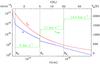 |
Fig. 1 Particle density n, gas kinetic temperature Tk, and expansion velocity vexp as a function of radius in the inner layers of IRC +10216. |
As concerns dust, we consider spherical grains of amorphous carbon with a radius of 0.1 μm, a mass density of 2 g cm-3, and the optical properties of Suh (2000). The dust continuum is modeled using a ray-tracing code that propagates the specific intensities along a set of impact parameters which are subsequently convolved with the telescope beam. The model does not include scattering, which becomes important only at short wavelengths, below 5 μm. From the modeling of the envelope spectral energy distribution (see Fig. 2) we find a gas-to-dust mass ratio of 300 and a dust temperature (Td) radial distribution of the form Td = 800 K × (r/Rc)-0.375.
 |
Fig. 2 Spectral energy distribution of IRC +10216 as observed by ISO (black line; Cernicharo et al. 1999), as given by photometric measurements (blue crossed boxes; values taken from Le Bertre 1992, and from the IRAS Point Source Catalog), and as calculated by the dust model (red line). |
The variation of the density of gas particles with radius is different depending on the region of the envelope. In the static stellar atmosphere, that extends from the photosphere up to a radius R0 which we take as 1.2 R∗, the density is given by hydrostatic equilibrium  (1)where G and k are the gravitational and Boltzmann constants, respectively, α is the exponent in the kinetic temperature law (α = 0.55), and ⟨ mg ⟩ is the mean mass of gas particles (2.3 amu, after considering H2, He, and CO). In the dynamic atmosphere shock waves induced by the pulsation of the star extend the circumstellar material. For this region, that extends from R0 up to Rc, we utilize the equation proposed by Cherchneff (1992):
 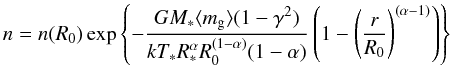 (2)where γ is a dimensionless parameter expressing the ratio of the shock strength to the local escape velocity (γ = 0.89, see Cherchneff 1992). Finally, beyond the dust condensation radius Rc, the density at each radius in the envelope is given by the law of conservation of mass
 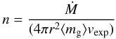 (3)which results in a density profile varying as r-2, with jumps at Rc and Rw, which reflect the jumps in the adopted expansion velocity profile (see Fig. 1).
The treatment of the density profiles is similar to that adopted in Agúndez & Cernicharo (2006), except that we have updated some parameters, such as the stellar mass, and we now do not use anymore the phenomenological parameter Kn in Eq. (2). The density scale is fixed by the mass loss rate through Eq. (3), and afterwards Eqs. (1) and (2) determine the density gradient from Rc down to the photosphere. These two latter equations involve several uncertain parameters. For example, the stellar mass is not accurately known although it can be confined to the range 0.6 − 1 M⊙, based on theoretical arguments and on the late AGB stage of IRC +10216 (Winters et al. 1994). This relatively small error on the stellar mass translates into an uncertainty of a factor of 5 for the density at R0. At this point it is worth to note that densities in the inner layers of IRC +10216 are not particularly well constrained by observations and differ by orders of magnitude between different modeling studies. For example, Willacy & Cherchneff (1998) adopted, in their chemical model of the inner wind, a density of 3 × 1011 cm-3 at 5 R∗ rising up to 4 × 1014 cm-3 at 1.2 R∗, while Schöier et al. (2006a), in their model aimed at interpreting SiO observations, adopted a value of about 2 × 108 cm-3 at 5 R∗ rising up to 3 × 1010 cm-3 close to the photosphere. In our model, densities in the inner layers are in between the two above cases, with a value of 1.8 × 1014 cm-3 at R∗, 8 × 1011 cm-3 at R0, and (0.6 − 1.3) × 109 cm-3 at Rc. The density of particles is therefore more uncertain in the inner layers than in the outer envelope, and this uncertainty translates to the molecular abundances derived (see more details in Sect. 4.3).
4. Radiative transfer modeling
The calculation of the excitation and emergent line profiles for the different molecules studied here has been done with a multi-shell radiative transfer program based on the LVG (Large Velocity Gradient) formalism, which is described in Agúndez (2009). Briefly, the spherical circumstellar envelope is divided into several concentric shells, and statistical equilibrium equations are solved in each of them. The radiation field  at the frequency ν of each transition, needed to solve the statistical equilibrium equations, is evaluated in each shell through an escape probability formalism as
  (4)where Sν is the local source function,
  is the specific intensity of the background radiation field, and β is the so-called escape probability, evaluated as (1 − e − τν)/τν for an expanding spherical shell (Castor 1970), with τν being the optical depth in the radial direction within the corresponding shell. The contributions of both gas and dust are included in the computation of Sν and τν. The background radiation field arriving at a given shell is composed of the cosmic microwave background, the stellar component (geometrically diluted and properly propagated through the inner dusty shells), and the dust emission arising from the outer shells.
Apart from the radiation at millimeter wavelengths involved in the observed rotational transitions, infrared radiation plays an important role for the excitation of some molecules through the pumping to excited vibrational states. According to the above description, the source of this infrared radiation in each shell is on one side local (emission from the warm dust contained in the shell that contributes to the local source function) and on the other side external (arising from the surrounding shells containing warm dust heated by the stellar radiation).
4.1. Molecular data
The radiative transfer calculations require as input spectroscopic and collision excitation data. Spectroscopic data has been obtained from a catalog developed by one of us (Cernicharo), which has been previously used in Cernicharo et al. (2000) and will be published soon. As concerns collision data, ideally one would need rate coefficients for inelastic collisions with H2 and He involving a large enough number of energy levels and covering a wide enough range of temperatures. Since this is not often the case, some approximations must be considered. In this study we have adopted the following rules for all the studied molecules. Inelastic collisions with both H2 and He (with an abundance of 0.17 relative to H2; Asplund et al. 2009) have been considered. When no rate coefficients for collisions with H2 were available, as is the case of CS, we scaled those calculated for He by multiplying them by the squared ratio of the reduced masses of the H2 and He colliding systems. When rate coefficients were available for both ortho and para H2, an ortho/para ratio of 3 was assumed. Wherever we needed rate coefficients involving rotational levels higher than those included in the quantum calculations, we computed them by using the infinite order sudden (IOS) approximation (Goldflam et al. 1977). No extrapolation in temperature has however been made outside the temperature validity range of the quantum calculations. Finally, the collision excitation rates have been systematically computed from the de-excitation rates applying detailed balance. More details are given below for individual molecules.
-
CS: we have considered the first 50 rotationallevels within the vibrational states v = 0−3. The level energies and transition frequencies were calculated from the Dunham coefficients provided by Müller et al. (2005), the line strengths for rotational transitions were computed from the dipole moments for each vibrational state μv = 0 = 1.985 D, μv = 1 = 1.936 D (Winnewisser & Cook 1968), μv = 2 = 1.914 D (CDMS1), and μv = 3 = 1.855 D (López Piñeiro & Tipping 1987), while for ro-vibrational transitions the Einstein coefficients were obtained from the values calculated by Chandra et al. (1995) for the P(1) transition of each vibrational band (see e.g. Tipping & Chackerian 1981). Rate coefficients for de-excitation through inelastic collisions with H2 and He were taken from Lique et al. (2006), who calculated coefficients for collisions with He including the first 31 rotational levels and up to temperatures of 300 K, and from Lique & Spielfiedel (2007), who included the first 38 rotational levels within the first 3 vibrational states and computed collision coefficients for rotational and ro-vibrational transitions at temperatures between 300 and 1500 K.
-
SiO: the first 50 rotational levels of the v = 0 and v = 1 vibrational states have been included. The Dunham coefficients given by Sanz et al. (2003), the dipole moments μv = 0 = 3.0982 D and μv = 1 = 3.1178 D measured by Raymonda et al. (1970), and the Einstein coefficient for the v = 1−0 P(1) transition calculated by Drira et al. (1997) were used to compute the line frequencies and strengths. The collision rate coefficients calculated by Dayou & Balança (2006) for the first 20 rotational levels and for temperatures up to 300 K were adopted. For temperatures higher than 300 K and for ro-vibrational transitions we adopted the collision rate coefficients used for CS.
-
SiS: we have included the first 70 rotational levels within the v = 0 − 5 vibrational states. The Dunham coefficients and the dipole moment of 1.735 D given by Müller et al. (2007), together with the dipole moments for ro-vibrational transitions given by López Piñeiro et al. (1987) have been used to compute level energies and Einstein coefficients. The rate coefficients of rotational de-excitation through collisions with He and ortho/para H2 have been taken from the calculations of Vincent et al. (2007) and Kłos & Lique (2008), which extend up to temperatures of 200 − 300 K. For higher temperatures and for ro-vibrational transitions the collision rate coefficients calculated by Toboła et al. (2008) were used.
-
Metal halides: the spectroscopic properties of NaCl, KCl, AlCl, and AlF are relatively well known (Caris et al. 2002, 2004; Hedderich et al. 1993; Hedderich & Bernath 1992). The permanent electric dipole moment is very large for NaCl (9.00117 D; De Leeuw et al. 1970) and KCl (10.269 D; van Wachen & Dymanus 1967), and noticeably smaller for AlCl and AlF, 1 − 2 D and 1.53 D, respectively (Lide 1965). For AlCl we adopted a value of 1.5 D, in agreement with the estimation of Lide (1965) and the value previously used by Cernicharo & Guélin (1987). We have not included vibrationally excited states since no lines involving such states are observed in IRC +10216, and since vibrational line strengths for those molecules are poorly known. Recently, Gotoum et al. (2011, 2012) have calculated the rate coefficients for AlF de-excitation through collisions with He and para H2 up to temperatures of 300 and 70 K, respectively. We have also used those rate coefficients for AlCl, which has a similar dipole moment than AlF. For NaCl and KCl, we have adopted the values used for SiS, which extend up to higher temperatures. The lack of accurate collision rate coefficients at high temperatures for these metal halides introduce significant uncertainties in the derived abundances.
-
NaCN: we consider rotational levels within the ground vibrational state up to J = 29. The rotational constants used to compute the level energies were derived from a fit to the line frequencies measured in the spectrum of IRC +10216 and in the laboratory by Halfen & Ziurys (2011)2. The dipole moment of NaCN is calculated to be 8.85 D (CDMS1). Due to the lack of calculated collision data for NaCN we use the following approximate formula to compute the de-excitation rate coefficients γ due to collisions with H2:
 (5)where ′ and ′′ stand for upper and lower level, respectively, and γ has units of cm3 s-1. Equation (5) gives a first approximation of collision rate coefficients for asymmetric rotors, resulting in values within one order of magnitude of those calculated for asymmetric rotors such as SO2 (Green 1995) and HCO
 (Hammami et al. 2007). We, nevertheless, note that the use of this approximate formula may introduce significant errors in the excitation and abundance of NaCN.
The lack of collision rate coefficients for AlCl, NaCl, KCl, and NaCN may introduce important uncertainties in the derived abundances. We may in fact question whether the choice of the collision rate coefficients for these molecules is more adequate than the simple assumption of local thermodynamic equilibrium (LTE). In the case of AlCl, the choice of the collision coefficients calculated for AlF does not seem a bad approach based on the similar dipole moment and mass of both molecules. In any case, the observed lines of AlCl (see discussion in Sect. 4.3) arise from regions where the level populations are very close to thermalization, and therefore both the use of collision coefficients and the LTE approach yield similar results. This is not the case for NaCl, KCl, and NaCN (see also discussion in Sect. 4.3), for which the assumption of LTE results in a very bad agreement with the observed lines (the calculated low-J lines are much too weak and the high-J lines are too strong). We are therefore confident that our choice of the collision rate coefficients for NaCl, KCl, and NaCN yields more reliable abundances than the mere assumption of LTE.
4.2. Modeling strategy
Once the physical parameters of the envelope, described in Sect. 3, and the spectroscopic data and collision rate coefficients, detailed in Sect. 4.1, have been established, the only remaining parameter needed to compute the emergent line profiles is the abundance radial profile for each of the studied molecules.
As a first trial, we start with a constant abundance from the stellar photosphere up to the outer layers where molecules are photodissociated by interstellar ultraviolet photons. The abundance fall off due to photodissociation is calculated with a simple chemical model where the photodissociation rates are parameterized as a function of the visual extinction AV. Photodissociation rates for CS and SiO (this latter adopted also for SiS) are taken from van Dishoeck et al. (2006), for NaCl (adopted also for KCl and AlCl) it is taken from van Dishoeck (1998), while for AlF and NaCN we have adopted the educated guess 10-9 s-1 exp( − 1.7 × AV). The visual extinction at each radius r is derived by the NH/AV ratio, 2.7 × 1021 cm-2, derived from our adopted dust parameters and gas-to-dust mass ratio, where NH is the column density of total hydrogen nuclei from the radius r up to the end of the envelope. The intensity adopted for the local interstellar radiation field is half that of the standard field of Draine (1978); see a discussion on this point in Agúndez & Cernicharo (2006). Once the abundance fall-off due to photodissociation is determined, line profiles are calculated and compared to the observations. Then, for each molecule, the initial abundance is progressively varied until the calculated line profiles match the observed ones.
A constant abundance profile does not always yield a satisfactory fit to the observed line profiles. More specifically, for some molecules it is found that the calculated intensity is overestimated for low-J lines and underestimated for high-J lines, implying a larger fractional abundance in the warm inner layers than in the cold outer regions. Such abundance gradient, likely caused by condensation on grains, has been calculated through a simple chemical model which considers that from the condensation radius Rc gas phase molecules may me adsorbed onto grain surfaces, with a rate proportional to a sticking coefficient, the thermal velocity of the molecules, the geometrical section of the dust grains, and the number of dust grains per unit volume. All such parameters are fixed by the physical model described in Sect. 3, except for the sticking coefficient which is varied for each molecule until the calculated low-J and high-J line profiles agree with the observed ones. The radial abundance profiles obtained in this way show a pronounced gradient after Rc and become nearly flat at a radius of about 2 × 1015 cm. This approach does not pretend to precisely simulate the condensation process, but at least yields a smooth abundance transition between the inner and the outer layers of the envelope and gives satisfactory results.
Still, with the approach described above, the calculated high-J lines of some metal-bearing molecules show extra emission at the line center, compared with the observed line profiles. This implies that the innermost regions, where the expansion velocity is small, contribute too much in the model to the overall line emission. In such cases we have allowed for a step-like abundance decrease in the innermost regions, from the photosphere up to about 3 R∗, where thermochemical equilibrium prevails (see Agúndez & Cernicharo 2006).
The best fit model, and so the final abundance profile, for each molecule is chosen on the basis of the best overall agreement between the calculated and the observed line profiles. The obtained abundance profiles are further discussed for individual molecules in Sect. 5.1.
4.3. Results of the radiative transfer modeling
The observed rotational lines of CS, SiO, and SiS are plotted in Figs. 3−5, respectively, together with the line profiles calculated through the radiative transfer model. In Fig. 12 we plot the derived abundance profiles. For these three molecules the observed lines cover a wide range of upper level energies, up to 5500 K for CS (level v = 3,J = 7), 1830 K for SiO (level v = 1,J = 7), and 5440 K for SiS (level v = 5,J = 19), so that they sample different regions of the envelope. Lines from the ground vibrational state trace the cool mid and outer layers while vibrationally excited lines trace the warm material located in the innermost regions (r ≲ 5 R∗). The reader may note that line widths of vibrationally excited states are significantly narrower than those of the ground vibrational state, indicating that the emission in these lines comes from the innermost regions where the gas has not been yet accelerated up to the terminal expansion velocity of 14.5 km s-1.
 |
Fig. 3 Rotational lines of CS in IRC +10216 as observed with the IRAM 30-m telescope (black histograms) and as calculated with the radiative transfer model (magenta lines). Continuous lines refer to the best model, using the abundance profile shown in Fig. 12, while dashed lines correspond to a model with a constant abundance of 7 × 10⁻⁷ from 1 R∗ up to the photodissociation region. Note that this latter model underestimates the intensity of vibrationally excited lines. |
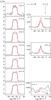 |
Fig. 4 Rotational lines of SiO in IRC +10216 as observed with the IRAM 30-m telescope (black histograms) and as calculated with the radiative transfer model (red lines). |
As shown in Fig. 3, there is a good overall agreement between calculated and observed line profiles for CS, except for the v = 1, J = 3−2 line whose observed intensity is substantially larger than calculated. This line is probably affected by a maser amplification, as indicated by the high spectral resolution observations made by Highberger et al. (2000). These authors point towards a mechanism based on infrared pumping to the v = 1 state, something that is included in our radiative transfer treatment, but does not produce a maser amplification in this line. A more likely mechanism for this relatively weak maser could be the overlap of ro-vibrational CS lines with those of abundant molecules such as SiO, a mechanism that explain the maser emission observed in oxygen-rich AGB stars in several rotational transitions of 29SiO and 30SiO, and of SiO in the v = 3 and v = 4 vibrational states (González-Alfonso & Cernicharo 1997), and in some SiS rotational lines within the ground vibrational state in IRC +10216 (Fonfría Expósito et al. 2006; see below).
The excitation of CS throughout the envelope is dominated by collision processes although the absorption of infrared photons emitted by the central star and by the warm dust also plays an important role. Radiative pumping at 8 μm populates the vibrationally excited states, enhancing the emission in lines such as the v = 3 J = 7−6 (whose levels lie 5500 K above the ground state and which otherwise would not be detectable), but also, through downward cascades, affects the population of the v = 0 rotational levels. Therefore, a proper treatment of infrared pumping warrants a correct estimation of the abundance in the inner layers (through the vibrationally excited lines) and allows also to accurately determine the abundance in the outer envelope, which would be overestimated by about 30% if IR pumping were neglected. According to our analysis, the abundance of CS relative to H2 is 4 × 10⁻⁶ in the inner layers and drops to 7 × 10⁻⁷ in the outer layers (see Fig. 12). The estimated uncertainty of the abundance is 50% in the outer envelope, and a factor of 2 for the regions inner to Rc, where densities are more uncertain. Figure 3 shows the improvement in the fit to the line profiles brought by the two abundance components model.
In the case of SiO, we have observed the J = 2−1 through J = 7−6 lines of the ground vibrational state as well as 3 lines of the v = 1 state. As shown in Fig. 4, there is a good agreement between calculated and observed line profiles. A slight difference is however found in the v = 0 line shapes (calculated are parabolic while observed have a slight double-peak character), which may be indicative of a more extended SiO envelope. A better agreement is found, rather than by extending SiO to larger radii, by enhancing its excitation in the outer layers. A possible source for the required additional excitation could be provided by shells with enhanced density, known to be present in the outer layers of IRC +10216 (see Mauron & Huggins 1999; Cordiner & Millar 2009; De Beck et al. 2012), or by an infrared pumping larger than given by our model. We have nevertheless not attempted to improve the agreement for SiO, which overall is satisfactory enough, by modifying the physical model, since this would affect all the other molecules. The excitation of SiO levels in the model is very similar to that found for CS, i.e., is controlled by inelastic collisions with H2 while radiative pumping at 8 μm affects the intensities of the v = 0 rotational lines by about 30% and completely dominates the excitation of the vibrationally excited states. The derived SiO abundance, 1.8 × 10⁻⁷ relative to H2, remains constant from the innermost layers up to the photodissociation region (see Fig. 12). The uncertainty in the abundance is estimated to be 50% in the outer layers, rising to a factor of 2 in the inner regions, which are sampled by just a few vibrationally excited lines and where densities are more uncertain.
 |
Fig. 5 Rotational lines of SiS in IRC +10216 as observed with the IRAM 30-m telescope (black histograms) and as calculated with the radiative transfer model (blue lines). |
Silicon monosulphide (SiS) has been observed in a large number of rotational lines covering the v = 0 through v = 5 vibrational states (see Fig. 5). The analysis of this molecule is complicated by the fact that some rotational lines within the ground vibrational state (concretely the J = 11−10, J = 14−13, and J = 15−14) show a profile with enhanced emission due to maser amplification at certain velocities, which are probably caused by the overlap at 13.5 μm of ro-vibrational transitions of SiS with those of C2H2 and HCN (Fonfría Expósito et al. 2006). The agreement between calculated and observed line profiles is somewhat poorer than in the cases of CS and SiO. On the one hand our radiative transfer calculations do not include infrared overlaps, something that clearly affects the three maser lines previously mentioned but can also have an influence on the excitation of other vibrationally excited lines (see Fonfría Expósito et al. 2006), and on the other hand the observed intensity of some high frequency lines may have non negligible errors due to calibration (estimated to be around 30% in the λ0.9 mm band), to pointing inaccuracies (which are typically < 2′′, although the main beam of the IRAM 30-m telescope is as small as 7′′ at 360 GHz and vibrationally excited lines have an emission size of less than 1′′), or even due to time variability (difficult to evaluate due to the lack of observations at different times in the λ0.9 mm band).
Infrared pumping affects little the level populations within the ground vibrational state of SiS, but controls, at practically the same extent than collisions, the excitation of the vibrationally excited lines. As in the case of CS, we need to increase the abundance of SiS in the inner layers with respect to that in the outer envelope. We derive for SiS an abundance relative to H2 of 3 × 10⁻⁶ in the inner layers, decreasing down to a value of 1.3 × 10⁻⁶ in the mid and outer layers (see Fig. 12). The estimated uncertainty in the abundance of SiS is a factor of 2 in the inner layers and 60% for the outer envelope.
 |
Fig. 6 Rotational lines of Na35Cl in IRC +10216 as observed with the IRAM 30-m telescope (black histograms) and as calculated with the radiative transfer model (green lines). Continuous lines refer to the best model, using the abundance profile shown in Fig. 13, while dashed lines result from a model without the abundance decrease in the 1 − 3 R∗ region. Note that dashed lines overestimate the intensity at the center of high-J lines. |
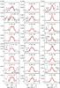 |
Fig. 7 Rotational lines of K35Cl in IRC +10216 as observed with the IRAM 30-m telescope (black histograms) and as calculated with the radiative transfer model (red lines). |
The metal halides NaCl, KCl, AlCl, and AlF are all observed through rotational transitions within the ground vibrational state. No vibrationally excited lines are detected, probably because of the low abundance of these species. The observed and calculated line profiles of Na35Cl and K35Cl are shown in Figs. 6 and 7, respectively. These two species have similar dipole moments, so that the larger intensity of the NaCl lines largely reflects its larger abundance with respect to KCl. The abundance derived for Na35Cl in the inner layers is 1.3 × 10⁻⁹ relative to H2 (with an uncertainty of a factor of 2), although we find necessary to decrease the abundance in the thermochemical equilibrium region (1 − 3 R∗) down to a value of 10-11 (see Fig. 13) to avoid a too strong emission for the high-J lines near the central velocity (see Fig. 6). In the case of K35Cl the derived abundance profile is somewhat more elaborated (see Fig. 13). KCl abundance is found to have a slight gradient going from 5 × 10⁻¹⁰ at 5 R∗ down to 3.7 × 10⁻¹⁰ in the outer layers, with an estimated error of a factor of 2. As with NaCl, the abundance is decreased in the 1−3 R∗ region, although in this case by just a factor of 2.5.
The observed and calculated line profiles of Al35Cl and AlF are shown in Figs. 8 and 9, respectively. AlCl and AlF have a much smaller dipole moment than NaCl, but show similar line intensities, which suggest they are fairly more abundant. Radiative transfer calculations confirm this point and yield abundances relative to H2 of 5 × 10⁻⁸ for Al35Cl and 10-8 for AlF (with an uncertainty of 50% increasing up to a factor of 2 in the regions inner to Rc). In the thermochemical equilibrium region (1−3 R∗) the abundance of Al35Cl is decreased, as for Na35Cl and K35Cl, by a factor of 5 (see Fig. 13). It is worth to note that the observed lines of AlF are slightly more U-shaped than those of AlCl. Such behavior can be accounted for to some extent by assuming that AlF is more extended than AlCl due to a lower photodissociation rate, as assumed in our model (see Sect. 4.2). Still the observed line profiles of AlF have a slightly more pronounced U-shape than calculated (see Fig. 9). Here, as occurs with SiO (see above), a better agreement cannot be obtained by extending AlF to larger radii, but by enhancing the excitation of AlF in the outer layers. In fact, assuming LTE excitation for AlF brings the calculated line profiles in close agreement with the observed ones. This is somewhat paradoxical since AlF is the only metal-bearing molecule for which collision rate coefficients have been calculated. This slight discrepancy is, nevertheless, unlikely to have a significant impact on the AlF derived abundance.
 |
Fig. 8 Rotational lines of Al35Cl in IRC +10216 as observed with the IRAM 30-m telescope (black histograms) and as calculated with the radiative transfer model (blue lines). |
The excitation of the metal halides in IRC +10216 is likely to be dominated by inelastic collisions. The role of infrared pumping to vibrationally excited levels, not included in our radiative transfer calculations, is difficult to evaluate mostly due to the lack of ro-vibrational line strengths. To get a rough idea of the importance of infrared pumping we have run radiative transfer models including the first vibrationally excited state. As dipole moment for the v = 1 → 0 band we have adopted that of SiS (0.13 D), scaled by the ratio of the halide to SiS permanent electric dipole moments. These calculations indicate that infrared pumping does not significantly affect the intensities of the observed lines, except for the high-J lines of NaCl which are slightly more intense with respect to the case when infrared pumping is not included. We may conclude that it is unlikely that infrared pumping plays an important role in the excitation of the v = 0 rotational levels of these metal halides, which is very likely dominated by collision processes.
Even in the absence of IR pumping, the ground vibrational state populations of metal halides depart from LTE, according to our statistical equilibrium calculations. Figure 10 shows, for selected rotational transitions, the calculated ratio of the excitation to kinetic temperature as a function of radius. We see that for the 4 metal halides this ratio is equal to 1 in the inner layers, i.e. the rotational levels are thermalized, whereas at larger radii the decrease in density makes rotational levels to be subthermally populated yielding excitation temperatures lower than the kinetic temperature. NaCl and KCl, with a large dipole moment, start to deviate from thermalization at radii much shorter than AlCl and AlF, which due to their moderately low dipole moments keep close to thermalization throughout a large part of the envelope. This suggests that the choice of the collision rate coefficients should not be critical for AlCl and AlF.
Finally, as concerns the cyanide NaCN, a fairly large number of rotational lines within the ground vibrational state has been observed (see Fig. 11). Although the agreement between calculated and observed line profiles is overall satisfactory, taking into account the large uncertainty of the collision rate coefficients, the calculated high-J high-Ka lines are too strong and the low-J and low-Ka lines too weak. We note that the discrepancy is larger if we replace statistical equilibrium calculations by LTE. The adopted photodissociation rate of NaCN is also very uncertain (see Sect. 4.2). Our model points toward a lower photodissociation rate than adopted, which would extend the NaCN envelope increasing the intensity of low-J lines, although this conclusion is hampered by the uncertain collision rates adopted, which are likely to cause most of the observed discrepancies. The role of infrared pumping to vibrationally excited states is difficult to evaluate due to the lack of spectroscopic and line strengths data for such states. The derived abundance for NaCN is 3 × 10⁻⁹ relative to H2, with an estimated uncertainty of a factor of 3. Decreasing the NaCN abundance in the 1 − 3 R∗ region, down to a very low value (10-12), improves somewhat the fit to the observed high-J high-Ka lines.
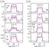 |
Fig. 9 Rotational lines of AlF in IRC +10216 as observed with the IRAM 30-m telescope (black histograms) and as calculated with the radiative transfer model (magenta lines). |
 |
Fig. 10 Calculated ratio of excitation temperature to kinetic temperature (Tex/Tk) as a function of radius for selected rotational transitions of the metal halides Na35Cl, K35Cl, Al35Cl, and AlF in IRC +10216. |
 |
Fig. 11 Rotational lines of NaCN in IRC +10216 as observed with the IRAM 30-m telescope (black histograms) and as calculated with the radiative transfer model (blue lines). Lines are ordered by increasing frequency from bottom to top (and from left to right). |
Molecular abundances in the inner layers of IRC +10216.
5. Discussion
5.1. Molecular abundances
 |
Fig. 12 Abundances of CS, SiO, and SiS in IRC +10216, as derived from the radiative transfer model (continuous lines) and as calculated through thermochemical equilibrium in the innermost regions of the envelope (dashed lines). A vertical dashed line indicates the outer boundary where thermochemical equilibrium is valid (~3 R∗). |
A compilation of molecular abundances for the inner layers of IRC +10216, resulting from this work and from previous studies, is given in Table 10. The abundance profiles derived in this study are shown in Fig. 12 for CS, SiO, and SiS, and in Fig. 13 for NaCl, KCl, AlCl, AlF, and NaCN. For chlorine-containing molecules, the abundances given in Table 10 and shown in Fig. 13 include both the 35Cl and 37Cl isotopic species, with a 35Cl/37Cl ratio of 2.9, as derived in Sect. 5.2.
In Figs. 12 and 13 we also show the abundances computed under thermochemical equilibrium, which is expected to be valid from the stellar photosphere up to a radius of ~3 R∗, from which the decrease in density and temperature causes an increase in the chemical time scale so that the abundances experience a quenching effect (see Agúndez & Cernicharo 2006). The thermochemical equilibrium calculations use solar elemental abundances (Asplund et al. 2009), except for carbon whose abundance is increased over the oxygen value by a factor of 1.5. More details on the thermochemical equilibrium calculations can be found in Agúndez (2009). By looking at Figs. 12 and 13, we note that for most of the studied molecules – a notable exception is CS – the abundance calculated under thermochemical equilibrium shows a positive gradient in the 1−3 R∗ region, i.e. the abundance close to the photosphere is much lower than in the surroundings of the quenching region (~3 R∗). This behavior justifies the decrease in abundance in the 1−3 R∗ region adopted for various metal-bearing molecules.
For some species (CS, SiS, and KCl) we have found necessary to consider a negative gradient in the abundance, with a higher value in the inner layers than in the mid and outer regions, in order to adequately reproduce the wide range of low- and high-energy observed transitions. The scientific rationale for such a gradient is that the studied molecules contain refractory elements and are likely to deplete from the gas phase to condense onto dust grains. Therefore, we consider that the gradient starts at the condensation radius Rc and continues up to a radius of a few 1015 cm. Farther out, at about 1016 cm all molecules start to be photodissociated by the ambient interstellar ultraviolet field. The observation of a large number of rotational lines for the different molecules studied, involving levels with a wide range of energies (including highly excited vibrational levels) allows us to trace the material, and therefore to determine the abundance, from the innermost layers out to the outer envelope.
Carbon monosulphide (CS) is found to have an abundance relative to H2 of 4 × 10⁻⁶ in the inner layers, decreasing in the mid envelope down to a value of 7 × 10⁻⁷ at a radius of 2 × 1015 cm, which serves as input value for the photochemistry taking place in the outer envelope (see Fig. 12). Our estimate for the inner layers may be compared with the results of the thermochemical equilibrium calculations, which yield a steep abundance gradient around the quenching region, from 2 × 10⁻⁵ at 2 R∗ down to 3 × 10-11 at 4 R∗. The intersection of our derived abundance profile with that calculated under thermochemical equilibrium indicates that the abundance of CS is quenched at a radius of 2.4 R∗. The model built by Willacy & Cherchneff (1998), which considers the effect of shocks induced by the stellar pulsation on the chemistry, predicts abundances somewhat lower in the inner layers, 2−6 × 10⁻⁷ in the 2.7 − 5 R∗ region. Our findings for the inner layers are in perfect agreement with the previous results of Keady & Ridgway (1993), who derive an abundance of 4 × 10⁻⁶ for the region inner to 17 R∗ from observations of ro-vibrational lines in the infrared, but differ significantly from the estimates made by Highberger et al. (2000), 3 − 7 × 10⁻⁵ at 14 R∗, and by Patel et al. (2009), > 9.3 × 10⁻⁶ within a radius of 7 R∗, which are based on observations of rotational lines in vibrationally excited states and an analysis involving column densities and mean excitation temperatures. As concerns the abundance in the mid and outer envelope, our estimate, 7 × 10⁻⁷, is somewhat higher than the previous value derived by Henkel et al. (1985), 1.2 × 10⁻⁷, based on the observation of low-J rotational lines within the ground vibrational state.
 |
Fig. 13 Abundances of NaCl, KCl, AlCl (including 35Cl and 37Cl), AlF, and NaCN in IRC +10216, as derived from the radiative transfer model (continuous lines) and as calculated through thermochemical equilibrium in the innermost regions of the envelope (dashed lines). A vertical dashed line indicates the outer boundary where thermochemical equilibrium is valid (~3 R∗). |
For silicon monoxide (SiO) we derive an abundance relative to H2 of 1.8 × 10⁻⁷, from the innermost circumstellar layers up to the photodissociation region. Yet, as in the case of CS, chemical equilibrium calculations (see Fig. 12) yield a steep gradient near the quenching region, with a value as low as 3 × 10⁻¹⁰ at 2 R∗ increasing up to 10-6 at 4 R∗. The quenching radius for SiO would be located around 3.6 R∗, somewhat farther than that of CS. We find no evidence of such a low SiO abundance in the innermost layers, perhaps because only a few vibrationally excited lines tracing this region enter in our analysis. Calculations based on chemical kinetics (see model MH in Fig. 3 of Agúndez & Cernicharo 2006) indicate that the abundance of SiO increases when moving away from the photosphere due to the reaction between Si and CO, which after a few stellar radii becomes too slow compared to the dynamical time scale, so that the abundance of SiO gets quenched. The chemical model with shocks of Willacy & Cherchneff (1998) predicts an abundance of 2−7 × 10⁻⁷ in the 1.9−5 R∗ region, which is in good agreement with our derived value.
As concerns previous observational studies, one of the most complete dealing with the abundance of SiO in IRC +10216 is that made by Schöier et al. (2006a), who used observations of several rotational lines within the ground vibrational state, interferometric observations of the v = 0 J = 5−4 line, as well as ro-vibrational lines observed at 8 μm to derive the abundance of SiO throughout the envelope. They found an abundance of 3 × 10⁻⁸ from the photosphere up to 1.7 × 1014 cm, a high abundance component of 1.5 × 10⁻⁶ extending up to 4.5 × 1014 cm (which is necessary to reproduce the ro-vibrational lines observed), and an abundance of 1.7 × 10⁻⁷ from this latter radius up to the outer layers. The main difference with our results is that Schöier et al. (2006a) find necessary to adopt a high abundance component in the inner layers. A higher abundance than derived by us, 8 × 10⁻⁷, was also found by Keady & Ridgway (1993) in their analysis of the observations at 8 μm. These authors adopt lower densities than us for the inner layers, they assume that Eq. (3) applies down to the photosphere, and this could explain the higher abundances they get. On the other hand, the abundance derived by Keady & Ridgway (1993) for CS is in very good agreement with our value (see above), in spite of the very different densities adopted for the inner regions. Given the different nature of the lines used to trace the abundance in the inner layers, infrared ro-vibrational lines versus millimeter rotational lines in vibrationally excited states, it is difficult to explain why the abundances found by Keady & Ridgway (1993) and by us are different for SiO but not for CS. A forthcoming study of new high spectral resolution observations (R ~ 100 000) of IRC +10216 around 8 μm obtained from ground (Fonfría et al., in prep.) will help to solve the discrepancy found between our derived SiO abundance and that found by Keady & Ridgway (1993).
More recently, Decin et al. (2010a) have observed a large number of SiO rotational transitions in IRC +10216, some of them in the v = 1 state, at low spectral resolution with the SPIRE and PACS instruments on board Herschel. These authors derive an abundance of 10-7 for SiO from the innermost regions up to the outer layers, in good agreement with our findings.
According to our best model, silicon monosulphide (SiS) is present in the inner layers with an abundance relative to H2 of 3 × 10⁻⁶, decreasing in the mid envelope down to a value of 1.3 × 10⁻⁶ at a radius of 2 × 1015 cm. As shown in Fig. 12, the thermochemical equilibrium abundance of SiS shows a steep gradient, rising from 10-7 at the photosphere up to a maximum value of 2.6 × 10⁻⁵ beyond 2.5 R∗. Our derived abundance is substantially lower than this latter value, which points towards the SiS abundance being quenched in a region inner to 2.5 R∗, concretely at 1.9 R∗, as deduced from the intersection of the continuous and dashed lines in Fig. 12. Calculations based on chemical kinetics (Willacy & Cherchneff 1998; Agúndez & Cernicharo 2006) result in SiS abundances of 2 − 3 × 10⁻⁵ in the regions inner to 5 R∗, about one order of magnitude larger than the value we find. These models are, however, affected by uncertainties due to the poor knowledge of rate constants for reactions involving Si- and S-bearing species.
As concerns previous observational studies, there is a general consensus on the presence of a gradient in the abundance of SiS, with reported values in the range 10-6 − 10-5 in the inner layers (>6.5 × 10⁻⁷ by Turner 1987; 7.5 × 10⁻⁶ by Bieging & Nguyen-Q-Rieu 1989; 4.3 × 10⁻⁵ close to the stellar surface decreasing down to 4.3 × 10⁻⁶ at 12 R∗ by Boyle et al. 1994) and reported values in the range 10-7 − 10-6 in the outer envelope (2.4 × 10⁻⁷ by Sahai et al. 1984; 5 × 10⁻⁷ by Nguyen-Q-Rieu et al. 1984; 5 × 10⁻⁷ by Henkel et al. 1983; 1.5 − 4 × 10⁻⁷ by Henkel et al. 1985; 6.5 × 10⁻⁷ by Bieging & Nguyen-Q-Rieu 1989; 1.4 × 10⁻⁶ by Schöier et al. 2007). The more recent study of Decin et al. (2010a), based on observations with SPIRE and PACS that are particularly sensitive to the warm inner envelope, reports a SiS abundance of 4 × 10⁻⁶, in good agreement with our finding for the inner layers.
The most abundant sulfur-bearing molecules in IRC +10216 are therefore CS and SiS, H2S being a minor species (see Table 10). Assuming a solar elemental abundance, we conclude that 27% of the total available sulfur is locked in gas phase CS and SiS molecules in the inner layers. The fraction decreases down to 7.6% in the outer envelope, an evidence of sulfur depletion onto dust grains in the dust formation region. A fraction of the remaining sulfur could be in atomic form, but it is likely that the bulk of sulfur is in the form of solid condensates such as MgS (Goebel & Moseley 1985). Several silicon-bearing molecules such as SiS, SiO, SiC2, and SiH4 are present in the inner envelope, all them locking up to 5.6% of the total available silicon. This small fraction, together with the fact that SiS (the most abundant Si-containing molecule) gets depleted by a factor of 2.3 after the dust condensation region, indicates that silicon massively condenses into dust grains, mainly forming SiC (Treffers & Cohen 1974). We see no evidence of SiO depletion at the dust formation region in our SiO abundance profile. One would expect a depletion similar to that of SiS, silicon being a refractory element that is thought to easily condense onto dust grains in the envelopes of AGB stars (Schöier et al. 2006b). This may result from our small sample of vibrationally excited SiO lines, which limits our sensitivity to the innermost layers.
The metal halides NaCl, KCl, AlCl, and AlF, and the cyanide NaCN are among the first metal-containing molecules detected in space (Cernicharo & Guélin 1987; Turner et al. 1994). Metal-bearing molecules are rarely observed in the gas phase of the interstellar medium due to their large refractory character that make them to easily form solid condensates. Their presence in IRC +10216 is largely caused by the high temperatures and densities prevailing close to the star, where, under thermochemical equilibrium, a good fraction of metals are in the gas phase forming this kind of molecules.
The derived abundances relative to H2 in the inner layers are 1.8 × 10⁻⁹ for NaCl, 7 × 10⁻¹⁰ for KCl, 7 × 10⁻⁸ for AlCl, 10-8 for AlF, and 3 × 10⁻⁹ for NaCN. For some of these molecules the abundance has been decreased in the 1 − 3 R∗ region, in order to better account for the observed line profiles. The rationale for this abundance modification is related to the thermochemical equilibrium calculations, which for all these species show a strong abundance gradient in this region, with low values close to the stellar surface and higher values around the quenching region (see Fig. 13). For NaCl and KCl, the abundance decrease in this 1 − 3 R∗ region improves significantly the agreement between calculated and observed line profiles, indicating that these species are likely depleted close to the photosphere by at least a factor of ~ 100 for NaCl and ~ 2 − 3 for KCl. For AlCl and NaCN, the abundance decrease adopted in the 1 − 3 R∗ region affects only slightly the profiles of the observed lines, while for AlF no abundance modification has been adopted since line profiles are almost not affected. The observed lines of AlCl, AlF, and NaCN are therefore not sensitive enough to the abundance in this innermost region, and it cannot be excluded that these molecules have an abundance as low as predicted by TE close to the star. Vibrationally excited lines should allow to better probe this region.
The abundances calculated under thermochemical equilibrium are in reasonable agreement with our derived values, although some remarks should be made. For the metal chlorides NaCl and KCl, the derived abundances are higher by about one order of magnitude than the maximum values given by thermochemical equilibrium in the surroundings of the quenching region (see Fig. 13), something that could be indicative of non-equilibrium processes being at work to enhance the abundances of NaCl and KCl. In the case of AlCl and AlF, the derived abundances are in good agreement with the thermochemical equilibrium calculations, pointing towards the abundance of these two molecules being quenched at a radius of 2.6 R∗. For NaCN, the analysis is not so obvious as the abundance calculated under thermochemical equilibrium shows a steep positive gradient that reaches the derived abundance of 3 × 10⁻⁹ at a radius of ~ 6 R∗, somewhat farther than the typical quenching region located around 3 R∗. The lack of chemical kinetics data on reactions involving NaCN makes it difficult to evaluate whether such a large quenching radius is still possible or not.
Metals are refractory elements, so that we expect metal-containing molecules to deplete from the gas phase to incorporate into dust grains in the condensation region. Surprisingly, we find no evidence for such depletion except for KCl, whose abundance is found to slightly decrease from its value of 5 × 10⁻¹⁰ in the inner layers down to 3.7 × 10⁻¹⁰ at a radius of 2 × 1015 cm. It therefore seems that the presence of metals in the gas phase is not just restricted to the warm inner circumstellar regions, but also to the cool outer regions where a non negligible fraction survives in the gas phase. Further evidence to this respect comes from the observation of other metal-bearing molecules in the outer layers of IRC +10216, such as MgNC (Guélin et al. 1993), MgCN (Ziurys et al. 1995), AlNC (Ziurys et al. 2002) KCN (Pulliam et al. 2010), and FeCN (Zack et al. 2011), and from the remarkable detection of gas phase atomic metals in the outer envelope of IRC +10216 by Mauron & Huggins (2010). As already pointed out by these latter authors, metals must be mostly in solid state in the outer layers of IRC +10216 since gas phase species do only account for a relatively small fraction of the total available elemental abundance, 24% as NaI and NaII and 0.14% as NaCl and NaCN in the case of sodium, 5% as KI and KII and 0.5% as KCl and KCN as concerns potassium, and 1.4% as AlCl, AlF, and AlNC in the case of aluminium. These small percentages are however remarkable, given the low temperatures prevailing in the outer layers, and are high enough to allow for a metal-based gas phase chemistry to take place. In the inner layers the situation should not be very different, as inferred from the derived molecular abundances, with metals being mostly in the form of solid condensates (only beyond the condensation radius) and gas phase atoms, and a small but sizable fraction being locked in gas phase molecules.
5.2. Isotopic ratios
For some of the studied molecules, a good number of transitions of rare isotopomers have been observed (see Tables 1 − 6), allowing us to determine the corresponding isotopic abundance ratios. For each of these rare isotopomers we have adopted the abundance profile derived for the main isotopomer, decreased by the corresponding isotopic ratio, which is varied until the line profiles calculated with the radiative transfer model reproduce the observed ones. As compared with the previous method used to derive isotopic ratios from line intensity ratios (e.g. Cernicharo et al. 2000; Kahane et al. 2000), the method used here, based on LVG radiative transfer calculations, can better, although not completely, deal with optical depth effects present in the lines of some main isotopomers. Such effects can be completely avoided by using optically thin lines of doubly substituted isotopic species, but such lines are weak and are observed with low signal-to-noise ratios, which may introduce large uncertainties in the derived isotopic ratios. Here, we have therefore focused on single substituted isotopomers.
Isotopic ratios in IRC +10216.
The derived isotopic ratios are given in Table 11. Under the reasonable assumption of a similar excitation and spatial extent for two isotopomers, most of the errors that usually affect the determination of an abundance, cancel when deriving an isotopic ratio (see Kahane et al. 2000). The estimated uncertainties given in Table 11, therefore, neglect any error coming from the model and are simply based on the signal-to-noise ratio of the observed lines (of main and rare isotopomers), and on the sensitivity of the calculated line profiles to the adopted isotopic ratio.
We find an elemental 12C/13C ratio of 35 ± 3.5 from the observed lines of 12CS and 13CS (see Table 1), somewhat lower than the value of 45 ± 3 derived from intensity ratios of optically thin lines of SiC2 and CS (Cernicharo et al. 2000). In the case of the sulfur isotope 32S, we derive values of C32S/C34S = 16 ± 2.5 and Si32S/Si34S = 22 ± 2.5. The different values should result, rather than from 32S isotopic fractionation which is unlikely in warm regions, from optical depth effects that are more important for CS than for SiS. We thus adopt the Si32S/Si34S isotopic ratio as a better proxy of the elemental 32S/34S abundance ratio. A similar situation is found for the sulfur isotope 33S, for which we derive C32S/C33S = 83 ± 11 and Si32S/Si33S = 112 ± 12, the latter value being a better estimation of the elemental 32S/33S. The isotopic ratios found for carbon and sulfur are similar or slightly smaller than those previously derived by Cernicharo et al. (2000) from intensity ratios of optically thin lines. The fact that the 12C/13C and 32S/33S ratios derived here are somewhat smaller than those found by Cernicharo et al. (2000) probably indicates that our results are affected to some extent by optical depth effects. The usefulness of the method utilized here is clear in cases where optically thin lines (e.g. of doubly substituted isotopomers) are close or below the detection limit of the observations. This occurs in the cases of the 28Si/29Si and 28Si/30Si ratios, for which we find values (see Table 11) consistent with the lower limits given by Cernicharo et al. (2000).
The 35Cl/37Cl isotopic ratio is found to be 2.9 ± 0.3 from the lines of NaCl, KCl, and AlCl, which is in between the value of 2.3 ± 0.24 found by Kahane et al. (2000) from intensity ratios of some lines of NaCl and AlCl, and the value of 3.3 ± 0.3 derived by Agúndez et al. (2011) from the modeling of the J = 1 − 0 to J = 3 − 2 lines of HCl. The low 35Cl/37Cl ratio found by Kahane et al. (2000) indicates that lines of NaCl and AlCl could be affected by optical depth effects, so that their calculated value based on line intensity ratios would be a lower limit to the true isotopic ratio. Finally, as concerns the 16O/17O and 16O/18O ratios, we have not attempted to determine them due to the low signal-to-noise ratios of the observed Si17O and Si18O lines (see Table 2). We nevertheless find that the observed lines of these two rare isotopomers are consistent with the oxygen isotopic ratios 16O/17O = 840 and 16O/18O = 1260 given by Kahane et al. (2000).
The isotopic ratios derived here, although systematically smaller, are very close to the solar values, to the exception of 12C/13C (see Table 11). Since a bias towards smaller ratios is expected, due to the residual optical depth effects, we conclude that the elemental isotopic ratios 32S/34S, 32S/33S, 28Si/29Si, 28Si/30Si, and 35Cl/37Cl in IRC +10216 are compatible with the solar values. This result is not unexpected since the central AGB star is not massive enough to form much S, Si, or Cl. The lower 12C/13C ratio found in IRC +10216, as compared with that in the Sun, is known to result from CNO cycle nuclear processing in the interior of the star (Kahane et al. 2000).
6. Summary
Astronomical observations of the carbon star envelope IRC +10216 extending over the full frequency coverage of the IRAM 30-m telescope (80 − 357.5 GHz) have been analyzed to obtain accurate abundances for several molecules formed in the inner layers: CS, SiO, and SiS, the metal halides NaCl, KCl, AlCl, and AlF, and the metal cyanide NaCN. The observation of a large number of rotational transitions covering a wide range of energy levels, including highly excited vibrational states, allow us to derive abundances from the innermost layers out to the outer regions where molecules are photodissociated by interstellar ultraviolet photons. For some molecules, noticeably CS and SiS, we find that abundances are depleted from the inner to the outer layers, implying that they contribute to the formation of dust. The amount of sulfur and silicon locked up in gas phase molecules in the inner layers, 27% and 5.6% respectively, indicates that a major fraction of these elements is in the form of solid condensates, most likely as MgS and SiC, in IRC +10216’s envelope. Metal-bearing molecules lock a relatively small fraction (a few percent) of metals. Nevertheless, we find that NaCl, KCl, AlCl, AlF, and NaCN, which all contain refractory elements, seem to maintain a surprisingly high abundance in the cold outer layers, where they can participate, together with metallic atoms, in a rich gas phase chemistry. The lines of rare isotopomers of CS, SiO, SiS, and some metal compounds have been analyzed, and we derive abundance ratios for rare isotopes of carbon, sulfur, silicon, and chlorine. The values obtained are in good agreement with previously reported values. They are consistent with the solar values, except for the 12C/13C ratio, which is more than twice smaller in IRC +10216 than in the Sun, in agreement with previous findings.
Online material
CS line parameters in IRC +10216.
SiO line parameters in IRC +10216.
SiS line parameters in IRC +10216.
NaCl line parameters in IRC +10216.
KCl line parameters in IRC +10216.
AlCl line parameters in IRC +10216.
AlF line parameters in IRC +10216.
NaCN line parameters in IRC +10216.
Acknowledgments
We acknowledge the referee, H. Olofsson, for a constructive report. M.A., J.C., and F.D. thank the Spanish MICINN for funding support through the grant AYA2009-07304 and the ASTROMOL Consolider project CSD2009-00038. During this study M.A. has been supported by Spanish MEC grant AP2003-4619, Spanish MICINN projects PIE 200750I024 and PIE 200750I028, Marie Curie Intra-European Individual Fellowship 235753, and ERC project 209622 E3ARTHs. J.P.F. has been supported by the UNAM through a postdoctoral fellowship.
References
- Agúndez, M. 2009, Ph.D. Thesis, Universidad Autónoma de Madrid [Google Scholar]
- Agúndez, M., & Cernicharo, J. 2006, ApJ, 650, 374 [NASA ADS] [CrossRef] [Google Scholar]
- Agúndez, M., Cernicharo, J., & Guélin, M. 2007, ApJ, 662, L91 [NASA ADS] [CrossRef] [Google Scholar]
- Agúndez, M., Cernicharo, J., Pardo, J. R., et al. 2008, A&A, 485, L33 [NASA ADS] [CrossRef] [EDP Sciences] [Google Scholar]
- Agúndez, M., Cernicharo, J., & Guélin, M. 2010, ApJ, 724, L133 [NASA ADS] [CrossRef] [Google Scholar]
- Agúndez, M., Cernicharo, J., Waters, L. B. F. M., et al. 2011, A&A, 533, L6 [NASA ADS] [CrossRef] [EDP Sciences] [Google Scholar]
- Asplund, M., Grevesse, N., Sauval, A. J., & Scott, P. 2009, ARA&A, 47, 481 [NASA ADS] [CrossRef] [Google Scholar]
- Bieging, J. H., & Nguyen-Q-Rieu 1989, ApJ, 343, L25 [NASA ADS] [CrossRef] [Google Scholar]
- Boyle, R. J., Keady, J. J., Jennings, D. E., Hirsch, K. L., & Wiedemann, G. R. 1994, ApJ, 420, 863 [NASA ADS] [CrossRef] [Google Scholar]
- Caris, M. 2004, J. Mol. Struct., 695, 243 [NASA ADS] [CrossRef] [Google Scholar]
- Caris, M., Lewen, F., & Winnewisser, G. 2002, Z. Naturforsch., 57a, 663 [Google Scholar]
- Castor, J. I. 1970, MNRAS, 149, 111 [NASA ADS] [Google Scholar]
- Cernicharo, J., & Guélin, M. 1987, A&A, 183, L10 [NASA ADS] [Google Scholar]
- Cernicharo, J., Barlow, M. J., González-Alfonso, E., et al. 1996, A&A, 315, L201 [NASA ADS] [Google Scholar]
- Cernicharo, J., Yamamura, I., González-Alfonso, E., et al. 1999, ApJ, 526, L41 [NASA ADS] [CrossRef] [PubMed] [Google Scholar]
- Cernicharo, J., Guélin, M., & Kahane, C. 2000, A&AS, 142, 181 [NASA ADS] [CrossRef] [EDP Sciences] [Google Scholar]
- Cernicharo, J., Waters, L. B. F. M., Decin, L., et al. 2010, A&A, 521, L8 [NASA ADS] [CrossRef] [EDP Sciences] [Google Scholar]
- Cernicharo, J., Agúndez, M., Kahane, C., et al. 2011, A&A, 529, L3 [NASA ADS] [CrossRef] [EDP Sciences] [Google Scholar]
- Chandra, S., Kegel, W. H., Le Roy, R. J., & Hertenstein, T. 1995, A&AS, 114, 175 [NASA ADS] [Google Scholar]
- Cherchneff, I. 2006, A&A, 456, 1001 [NASA ADS] [CrossRef] [EDP Sciences] [Google Scholar]
- Cherchneff, I., Barker, J. R., & Tielens, A. G. G. M. 1992, ApJ, 401, 269 [NASA ADS] [CrossRef] [Google Scholar]
- Cordiner, M. A., & Millar, T. J. 2009, ApJ, 697, 68 [NASA ADS] [CrossRef] [Google Scholar]
- Crosas, M., & Menten, K. M. 1997, ApJ, 483, 913 [NASA ADS] [CrossRef] [Google Scholar]
- Daniel, F., & Cernicharo, J. 2008, A&A, 488, 1237 [NASA ADS] [CrossRef] [EDP Sciences] [Google Scholar]
- Dayou, F., & Balança, C. 2006, A&A, 459, 297 [NASA ADS] [CrossRef] [EDP Sciences] [Google Scholar]
- De Beck, E., Lombaert, R., Agúndez, M., et al. 2012, A&A, 539, A108 [NASA ADS] [CrossRef] [EDP Sciences] [Google Scholar]
- De Leeuw, F. H., van Wachen, R., & Dymanus, A. 1970, J. Chem. Phys., 53, 981 [NASA ADS] [CrossRef] [Google Scholar]
- Decin, L., Cernicharo, J., Barlow, M. J., et al. 2010a, A&A, 518, L143 [NASA ADS] [CrossRef] [EDP Sciences] [Google Scholar]
- Decin, L., Agúndez, M., Barlow, M. J., et al. 2010b, Nature, 467, 64 [NASA ADS] [CrossRef] [PubMed] [Google Scholar]
- Draine, B. T. 1978, ApJS, 36, 595 [NASA ADS] [CrossRef] [Google Scholar]
- Drira, I., Huré, J. M., Spielfiedel, A., Feautrier, N., & Roueff, E. 1997, A&A, 319, 720 [NASA ADS] [Google Scholar]
- Fonfría Espósito, J. P., Agúndez, M., Tercero, B., et al. 2006, ApJ, 646, L127 [NASA ADS] [CrossRef] [Google Scholar]
- Fonfría, J. P., Cernicharo, J., Ritcher, M. J., & Lacy, J. H. 2008, ApJ, 673, 445 [NASA ADS] [CrossRef] [Google Scholar]
- Glassgold, A. E. 1996, ARA&A, 34, 241 [NASA ADS] [CrossRef] [Google Scholar]
- Goebel, J. H., & Moseley, S. H. 1985, ApJ, 290, L35 [NASA ADS] [CrossRef] [Google Scholar]
- Goldflam, R., Green, S., & Kouri, D. J. 1977, J. Chem. Phys., 67, 4149 [NASA ADS] [CrossRef] [Google Scholar]
- Goldhaber, D. M., Betz, A. L., & Ottusch, J. J. 1987, ApJ, 314, 356 [NASA ADS] [CrossRef] [Google Scholar]
- González-Alfonso, E., & Cernicharo, J. 1997, A&A, 322, 938 [NASA ADS] [Google Scholar]
- Gotoum, N., Nkem, C., Hammami, K., et al. 2011, Ap&SS, 332, 209 [NASA ADS] [CrossRef] [Google Scholar]
- Gotoum, N., Hammami, K., Owono Owono, L. C., & Jaidane, N.-E. 2012, Ap&SS, 337, 553 [NASA ADS] [CrossRef] [Google Scholar]
- Green, S. 1995, ApJS, 100, 213 [NASA ADS] [CrossRef] [Google Scholar]
- Guélin, M., Lucas, R., & Cernicharo, J. 1993, A&A, 280, L19 [NASA ADS] [Google Scholar]
- Guélin, M., Lucas, R., & Neri, R. 1997, in CO: Twenty-Five Years of Millimeter Wave Spectroscopy, ed. W. B. Latter et al. (Dordrecht: Kluwer), IAU Symp., 170, 359 [Google Scholar]
- Halfen, D. T., & Ziurys, L. M. 2011, ApJ, 730, 107 [NASA ADS] [CrossRef] [Google Scholar]
- Hammami, K., Lique, F., Jaïdane, N., et al. 2007, A&A, 462, 789 [NASA ADS] [CrossRef] [EDP Sciences] [Google Scholar]
- Hasegawa, T. I., Kwok, S., Koning, N., et al. 2006, ApJ, 637, 791 [NASA ADS] [CrossRef] [Google Scholar]
- Hedderich, H. G., & Bernath, P. F. 1992, J. Mol. Spectr., 153, 73 [NASA ADS] [CrossRef] [Google Scholar]
- Hedderich, H. G., Dulick, M., & Bernath, P. F. 1993, J. Chem. Phys., 99, 8363 [NASA ADS] [CrossRef] [Google Scholar]
- Henkel, C., Matthews, H. E., & Morris, M. 1983, ApJ, 267, 184 [NASA ADS] [CrossRef] [Google Scholar]
- Henkel, C., Matthews, H. E., Morris, M., et al. 1985, A&A, 147, 143 [NASA ADS] [Google Scholar]
- Highberger, J. L., Apponi, A. J., Bieging, J. H., et al. 2000, ApJ, 544, 881 [NASA ADS] [CrossRef] [Google Scholar]
- Kahane, C., Dufour, E., Busso, M., et al. 2000, A&A, 357, 669 [NASA ADS] [Google Scholar]
- Keady, J. J., & Ridgway, S. T. 1993, ApJ, 406, 199 [NASA ADS] [CrossRef] [Google Scholar]
- Keady, J. J., Hall, D. N. B., & Ridgway, S. T. 1988, ApJ, 326, 832 [NASA ADS] [CrossRef] [Google Scholar]
- Kłos, J., & Lique, F. 2008, MNRAS, 390, 239 [NASA ADS] [CrossRef] [Google Scholar]
- Le Bertre, T. 1992, A&AS, 94, 377 [NASA ADS] [Google Scholar]
- Lide, D. R. 1965, J. Chem. Phys., 42, 1013 [NASA ADS] [CrossRef] [Google Scholar]
- Lique, F., & Spielfiedel, A. 2007, A&A, 462, 1179 [NASA ADS] [CrossRef] [EDP Sciences] [Google Scholar]
- Lique, F., Spielfiedel, A., & Cernicharo, J. 2006, A&A, 451, 1125 [NASA ADS] [CrossRef] [EDP Sciences] [Google Scholar]
- López Piñeiro, A., & Tipping, R. H. 1987, J. Mol. Spectr., 125, 91 [NASA ADS] [CrossRef] [Google Scholar]
- López Piñeiro, A., Tipping, R. H., & Chackerian, C. 1987, J. Mol. Spectr., 125, 184 [CrossRef] [Google Scholar]
- Lucas, R., Guélin, M., Kahane, C., et al. 1995, Ap&SS, 224, 293 [NASA ADS] [CrossRef] [Google Scholar]
- Mauron, N., & Huggins, P. J. 1999, A&A, 349, 203 [NASA ADS] [Google Scholar]
- Mauron, N., & Huggins, P. J. 2010, A&A, 513, A31 [NASA ADS] [CrossRef] [EDP Sciences] [Google Scholar]
- Men’shchikov, A. B., Balega, Y., Blöker, T., Osterbart, R., & Weigelt, G. 2001, A&A, 368, 497 [NASA ADS] [CrossRef] [EDP Sciences] [Google Scholar]
- Millar, T. J., Herbst, E., & Bettens, R. P. A. 2000, A&A, 316, 195 [Google Scholar]
- Monnier, J. D., Danchi, W. C., Hale, D. S., et al. 2000, ApJ, 543, 861 [Google Scholar]
- Morris, M. 1975, ApJ, 197, 603 [NASA ADS] [CrossRef] [Google Scholar]
- Müller, H. S. P., Schlöder, F., Stutzki, J., & Winnewisser, G. 2005, J. Mol. Struct., 742, 215 [NASA ADS] [CrossRef] [Google Scholar]
- Müller, H. S. P., McCarthy, M. C., Bizzocchi, L., et al. 2007, Phys. Chem. Chem. Phys., 9, 1579 [CrossRef] [PubMed] [Google Scholar]
- Nguyen-Q-Rieu, Bujarrabal, V., Olofsson, H., Johansson, L. E. B., & Turner, B. E. 1984, ApJ, 286, 276 [NASA ADS] [CrossRef] [Google Scholar]
- Patel, N. A., Young, K. H., Brünken, S., et al. 2009, ApJ, 692, 1205 [NASA ADS] [CrossRef] [Google Scholar]
- Patel, N. A., Young, K. H., Gottlieb, C. A., et al. 2011, ApJS, 193, 17 [NASA ADS] [CrossRef] [Google Scholar]
- Pulliam, R. L., Savage, C., Agúndez, M., et al. 2010, ApJ, 725, L181 [NASA ADS] [CrossRef] [Google Scholar]
- Raymonda, J. W., Muenter, J. S., & Klemperer, W. A. 1970, J. Chem. Phys., 52, 3458 [NASA ADS] [CrossRef] [Google Scholar]
- Ridgway, S. T., & Keady, J. J. 1988, ApJ, 326, 843 [NASA ADS] [CrossRef] [Google Scholar]
- Sahai, R., Wootten, A., & Clegg, R. E. S. 1984, ApJ, 284, 144 [NASA ADS] [CrossRef] [Google Scholar]
- Sanz, M. E., McCarthy, M. C., & Thaddeus, P. 2003, J. Chem. Phys., 119, 11715 [NASA ADS] [CrossRef] [Google Scholar]
- Schöier, F. L., Fong, D., Olofsson, H., et al. 2006a, ApJ, 649, 965 [NASA ADS] [CrossRef] [Google Scholar]
- Schöier, F. L., Olofsson, H., & Lundgren, A. A. 2006b, A&A, 454, 247 [NASA ADS] [CrossRef] [EDP Sciences] [Google Scholar]
- Schöier, F. L., Bast, J., Olofsson, H., & Lindqvist, M. 2007, A&A, 473, 871 [NASA ADS] [CrossRef] [EDP Sciences] [Google Scholar]
- Skinner, C. J., Justannont, K., Tielens, A. G. G. M., et al. 1999, MNRAS, 302, 293 [NASA ADS] [CrossRef] [Google Scholar]
- Suh, K.-W. 2000, MNRAS, 315, 740 [NASA ADS] [CrossRef] [Google Scholar]
- Tipping, R. H., & Chackerian, C. 1981, J. Mol. Spectr., 88, 352 [Google Scholar]
- Toboła, R., Lique, F., Kłos, J., & Chałasinski, G. 2008, J. Phys. B: At. Mol. Opt. Phys., 41, 155702 [NASA ADS] [CrossRef] [Google Scholar]
- Treffers, R., & Cohen, M. 1974, ApJ, 188, 545 [NASA ADS] [CrossRef] [Google Scholar]
- Turner, B. E. 1987, A&A, 183, L23 [NASA ADS] [Google Scholar]
- Turner, B. E., Steimle, T. C., & Meerts, L. 1994, ApJ, 426, L97 [NASA ADS] [CrossRef] [Google Scholar]
- van Dishoeck, E. W. 1998, in Rate Coefficients in Astrochemistry, ed. T. Millar, & D. Williams (Dordrecht: Kluwer), 49 [Google Scholar]
- van Dishoeck, E. W., Jonkheid, B., & van Hemert, M. C. 2006, Faraday Discuss., 133, 231 [Google Scholar]
- van Wachen, R., & Dymanus, A. 1967, J. Chem. Phys., 46, 3749 [NASA ADS] [CrossRef] [Google Scholar]
- Vincent, L. F. M., Spielfiedel, A., & Lique, F. 2007, A&A, 472, 1037 [NASA ADS] [CrossRef] [EDP Sciences] [Google Scholar]
- Willacy, K., & Cherchneff, I. 1998, A&A, 330, 676 [NASA ADS] [Google Scholar]
- Winnewisser, G., & Cook, R. L. 1968, J. Mol. Spectr., 28, 266 [NASA ADS] [CrossRef] [Google Scholar]
- Winters, J. M., Dominik, C., & Sedlmayr, E. 1994, A&A, 288, 255 [NASA ADS] [Google Scholar]
- Zack, L. N., Halfen, D. T., & Ziurys, L. M. 2011, ApJ, 733, L36 [NASA ADS] [CrossRef] [Google Scholar]
- Ziurys, L. M., Apponi, A. J., Guélin, M., & Cernicharo, J. 1995, ApJ, 445, L47 [NASA ADS] [CrossRef] [Google Scholar]
- Ziurys, L. M., Savage, C., Highberger, J. L., et al. 2002, ApJ, 564, L45 [NASA ADS] [CrossRef] [Google Scholar]
All Tables
All Figures
|
Fig. 1 Particle density n, gas kinetic temperature Tk, and expansion velocity vexp as a function of radius in the inner layers of IRC +10216. |
| In the text | |
|
Fig. 2 Spectral energy distribution of IRC +10216 as observed by ISO (black line; Cernicharo et al. 1999), as given by photometric measurements (blue crossed boxes; values taken from Le Bertre 1992, and from the IRAS Point Source Catalog), and as calculated by the dust model (red line). |
| In the text | |
|
Fig. 3 Rotational lines of CS in IRC +10216 as observed with the IRAM 30-m telescope (black histograms) and as calculated with the radiative transfer model (magenta lines). Continuous lines refer to the best model, using the abundance profile shown in Fig. 12, while dashed lines correspond to a model with a constant abundance of 7 × 10⁻⁷ from 1 R∗ up to the photodissociation region. Note that this latter model underestimates the intensity of vibrationally excited lines. |
| In the text | |
|
Fig. 4 Rotational lines of SiO in IRC +10216 as observed with the IRAM 30-m telescope (black histograms) and as calculated with the radiative transfer model (red lines). |
| In the text | |
|
Fig. 5 Rotational lines of SiS in IRC +10216 as observed with the IRAM 30-m telescope (black histograms) and as calculated with the radiative transfer model (blue lines). |
| In the text | |
|
Fig. 6 Rotational lines of Na35Cl in IRC +10216 as observed with the IRAM 30-m telescope (black histograms) and as calculated with the radiative transfer model (green lines). Continuous lines refer to the best model, using the abundance profile shown in Fig. 13, while dashed lines result from a model without the abundance decrease in the 1 − 3 R∗ region. Note that dashed lines overestimate the intensity at the center of high-J lines. |
| In the text | |
|
Fig. 7 Rotational lines of K35Cl in IRC +10216 as observed with the IRAM 30-m telescope (black histograms) and as calculated with the radiative transfer model (red lines). |
| In the text | |
|
Fig. 8 Rotational lines of Al35Cl in IRC +10216 as observed with the IRAM 30-m telescope (black histograms) and as calculated with the radiative transfer model (blue lines). |
| In the text | |
|
Fig. 9 Rotational lines of AlF in IRC +10216 as observed with the IRAM 30-m telescope (black histograms) and as calculated with the radiative transfer model (magenta lines). |
| In the text | |
|
Fig. 10 Calculated ratio of excitation temperature to kinetic temperature (Tex/Tk) as a function of radius for selected rotational transitions of the metal halides Na35Cl, K35Cl, Al35Cl, and AlF in IRC +10216. |
| In the text | |
|
Fig. 11 Rotational lines of NaCN in IRC +10216 as observed with the IRAM 30-m telescope (black histograms) and as calculated with the radiative transfer model (blue lines). Lines are ordered by increasing frequency from bottom to top (and from left to right). |
| In the text | |
|
Fig. 12 Abundances of CS, SiO, and SiS in IRC +10216, as derived from the radiative transfer model (continuous lines) and as calculated through thermochemical equilibrium in the innermost regions of the envelope (dashed lines). A vertical dashed line indicates the outer boundary where thermochemical equilibrium is valid (~3 R∗). |
| In the text | |
|
Fig. 13 Abundances of NaCl, KCl, AlCl (including 35Cl and 37Cl), AlF, and NaCN in IRC +10216, as derived from the radiative transfer model (continuous lines) and as calculated through thermochemical equilibrium in the innermost regions of the envelope (dashed lines). A vertical dashed line indicates the outer boundary where thermochemical equilibrium is valid (~3 R∗). |
| In the text | |
Current usage metrics show cumulative count of Article Views (full-text article views including HTML views, PDF and ePub downloads, according to the available data) and Abstracts Views on Vision4Press platform.
Data correspond to usage on the plateform after 2015. The current usage metrics is available 48-96 hours after online publication and is updated daily on week days.
Initial download of the metrics may take a while.