| Issue |
A&A
Volume 543, July 2012
|
|
|---|---|---|
| Article Number | A162 | |
| Number of page(s) | 7 | |
| Section | Interstellar and circumstellar matter | |
| DOI | https://doi.org/10.1051/0004-6361/201218892 | |
| Published online | 17 July 2012 | |
Revealing the inner circumstellar disk of the T Tauri star S Coronae Australis N using the VLTI⋆
1 Max-Planck-Institut für Radioastronomie, Auf dem Hügel 69, 53121 Bonn, Germany
e-mail: This email address is being protected from spambots. You need JavaScript enabled to view it.
2 University of Michigan, Department of Astronomy, 918 Dennison Building, 500 Church Street, Ann Arbor, MI 48109-1090, USA
3 Deutsches Zentrum für Luft- und Raumfahrt e.V., Königswinterer Str. 522-524, 53227 Bonn, Germany
4 Max-Planck-Institut für Astronomie, Königstuhl 17, 69117 Heidelberg, Germany
5 Laboratoire Lagrange, UMR 7293, Université de Nice Sophia-Antipolis, CNRS, Observatoire de la Côte d’Azur, 06300 Nice, France
6 INAF – Osservatorio Astrofisico di Arcetri, Largo E. Fermi 5, 50125 Firenze, Italy
7 UJF-Grenoble 1/CNRS-INSU, Institut de Planétologie et d’Astrophysique de Grenoble (IPAG), UMR 5274, 38041 Grenoble, France
Received: 26 January 2012
Accepted: 12 June 2012
Abstract
Aims. We investigate the structure of the circumstellar disk of the T Tauri star S CrA N and test whether the observations agree with the standard picture proposed for Herbig Ae stars.
Methods. Our observations were carried out with the VLTI/AMBER instrument in the H and K bands with the low spectral resolution mode. For the interpretation of our near-infrared AMBER and archival mid-infrared MIDI visibilities, we employed both geometric and temperature-gradient models.
Results. To characterize the disk size, we first fitted geometric models consisting of a stellar point source, a ring-shaped disk, and a halo structure to the visibilities. In the H and K bands, we measured ring-fit radii of 0.73 ± 0.03 mas (corresponding to 0.095 ± 0.018 AU for a distance of 130 pc) and 0.85 ± 0.07 mas (0.111 ± 0.026 AU), respectively. This K-band radius is approximately two times larger than the dust sublimation radius of ≈0.05 AU expected for a dust sublimation temperature of 1500 K and gray dust opacities, but approximately agrees with the prediction of models including backwarming (namely a radius of ≈0.12 AU). The derived temperature-gradient models suggest that the disk is approximately face-on consisting of two disk components with a gap between star and disk. The inner disk component has a temperature close to the dust sublimation temperature and a quite narrow intensity distribution with a radial extension from 0.11 AU to 0.14 AU.
Conclusions. Both our geometric and temperature-gradient models suggest that the T Tauri star S CrA N is surrounded by a circumstellar disk that is truncated at an inner radius of ≈ 0.11 AU. The narrow extension of the inner temperature-gradient disk component implies that there is a hot inner rim.
Key words: stars: individual: S Coronae Australis N / stars: pre-main sequence / circumstellar matter / protoplanetary disks / accretion, accretion disks / techniques: interferometric
Based on observations made with ESO telescopes at the La Silla Paranal Observatory under program IDs 081.C-0272(A), 083.C-0236(C).
Member of the International Max Planck Research School (IMPRS) for Astronomy and Astrophysics at the Universities of Bonn and Cologne.
© ESO, 2012
1. Introduction
Near- and mid-infrared interferometry is able to probe the inner regions of the circumstellar disks of young stellar objects (YSO) with unprecedented spatial resolution. However, the detailed structure of the inner gas and dust disks is not yet well-known. In particular, the disks of T Tauri stars (TTS) are difficult to study because of their lower apparent brightnesses and the difficulty in spatially resolving them (e.g. Akeson et al. 2005a,b). It is not yet known, for example, whether there is a puffed-up inner rim (PUIR) at the inner edge of TTS, as observed in several Herbig Ae/Be disks (Natta et al. 2001; Dullemond et al. 2001; Muzerolle et al. 2003; Monnier et al. 2005; Cieza et al. 2005). Furthermore, observations suggest that several TTS are surrounded by an additional extended halo of scattered starlight, which influences the precise determination of the disk size (Pinte et al. 2008). The positions of observed TTS in the size-luminosity relation (Eisner et al. 2007) suggest, that TTS have slightly larger inner disk radii than expected. However, if one compares the TTS radii with predictions of models including backwarming (Millan-Gabet et al. 2007; Dullemond & Monnier 2010), the discrepancy disappears.
In this paper, we investigate the circumstellar disk of the TTS S CrA N, which is the more massive star in the binary S CrA. The binary separation is approximately 1.4′′ (≈150 AU) (Reipurth & Zinnecker 1993; Ghez et al. 1997) and its position angle (PA) is 157° (Ghez et al. 1997). The binary components are coeval and have an age of ≈ 3 Myr (Prato et al. 2003). The properties of both stars are listed in Table 1.
S CrA N is a classical TTS (McCabe et al. 2006). Its infrared excess suggests the presence of a dusty disk. The precise determination of its spectral type is difficult owing to a strong veiling of the absorption lines (Bonsack 1961). McCabe et al. (2006) inferred a spectral type of K3 and Carmona et al. (2007) obtained a spectral type of G5Ve. The veiling as well as the detection of a strong Brγ flux suggest the presence of an accretion disk (Prato et al. 2003; McCabe et al. 2006). Schegerer et al. (2009) resolved the disk of S CrA N in the mid-infrared with VLTI/MIDI and modeled the spectral energy distribution (SED) and visibilities with the Monte Carlo code MC3D to constrain several disk parameters.
The S CrA system is probably connected with Herbig-Haro objects: HH 82A and B are oriented towards a position angle of ≈ 95°, whereas HH 729A, B and C lie in the direction of ≈ 115° (Reipurth & Graham 1988). The different PA can, for example, be explained by either two independent outflows from each of the binary components of S CrA or by regarding the HH objects as the edges of an outflow cavity (Wang et al. 2004). The determination of the orientation of the circumstellar disk might clarify the exact relationship.
Walter & Miner (2005) found that the secondary, S CrA S, can be brighter in the optical than the primary for up to one third of the time and that S CrA has one of the most rapidly varying brightnesses of the TTS. This variability is discussed in Graham (1992), who proposes that it is caused by geometrical obscuration as well as accretion processes and emphasizes the probability of clumpy accretion.
Only very recently, Ortiz et al. (2010) observed light echoes in the reflection nebula around S CrA and suggested that the structure is similar to the Oort cloud in our solar system. With their method, they also determined the distance of S CrA (138 ± 16 pc) confirming the previously derived distance of 130 pc (Prato et al. 2003; Neuhäuser & Forbrich 2008).
Properties of the S CrA binary components.
In this paper, we present VLTI/AMBER observations and the temperature-gradient modeling of the circumstellar disk of S CrA N. In Sect. 2, we describe the observations and data reduction. In Sect. 3, we describe our modeling, which is discussed in Sect. 4.
2. Observation and data reduction
Our observations (program IDs 081.C-0272(A) and 083.C-0236(C)) were carried out with the near-infrared interferometry instrument AMBER (Petrov et al. 2007) of the Very Large Telescope Interferometer (VLTI) in the low-spectral-resolution mode (R = 30). The observational parameters of our data sets are listed in Table 2 and the uv coverage is shown in Fig. 1. All data were recorded without using the FINITO fringe tracker. The observations were performed with projected baselines in the range from 16 m to 72 m.
For data reduction, we used amdlib-3.01. A fraction of the interferograms were of low quality. We therefore selected the 20% data with the highest fringe signal-to-noise-ratio of both the target and the calibrator interferograms to improve the visibility calibration (Tatulli et al. 2007). Furthermore, it was impossible to reduce the H band data of data set I. We applied an equalisation of the optical path difference histograms of calibrator and target to improve the visibility calibration (Kreplin et al. 2012).
The derived visibilities are shown in Figs. 2 and 4. The measured closure phase (Fig. 3) is approximately zero, which suggests that it is an approximately symmetric object. However, small closure phases are also expected because the object is only partially resolved.
 |
Fig. 1 The uv coverage of the AMBER (red and green dots) and MIDI (blue and pink squares) observations used for modeling. |
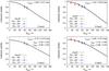 |
Fig. 2 Top: H-band (left) and K-band (right) visibilities of S CrA N together with ring-fit models (described in Sect. 3.1) consisting of a circular symmetric ring (ring width = 20% of inner ring radius rring,in) and an unresolved stellar source. Bottom: models consisting of the same star+ring model as above, plus a fully resolved halo component. |
AMBER observations.
3. Modeling
3.1. Geometric models
To measure the characteristic size of the circumstellar environment in the H- and K-bands, we fitted geometric models to the visibilities. Figure 2 shows the observed visibilities and the fitted models, which consist of a ring (the ring width being 20% of the inner radius; Eisner et al. 2003; Monnier et al. 2005), a stellar point source, and an extended fully resolved halo (in only the lower two panels). This extended halo is assumed to represent the stellar light scattered off a large-scale circumstellar structure (Akeson et al. 2005b). The motivation for a ring fit is that the model intensity distribution is expected to have a dominant PUIR brightness (Natta et al. 2001; Dullemond et al. 2001). Ring-fit radii are often used in the literature to characterize the disk size of YSO and to discuss their location in the size-luminosity relation (e.g. Monnier & Millan-Gabet 2002; Dullemond & Monnier 2010).
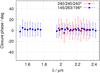 |
Fig. 3 Closure phases measured with AMBER in the H and K bands. |
The flux contribution fstar + fhalo from the star (fstar) plus a halo of scattered starlight (fhalo) was derived from the SED fit in Fig. 4 and amounts to 0.22 of the total flux (i.e. fstar + fhalo + fdisk) in the K band (2.2 μm) and 0.40 in the H band (1.6 μm). The total visibility V can be described by  (1)where Vstar = 1 and Vhalo = 0.
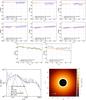 |
Fig. 4 Temperature-gradient model C of S CrA N – two top rows: NIR visibility. The model that fits visibility and SED simultaneously (model C in Table 4) is indicated with the solid red lines. The six figures show the modeling of the data sets I (top) and II (bottom), described in Table 2. Third row: MIDI visibility. The two figures show the comparison between our model (red line) and MIR data adopted from Schegerer et al. (2009). Bottom left: spectral energy distribution. To model the SED of S CrA N, we collected values from the literature and binned them (black dots are the dereddened SED points, see Appendix A). The green line represents the MIDI spectrum of Schegerer et al. (2009). The SED of model C is indicated with the blue line. It consists of the stellar contribution (Kurucz model, black dashed line) plus the contribution of two additional ring-like structures (black solid and dash-dotted line). Bottom right: intensity distribution of the temperature-gradient disk of model C. The dashed white ring indicates the expected dust sublimation radius of 0.05 AU predicted by the size-luminosity-relation (see Sect. 4). |
In fitting the data, we averaged the visibility data in each of the two bands. The H band visibilities were averaged over the wavelength range of ≈1.55–1.75 μm and the K band visibilities over ≈ 1.95–2.40 μm.
For the inner fit radius rring,in, we obtained 0.73 ± 0.03 mas in the H band and 0.85 ± 0.07 mas in the K band. The linear radii in AU for a distance of 130 pc (see Table 1) are listed in Table 3.
Ring-fit parameters in the H and K bands.
To test whether an elongation of the object can be measured, we also fitted an elliptic ring model. However, we were unable to detect any significant elongation. Because of the errors in the data, we can only derive a rough estimate of the elongation of < 30%. Therefore, we assume in the following modeling that the disk is oriented approximately face-on.
Overview of the parameter space scanned for the temperature-gradient models and parameters (with errors) of the best-fit models for one temperature-gradient disk (A, B) and two temperature-gradient disk components (C, D, E).
3.2. Temperature-gradient disk model
In this section, we present temperature-gradient models to help us interpret our observations. Each temperature-gradient model is the sum of many rings that emit blackbody radiation with temperatures T(r). For the temperature distribution, a power law is assumed (Hillenbrand et al. 1992), of T(r) = T0(r/r0) − q. Here, T0 is the effective temperature at a reference radius r0. The parameter q depends on the disk morphology and is predicted to be 0.50 for flared irradiated disks and either 0.75 for standard viscous disks or flat irradiated disks (Chiang & Goldreich 1997). Wavelength-dependent visibilities and fluxes of these model disks depend on the disk inclination, the inner radius rin, the outer radius rout, the temperature Tin at rin, and the temperature power-law index q. As explained in Sect. 3.1, we assumed that the disk is viewed face-on.
To determine the best temperature-gradient model, we calculated the model disks (one- and two-component structures) for all combinations of the parameters with scan ranges described in Table 4 (≈400 000 models). The total  is a sum over the
  of all visibility points for all six AMBER baselines and two MIDI baselines (see Schegerer et al. 2009), and the SED. We computed all combinations by running the model for six to ten steps per parameter and then chose the areas with the smallest value of to obtain a finer mesh. We took into account only wavelengths with λ < 20 μm. The errors in the best-fit model parameters are 1-σ errors.
The model assumes a stellar point source with the parameters T∗ = 4800 K, L∗ = 2.3 L⊙, distance = 130 pc, and Av = 2.8 (see references for the stellar parameters in Table 1). The model parameters of all derived models (disk plus star, disk plus star plus halo, as well as several two-component disks) are listed in Table 4.
3.2.1. One-component temperature-gradient disk models
The simplest temperature-gradient model A (see Table 4) consists of only one single disk component plus the star. It cannot reproduce the SED as well as the MIR and NIR visibilities simultaneously ( 17).
17).
For the star-disk-halo model B, we added a fully resolved halo (V = 0) to the star-disk model A. This halo intensity distribution is assumed to represent the stellar light scattered off the large-scale circumstellar material and to have approximately the same SED as the star itself (cf. Akeson et al. 2005b). Nevertheless, the improvement achieved was very small since the became only 11.5 (see Table 4). We also computed 20 star-disk-halo models with resolved halos of different widths in the range from 0.05 AU to 100 AU, but the did not significantly improve since it remained larger than ≈ 11.5 in all cases. As in the case of model A without a halo, it was only possible to fit either the SED and the AMBER measurements or the SED and the MIDI measurements. This suggests that a more complicated disk structure should be considered. Therefore, we introduced a second disk component in the following, but – as we preferred to adopt a two-disk modeling with a minimum number of free parameters – we omitted the weak halo.
3.2.2. Two-component temperature-gradient disk models
Model C is the result of our attempt to find a two-disk component model with the least number of parameters (Table 4). We therefore introduced constraints on the inner and outer radii and temperatures of disks 1 and 2, of Tout,1 = Tin,2 and rout,1 = rin,2. We obtained  (the power-law index q1 is determined from the temperature slope between rin,1 and rout,1 and is therefore no longer a free parameter).
We also tested models with more parameters: in model D, rout,1 = rin,2 is the only constraint and  . For model E, there are no constraints, but we still get a similar (3.0). Table 4 shows that only models C to E have a from 3.0 to 3.2 and among those, model C has the advantage that it has the smallest number of parameters.
Figure 4 shows the intensity distribution of model C, together with all S CrA N observations. An extended ring is located between 0.14 AU and 26 AU, whereas the inner ring extends radially from 0.11 AU to 0.14 AU and has a temperature of 1690 K at the inner ring edge (see parameters in Table 4).
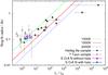 |
Fig. 5 Location of S CrA N in the size-luminosity diagram: K-band ring-fit radii derived with a geometric ring-star model (pink square, ≈ 0.13 AU) and a ring-star-halo model (blue square, ≈ 0.11 AU); see Tables 3 and 1 for the stellar parameters used. The lines indicate the predicted theoretical dependence of the K-band radius on the luminosity (Monnier & Millan-Gabet 2002). Predictions of models including backwarming are discussed in Sect. 4. The filled black squares are a sample of Herbig Ae stars (Monnier et al. 2005). The open black squares represent a sample of TTS (Pinte et al. 2008). |
4. Discussion
For comparison with other pre-main sequence stars, we plot the geometric K-band ring-fit radii, where rring,in ≈ 0.13 AU for the geometric model without a halo and ≈ 0.11 AU for the model with a halo; Sect. 3.1, of S CrA N in the size-luminosity diagram that shows the K-band ring-fit radius as a function of the stellar luminosity L ∗ (Monnier & Millan-Gabet 2002, Fig. 5). The figure shows a sample of Herbig Ae stars (filled squares, Monnier et al. 2005), for which this correlation has been originally found. Additionally, we plot a sample of TTS (open squares, Pinte et al. 2008).
Figure 5 shows that our measurements of the K-band ring-fit radius of S CrA N of ≈ 0.11 − 0.13 AU, radii derived with the geometric ring-star and ring-star-halo models, is approximately 2.4 times larger than the dust sublimation radius of ≈ 0.05 AU predicted for the silicate dust sublimation temperature of 1500 K and gray dust opacities (Monnier & Millan-Gabet 2002). However, several effects can influence the inner model radius, such as the chemistry and grain size of the dust (e.g. Monnier & Millan-Gabet 2002) or magnetospherical disk truncation (Eisner et al. 2007). Schegerer et al. (2009) modeled their mid-infrared MIDI data and the SED of S CrA N using the Monte Carlo code MC3D (Wolf et al. 1999; Schegerer et al. 2008). They found that an assumed sublimation radius of 0.05 AU agrees with their observations.
Furthermore, we compared our ring-fit radii of ≈ 0.11 − 0.13 AU derived from the geometric star-disk and star-disk-halo models and the inner disk radii of our temperature-gradient models (0.11–0.14 AU) with the predictions of a model that accounts for both backwarming and accretion luminosity (Millan-Gabet et al. 2007; Dullemond & Monnier 2010). This model suggests an inner disk radius of 0.12 AU for a stellar luminosity of 2.3 L⊙ and an accretion luminosity of 0.6 L⊙ (derived from Prato et al. 2003; Muzerolle et al. 1998), which agrees with our measured inner radius of ≈ 0.11–0.13 AU.
5. Conclusions
We have observed the T Tauri star S CrA N with AMBER in the H and K bands. We have fitted the geometric star-disk and star-disk-halo models to our visibility data and derived a radius rring,in of approximately 0.11 − 0.13 AU in the K band (0.095–0.12 AU in the H band). We compared the position of S CrA N in the size-luminosity diagram with the position of other YSO, and found that it is above the line expected for a dust sublimation temperature of 1500 K and gray dust, but within the region of other TTS. The radius predicted by this size-luminosity relation is ≈ 0.05 AU, whereas the derived ring-fit radius is ≈ 0.11 − 0.13 AU (Table 3). However, models including backwarming (Millan-Gabet et al. 2007; Dullemond & Monnier 2010) suggest a larger inner disk radius of ≈ 0.12 AU, which agrees with our derived ring-fit radiii of ≈ 0.11 − 0.13 AU.
We tested several temperature-gradient models (one- and two-component disk models, with or without halo). We found that the near- and mid-IR visibilities, as well as the SED, can approximately be reproduced by a temperature-gradient model consisting of a two-component ring-shaped disk and an unresolved star. The favored temperature-gradient model C (see Table 4) has a temperature of ≈ 1700 K at the inner disk radius of 0.11 AU. The temperature power-law index q1 of the inner narrow temperature-gradient disk is approximately 0.2, and the index q2 of the extended outer disk is approximately 0.5, which suggests a flared irradiated disk structure (Chiang & Goldreich 1997). However, q1 is not well-constrained because of the narrow width of the inner component of only ≈ 0.03 AU. The inner temperature-gradient disk radius of 0.11 AU is similar to the four geometric ring-fit radii of approximately 0.10 AU to 0.13 AU and to the prediction of models including backwarming (0.12 AU). Unfortunately, we cannot place any constraints on the gas within the inner disk radius of ≈ 0.11 AU since the disk is only partially resolved (all NIR visibilities are > 0.77) and the visibility errors are large. Interestingly, the inner disk components of all three best-fit temperature-gradient models consist of a very narrow, hot ring (Tin,1 ≈ 1500–1700 K; ring width only ≈ 0.03–0.04 AU) surrounded by a colder (<600 K) disk component with an extension of several AU. This size and temperature structure is similar to the structure of more sophisticated radiative transfer models including a hot PUIR (e.g., Natta et al. 2001; Dullemond et al. 2001). This suggests that the derived narrow, inner disk component in the temperature-gradient models is caused by a hot, perhaps PUIR, in S CrA N. This rim may explain the steep temperature jump from 1500 K to 600 K.
Acknowledgments
J. Vural was supported for this research through a stipend from the International Max Planck Research School (IMPRS) for Astronomy and Astrophysics at the Universities of Bonn and Cologne.
References
- Akeson, R. L., Boden, A. F., Monnier, J. D., et al. 2005a, ApJ, 635, 1173 [NASA ADS] [CrossRef] [Google Scholar]
- Akeson, R. L., Walker, C. H., Wood, K., et al. 2005b, ApJ, 622, 440 [NASA ADS] [CrossRef] [Google Scholar]
- Bonsack, W. K. 1961, ApJ, 133, 340 [NASA ADS] [CrossRef] [Google Scholar]
- Carmona, A., van den Ancker, M. E., & Henning, T. 2007, A&A, 464, 687 [NASA ADS] [CrossRef] [EDP Sciences] [Google Scholar]
- Chiang, E. I., & Goldreich, P. 1997, ApJ, 490, 368 [NASA ADS] [CrossRef] [Google Scholar]
- Cieza, L. A., Kessler-Silacci, J. E., Jaffe, D. T., Harvey, P. M., & Evans, II, N. J. 2005, ApJ, 635, 422 [NASA ADS] [CrossRef] [Google Scholar]
- Dullemond, C. P., & Monnier, J. D. 2010, ARA&A, 48, 205 [NASA ADS] [CrossRef] [Google Scholar]
- Dullemond, C. P., Dominik, C., & Natta, A. 2001, ApJ, 560, 957 [NASA ADS] [CrossRef] [Google Scholar]
- Eisner, J. A., Lane, B. F., Akeson, R. L., Hillenbrand, L. A., & Sargent, A. I. 2003, ApJ, 588, 360 [NASA ADS] [CrossRef] [Google Scholar]
- Eisner, J. A., Hillenbrand, L. A., White, R. J., et al. 2007, ApJ, 669, 1072 [NASA ADS] [CrossRef] [Google Scholar]
- Ghez, A. M., McCarthy, D. W., Patience, J. L., & Beck, T. L. 1997, ApJ, 481, 378 [NASA ADS] [CrossRef] [Google Scholar]
- Graham, J. A. 1992, PASP, 104, 479 [NASA ADS] [CrossRef] [Google Scholar]
- Herbig, G. H., & Bell, K. R. 1988, Third Catalog of Emission-Line Stars of the Orion Population, eds. G. H. Herbig, & K. R. Bell, 3 [Google Scholar]
- Hillenbrand, L. A., Strom, S. E., Vrba, F. J., & Keene, J. 1992, ApJ, 397, 613 [NASA ADS] [CrossRef] [Google Scholar]
- Kharchenko, N. V., & Roeser, S. 2009, VizieR Online Data Catalog, I/280 [Google Scholar]
- Kreplin, A., Kraus, S., Hofmann, K.-H., et al. 2012, A&A, 537, A103 [NASA ADS] [CrossRef] [EDP Sciences] [Google Scholar]
- McCabe, C., Ghez, A. M., Prato, L., et al. 2006, ApJ, 636, 932 [NASA ADS] [CrossRef] [Google Scholar]
- Millan-Gabet, R., Malbet, F., Akeson, R., et al. 2007, Protostars and Planets V, 539 [Google Scholar]
- Monnier, J. D., & Millan-Gabet, R. 2002, ApJ, 579, 694 [NASA ADS] [CrossRef] [Google Scholar]
- Monnier, J. D., Millan-Gabet, R., Billmeier, R., et al. 2005, ApJ, 624, 832 [NASA ADS] [CrossRef] [Google Scholar]
- Muzerolle, J., Hartmann, L., & Calvet, N. 1998, AJ, 116, 2965 [NASA ADS] [CrossRef] [Google Scholar]
- Muzerolle, J., Calvet, N., Hartmann, L., & D’Alessio, P. 2003, ApJ, 597, L149 [NASA ADS] [CrossRef] [Google Scholar]
- Natta, A., Prusti, T., Neri, R., et al. 2001, A&A, 371, 186 [NASA ADS] [CrossRef] [EDP Sciences] [Google Scholar]
- Neuhäuser, R., & Forbrich, J. 2008, The Corona Australis Star Forming Region, ed. B. Reipurth, 735 [Google Scholar]
- Ortiz, J. L., Sugerman, B. E. K., de La Cueva, I., et al. 2010, A&A, 519, A7 [NASA ADS] [CrossRef] [EDP Sciences] [Google Scholar]
- Patten, B. M. 1998, in Cool Stars, Stellar Systems, and the Sun, eds. R. A. Donahue, & J. A. Bookbinder, ASP Conf. Ser., 154, 1755 [Google Scholar]
- Petrov, R. G., Malbet, F., Weigelt, G., et al. 2007, A&A, 464, 1 [NASA ADS] [CrossRef] [EDP Sciences] [Google Scholar]
- Pinte, C., Ménard, F., Berger, J. P., Benisty, M., & Malbet, F. 2008, ApJ, 673, L63 [NASA ADS] [CrossRef] [Google Scholar]
- Prato, L., Greene, T. P., & Simon, M. 2003, ApJ, 584, 853 [NASA ADS] [CrossRef] [Google Scholar]
- Reipurth, B., & Graham, J. A. 1988, A&A, 202, 219 [NASA ADS] [Google Scholar]
- Reipurth, B., & Zinnecker, H. 1993, A&A, 278, 81 [NASA ADS] [Google Scholar]
- Richichi, A., Percheron, I., & Khristoforova, M. 2005, A&A, 431, 773 [NASA ADS] [CrossRef] [EDP Sciences] [Google Scholar]
- Schegerer, A. A., Wolf, S., Ratzka, T., & Leinert, C. 2008, A&A, 478, 779 [NASA ADS] [CrossRef] [EDP Sciences] [Google Scholar]
- Schegerer, A. A., Wolf, S., Hummel, C. A., Quanz, S. P., & Richichi, A. 2009, A&A, 502, 367 [NASA ADS] [CrossRef] [EDP Sciences] [Google Scholar]
- Tatulli, E., Millour, F., Chelli, A., et al. 2007, A&A, 464, 29 [NASA ADS] [CrossRef] [EDP Sciences] [Google Scholar]
- Walter, F. M., & Miner, J. 2005, in 13th Cambridge Workshop on Cool Stars, Stellar Systems and the Sun, eds. F. Favata, G. A. J. Hussain, & B. Battrick, ESA SP, 560, 1021 [Google Scholar]
- Wang, H., Mundt, R., Henning, T., & Apai, D. 2004, ApJ, 617, 1191 [NASA ADS] [CrossRef] [Google Scholar]
- Wolf, S., Henning, T., & Stecklum, B. 1999, A&A, 349, 839 [NASA ADS] [Google Scholar]
Appendix A: SED references
To simplify the fitting process, we did not use the pile of original data (Table A.1), but instead binned them to form a smaller number of data points. Figure A.1 shows both the original data (blue crosses) and the binned data (red dots). The measurements were not recorded contemporaneously (see Table A.1) and therefore variability is one of the error sources. Other SED error sources are the different aperture sizes and the small number of observations in the visible and NIR.
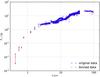 |
Fig. A.1 SED of S CrA N – original data according to the sources in Table A.1 (blue crosses) and the binned data (red dots). |
Measurements from the literature that were used to produce the binned SED of S CrA N.
All Tables
Overview of the parameter space scanned for the temperature-gradient models and parameters (with errors) of the best-fit models for one temperature-gradient disk (A, B) and two temperature-gradient disk components (C, D, E).
Measurements from the literature that were used to produce the binned SED of S CrA N.
All Figures
|
Fig. 1 The uv coverage of the AMBER (red and green dots) and MIDI (blue and pink squares) observations used for modeling. |
| In the text | |
|
Fig. 2 Top: H-band (left) and K-band (right) visibilities of S CrA N together with ring-fit models (described in Sect. 3.1) consisting of a circular symmetric ring (ring width = 20% of inner ring radius rring,in) and an unresolved stellar source. Bottom: models consisting of the same star+ring model as above, plus a fully resolved halo component. |
| In the text | |
|
Fig. 3 Closure phases measured with AMBER in the H and K bands. |
| In the text | |
|
Fig. 4 Temperature-gradient model C of S CrA N – two top rows: NIR visibility. The model that fits visibility and SED simultaneously (model C in Table 4) is indicated with the solid red lines. The six figures show the modeling of the data sets I (top) and II (bottom), described in Table 2. Third row: MIDI visibility. The two figures show the comparison between our model (red line) and MIR data adopted from Schegerer et al. (2009). Bottom left: spectral energy distribution. To model the SED of S CrA N, we collected values from the literature and binned them (black dots are the dereddened SED points, see Appendix A). The green line represents the MIDI spectrum of Schegerer et al. (2009). The SED of model C is indicated with the blue line. It consists of the stellar contribution (Kurucz model, black dashed line) plus the contribution of two additional ring-like structures (black solid and dash-dotted line). Bottom right: intensity distribution of the temperature-gradient disk of model C. The dashed white ring indicates the expected dust sublimation radius of 0.05 AU predicted by the size-luminosity-relation (see Sect. 4). |
| In the text | |
|
Fig. 5 Location of S CrA N in the size-luminosity diagram: K-band ring-fit radii derived with a geometric ring-star model (pink square, ≈ 0.13 AU) and a ring-star-halo model (blue square, ≈ 0.11 AU); see Tables 3 and 1 for the stellar parameters used. The lines indicate the predicted theoretical dependence of the K-band radius on the luminosity (Monnier & Millan-Gabet 2002). Predictions of models including backwarming are discussed in Sect. 4. The filled black squares are a sample of Herbig Ae stars (Monnier et al. 2005). The open black squares represent a sample of TTS (Pinte et al. 2008). |
| In the text | |
|
Fig. A.1 SED of S CrA N – original data according to the sources in Table A.1 (blue crosses) and the binned data (red dots). |
| In the text | |
Current usage metrics show cumulative count of Article Views (full-text article views including HTML views, PDF and ePub downloads, according to the available data) and Abstracts Views on Vision4Press platform.
Data correspond to usage on the plateform after 2015. The current usage metrics is available 48-96 hours after online publication and is updated daily on week days.
Initial download of the metrics may take a while.