| Issue |
A&A
Volume 543, July 2012
|
|
|---|---|---|
| Article Number | A51 | |
| Number of page(s) | 7 | |
| Section | Stellar structure and evolution | |
| DOI | https://doi.org/10.1051/0004-6361/201218845 | |
| Published online | 25 June 2012 | |
Molecular hydrogen jets and outflows in the Serpens South filamentary cloud⋆
1 Centro de Astrofísica da Universidade do Porto, Rua das Estrelas, 4150-762 Porto, Portugal
e-mail: This email address is being protected from spambots. You need JavaScript enabled to view it.
2 Observatorio Astronómico Nacional (IGN), Calle Alfonso XII 3, 28014 Madrid, Spain
Received: 19 January 2012
Accepted: 19 April 2012
Abstract
Aims. We map the jets and outflows from the Serpens South star-forming region and find an empirical relationship between the magnetic field and outflow orientation.
Methods. We performed near-infrared H2v = 1−0 S(1) 2.122 μm – line imaging of the ~30′ – long filamentary shaped Serpens South star-forming region, and used Ks broadband imaging of the same region for the continuum subraction. Candidate driving sources of the mapped jets/outflows are identified from the list of known protostars and young stars in this region, which was derived from studies using Spitzer and Herschel telescope observations.
Results. We identify 14 molecular hydrogen emission-line objects (MHOs) in our continuum-subtracted images. They are found to constitute ten individual flows. Among these, nine flows are located in the lower-half(southern) part of the Serpens South filament, and one flow is located at the northern tip of the filament. Four flows are driven by well-identified Class 0 protostars, while the remaining six flows are driven by candidate protostars mostly in the Class I stage, based on Spitzer and Herschel observations. The orientation of the outflows is systematically perpendicular to the direction of the near-infrared polarization vector published in the literature. No significant correlation was observed between the orientation of the flows and the axis of the filamentary cloud.
Key words: stars: formation / open clusters and associations: individual: Serpens South / infrared: stars / ISM: clouds / ISM: jets and outflows
Figure 5 is available in electronic form at http://www.aanda.org
© ESO, 2012
1. Introduction
Star formation is thought to occur in molecular clouds, which are largely known to have a filamentary structure caused primarily by the turbulence that acts within them (Nakamura et al. 2011). Our understanding of the details of star formation is largely based on observational studies of clean templates of nearby filamentary molecular clouds. A recently discovered filamentary cloud and its associated protocluster (Gutermuth et al. 2008) in Serpens South can be used as one such template.
The Serpens South protocluster is located at the center of a well-defined filamentary cloud that appears as a dark patch in the Spitzer 8 μm image with an approximate extent of 30′ in length, and is thought to be part of the larger Serpens-Aquila rift molecular cloud complex (Bontemps et al. 2010; Gutermuth et al. 2008; André et al. 2010). The short distance to this region of ~260 pc (Gutermuth et al. 2008; Bontemps et al. 2010) places it among one of the nearest star-forming regions, making it an interesting target for studies of star formation.
A swath of new infrared and submillimeter observations has been used to study various aspects of this star-forming cloud. Gutermuth et al. (2008) used Spitzer-IRAC observations to uncover the embedded young star population. Bontemps et al. (2010) presented submillimeter observations performed with the Herschel Space Telescope and identified several Class 0 protostars and candidate protostars in, and around, the filament. Sugitani et al. (2011) mapped the magnetic field associated with this filamentary cloud using near-infrared polarimetric observations. Molecular outflows in this region were traced by Nakamura et al. (2011) using CO(J = 3 − 2) observations. Together, these observations have permitted a rich characterization of the Serpens South star-forming region to be made.
The motivation for the study presented in this paper primarily arose from the availability of magnetic field measurements of the entire filament. It is well-known based on star-formation theories, that the bipolar outflows in young stars are ejected in the direction of the polar axis, along which the magnetic field is also aligned (Tamura et al. 1989). In particular, there is some indication that the outflow activity is orthogonally aligned with the axis of a filamentary cloud (Anathpindika & Whitworth 2008), because the formation of prestellar cores is fuelled by inflows along the filament (Banarjee et al. 2006). It is possible that an ordered magnetic field on the global scale of the filament may be related to a stronger coherence of the orientation of the outflows with the cloud axis. For example, in the DR21/W75 region, a statistically significant coherence was found in the direction of the flows (Davis et al. 2007; Kumar et al. 2007). The magnetic field measurements of this region presented by Kirby (2009) agreed quite well with previous results in terms of the alignment between the magnetic field and the cloud axis. However, similar outflow studies in the Orion A cloud did not identify any significant correlation of the orientation of the outflows with the filamentary axis (Davis et al. 2009). This lack of consistency between the results obtained for these two different regions does not allow us to establish whether there is a relation between the orientation of these two components of star formation.
Although many outflow components were found for the Serpens South filament by Nakamura et al. (2011), the lower spatial resolution of the radio observations, and the high density of young stars in the protocluster makes it difficult to identify and clearly relate the outflow activity to the protostars. Here, we present deep H2 narrow-band imaging study of the entire Serpens South filament to a) identify the individual components of the flows by building upon the results of Nakamura et al. (2011); b) associate the flows with the most likely driving source; and c) compare the orientations of the flows with both that of the global magnetic field measured by Sugitani et al. (2011) and the axis of the filamentary cloud.
2. Observations
Near-infrared observations were carried out on the nights of 14−17 July 2011 using the 3.5 m telescope at the German-Hispanic Astronomical Center at Calar Alto (CAHA). Two pointings were targeted in order to cover the full filament (Gutermuth et al. 2008). We used a near-infrared wide-field camera, Omega2000, with a 15.3′ field of view and a plate scale of 0.45′′ per pixel.
Observations in the H2v = 1−0 S(1) 2.122 μm narrow-band filter were made by applying a nine-point jitter sequence and were repeated eight times for each pointing. An exposure time of 60 s per jitter was fixed, resulting in an integration time of ~72 min. To facilitate continuum subtraction, observations in the Ks broadband filter were obtained using a twenty-point jitter pattern, rerun one additional time at each pointing, with an exposure time of 5 s, so that the final integration time was ~4 min.
Each set of jittered images were median-combined to obtain a sky-frame that was then subtracted from each individual image. The alignment of each image was performed using CCDPACK routines in the Starlink1 suite of software. The final mosaics were achieved using KAPPA and CCDPACK routines in the Starlink.
The Ks broadband images were matched in terms of their point spread function and their relative fluxes were scaled to help us to perform the continuum subtraction of the H2 images.
 |
Fig. 1 Continuum-subtracted H2 image of the southern part of the observed region, displayed with logarithmic scales. The sources are marked according to the following: diamonds represent Class 0 stars from Bontemps et al. (2010), circles are Class I from Bontemps et al. (2010), and the square is a candidate Class 0 observed only in Spitzer 24 μm , the labels P2, P3, P4, P5, Y1, Y2, Y3, Y4, and Y5 are the names we used to refer to each source throughtout our work. For more on the outflows and driving sources, see Table 1. As dashed lines, we also show the polarization vectors (Sugitani et al. 2011). |
3. Results
The continuum-subtracted H2 images from our observations cover almost the entire Serpens South filament, which is roughly 30′ in length. However, only two sub-regions display all the detected H2 emission. Figure 1 shows the southern part of the filament where most of the H2 emission is detected. The northern part of the filament is less active, the region with detected emission is shown in Fig. 2.
In these figures, the detected H2 features are labeled by their molecular hydrogen emission-line object (MHO) names following the catalog system described by Davis et al. (2010). When MHOs are associated with clear bipolar outflows, we use the same catalog number for both lobes, but we add the suffix of either “b” or “r” depending on whether it is, respectively, the blue-shifted or red-shifted lobe.
In naming the MHO features, we first identified all possible bipolar flows and their driving sources as explained below. We started by identifying bowshock-like features. We then extended a line tracing the middle of the bowshock until we reached a possible outflow counterpart. When this counterpart exists, the driving source of the MHO should be along the traced line. The driving sources were assumed to be either previously identified Class 0 objects (Bontemps et al. 2010) or Class I objects (Gutermuth et al. 2008). In almost all cases, a suitable driving source was found. When a bipolar outflow was identified, the MHO lobe further away in the plane of the sky from the source was assumed to be the blue-shifted lobe, while the one closer to the source was assumed to be the red-shifted lobe.
After the well-defined bipolar flows were identified, the remaining MHO features were associated with the most likely driving source, with the aid of Spitzer data and the CO maps published by Nakamura et al. (2011). In Fig. 1, all identified flows are indicated by solid lines. Diamond symbols represent Class 0 protostars and open circles Class I young stars. Figure 5 is a color composite made in which the Spitzer MIPS 24 μm image is indicated in red, the IRAC 8.0 μm image in green, and the H2 image in blue. This figure covers exactly the same region displayed in Fig. 1 and reveals the dark filament. The CO flows discovered by Nakamura et al. (2011) are also overlaid on this figure, which demonstrates how well the identified H2 flows correspond to the CO emission.
A total of ten flows were identified in the entire Serpens South filament (Figs. 1 and 2), among which five were clearly identified as bipolar. In the remaining MHOs, we detected H2 emission only from one of the lobes. Two well-defined jet-like features and one bipolar nebula delineated by a dark lane (indicating a disk) are also identified. These interesting features are shown in Fig. 3.
In the following, we first discuss in detail each flow explaining their morphology and the nature of the identified driving sources. Table 1 lists the coordinates and morphology of the MHOs. In Table 2, we list the driving sources, their evolutionary class, and their visibility in various infrared and millimeter bands.
List of MHOs and their sources.
3.1. Cataloged MHOs
MHO 2214b and MHO2214r: MHO2214 is a well-defined bipolar outflow (Fig. 2), with collimated components. Its blueshifted component was previously discovered by Connelley et al. (2007), but our observations were the first to reveal its redshifted counterpart, thus enabling us to discover its bipolar nature. The central knot of the blue-shifted component is a distinct bowshock. The source P1, which is identified as the driving source, was classified as a protostar by Bontemps et al. (2010), and is located equidistantly from both MHO features.
MHO 3247: this MHO feature is represented in Fig. 1 by a dashed arrow indicating its probable direction. It is a jet-like feature originating from the source P2, which was classified as a Class 0 protostar by Bontemps et al. (2010) and located in the midst of the protocluster discovered by Gutermuth et al. (2008). No discernable MHO counterpart was found for this feature. We note that this region is the central part of the filament, which is associated with a dense cluster of young stars and intense, multiple outflow activity (Nakamura et al. 2011) causing much confusion in the counterpart identification.
MHO 3248: this is a bright MHO feature with a relatively wide opening angle. When compared with the CO maps of Nakamura et al. (2011), it shows clear indications of extending to the south by ~317 arcsec, touching the bowshock feature identified as MHO3251b. The most likely driving source of this MHO feature is the Class 0 object marked as P3 in Fig. 1, and located in the middle of the Serpens South protocluster. This MHO feature appears to be associated with the blue lobes MHO3249b and MHO3251b, the outflows of which it has likely had a previous physical interaction.
 |
Fig. 2 Continuum-subtracted H2 image of the northern part of the observed region, displayed on logarithmic scales. This bipolar outflow is well-aligned with the Class 0 protostar P1 (Bontemps et al. 2010). |
MHO 3249b, MHO3249r: these MHO features are identified to delineate a bipolar-flow driven by the Class I young star P4 (Bontemps et al. 2010), which appears as an infrared point source and is associated with significant millimeter continuum-emission. The southern blue lobe ends in a clear, sharply defined bowshock. The red-shifted component has a single, poorly defined knot but that it is well-aligned with the source and the blue-shifted lobe allows us to determine that they are part of the same bipolar flow. MHO3249b shows indications of crossing and/or being physically in contact with the outflow lobe associated with MHO3248. Nevertheless, the well-defined bowshock associated with this lobe unambiguously identifies the outflow lobe and the driving source.
MHO 3250: MHO3250 is composed of two visible H2 knots and delineates one of the lobes of an outflow driven by the Class I young star marked as Y1. There is some indication that this poorly defined MHO crosses paths with another nearby flow associated with MHO3251r.
MHO 3251b, MHO3251r: these MHO features are associated with a well-identified bipolar outflow, originating in the Class I young star Y2 (Bontemps et al. 2010). The red and blue lobes are nearly equidistant from the source (see Fig. 1), suggesting that this flow is in the plane of the sky. This idea is supported by the detection of a clear, bipolar-shaped nebula visible in the Ks band images. The bipolar nebula is divided by a dark strip showing a clear sign of an edge-on disk in the source, a zoomed image of which is displayed in Fig. 3a. The MHO features are aligned perpendicularly to the disk feature, the blue lobe MHO3251b terminating in a well-defined bowshock and MHO3251r being composed of two knots. The presence of another MHO, MHO3250, near the red-shifted component is a source of some confusion but not so as to significantly change our conclusions.
MHO 3252b, MHO3252r: these MHO features are away to the south of the confusing central protocluster. MHO3252b consists of a clear H2 jet originating from the Class I young star marked as Y3 (Bontemps et al. 2010). The YSO is visible even in the near-infrared Ks band and is also associated with a clear millimeter core identified from Herschel observations. The blue-shifted lobe driven by this source terminates in a distinct arc-like H2 feature, while the red-shifted lobe is traced by a group of H2 knots. This flow is bright enough to be prominently visible even in the color composite image (see Fig. 5).
List of driving sources.
 |
Fig. 3 From left to right, the images are centered on the bipolar nebula of Y2 visible in the Ks broadband filter, the outflow jet from Y3 in a continuum-subtracted image, and the jet from P2, which is also in a continuum-subtracted image. |
MHO 3253: MHO3253 could be classified as a bipolar outflow but since part of the outflow crosses MHO3254 we only address the northern lobe, a clear arc-like structure originating in the nearby Class I source, Y4 (Bontemps et al. 2010).
MHO 3254: this feature is probably associated with a flow driven by a Class I YSO, marked as Y5 in Fig. 1. The eastern part of this ouflow shows a single knot in the direction of the source that overlaps with the possible bipolar flow originating from MHO3253, causing some confusion.
MHO 3255: this H2 feature has the morphology of a wiggly bowshock. At the outset, it is likely the tip of a very long flow originating from the Class 0 source P3, that is situated at the center of the protocluster. A careful analysis of Spitzer MIPS-24 μm images, nevertheless, reveals a faint source marked P5 in Fig. 1, located in the middle of this H2 emission. Furthermore, this faint MIPS source is also associated with weak millimeter continuum-emission that is identified by Herschel observations as a candidate protostar. We therefore, suggest that MHO3255 is a weak outflow with a very young age owing to the candidate protostar P5. The wiggly bow-shape of the H2 features may then be due to the motion of this source on the plane of the sky.
Finally, we examined the Spitzer 4.5 μm images analyzed by Gutermuth et al. (2008) to uncover any hidden census of outflows that might have escaped detection in our near-infrared data. The Spitzer-IRAC 4.5 μm band is known to encompass a bright H2 emission line, and, the extinction at this wavelength is roughly half as much as in the K band (Flaherty et al. 2007). Although almost all of our detected outflows are also present in those images, there is no visible indication of additional outflows in the studied area. The H2 data presented here indeed provide us with confidence that we detected pure emission-line features unlike the 4.5 μm data where judgement is based on comparisions with other bands and not on real continuum subtraction. Furthermore, our H2 data have a higher spatial resolution than Spitzer which permits us to clearly distinguish the morphological details. That we do not detect additional features from Spitzer data indicates that the outflow sample traced by our data is quite complete and the extinction in this cloud is similar to other nearby regions of star formation where H2 narrow-band images effectively serve as jet/outflow tracers.
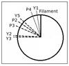 |
Fig. 4 Positional angles(PA) of the sources polarization relative to the PA of the filament (0 degrees). Solid and dashed lines correspond to PA < 45° and PA > 45°, respectively. |
4. Discussion
In the studied region, we have detected a total of ten outflows, five of which are clearly bipolar, and in the remaining five MHOs only a single lobe. We then studied the collimation factors of each MHO, which is defined as the ratio of the length to the width of each outflow. At least two of the observed MHOs have high collimation factors, particularly MHO3249r and MHO3254, which have collimation factors of 11.2 and 15.6 respectively. These examples of extreme collimation can be directly linked to the young nature of these sources and may be an indication of high velocity components (Bachiller 1996). On the other hand, we also observe some outflows that have low collimation factors (of between 5 and 5), MHO3253, MHO3252r, and MHO2214b with factors of 2.5, 4.2, and 4.6, respectively. These low collimation factors point towards the origin of these outflows being in ambient gas picked up by stellar winds (Bachiller 1996).
We also performed a rough comparison between the orientation of the MHOs and the axis of the cloud filament. Outflows were considered to be parallel to the filament if their orientation angle with respect to the axis of the filament is less than 45 and perpendicular when the angle was greater than 45. This comparison showed that ~71% of the flows are perpendicular and ~29% are parallel to the filament. In Fig. 4, we plotted the positional angles (PA) of the known polarization vectors relative to the PA of the filament or subfilament where each source is located, in order to observe the distribution of the parallel and perpendicular vectors. Although these fractions are similar to the values obtained by Anathpindika & Whitworth (2008) (~72% perpendicular and ~28% parallel), we stress that our sample is not large enough to be statistically significant. Although we cannot discern a coherent pattern in the orientation of the outflows owing to the low quality statistics of our data, our analysis demonstrates that the fraction of flows perpendicular to the filament are clearly larger than those parallel to the filament.
Nevertheless, we found that there is a stronger correlation between the orientation of the outflows with respect to the local magnetic field. To obtain this result, we compared the direction of the MHO flows with that of the near-infrared polarization vectors of the driving sources (obtained from the data of Sugitani et al. 2011). We were able to find polarization vectors associated with seven identified driving sources, namely P2, P3, P4, Y1, Y2, Y3, and Y5. These vectors are shown as dashed lines in Fig. 1. In all of these cases, the outflows are generally found to be perpendicular to the polarization vectors. In particular, the polarization vector of source Y2 perfectly traces the disk of that young star (see Fig. 3), which is identified as a dark lane cutting across a bipolar reflection nebula, and is found to be perpendicular to MHO3251.
The polarization measurements of light from young stars are known to represent the disks and envelopes rather than the embedded proto-star. This is because the light originating in the young star is reprocessed in the dense envelopes surrounding them before reaching the observer. Therefore, the observed polarization vectors are usually found to be parallel to the disk axis, which is perpendicular to the axis of the stellar magnetic field (Tamura et al. 1989; Pereyra et al. 2009; Murakawa 2010). The level of polarization is found to be higher in younger sources and/or edge-on disks than in older sources (Greaves et al. 1997).
It is known that outflows follow the open magnetic lines of the source, which means that their origin should be near the magnetic poles of the source (Königl et al. 2011). Since the majority of the observed outflows are perpendicular to the known polarization vectors, we can conclude that the observed polarization vectors are perpendicular to the magnetic field of the driving sources. Given this close relation between the local magnetic field and the arrangement of MHOs, it is clear that the outflows are aligned with the local magnetic field. While the large-scale orientation of the polarization vectors runs roughly perpendicular to the axis of the filamentary cloud, local twists were found in the observations of Sugitani et al. (2011). The location of the driving sources along these twists may, therefore, indicate the position of star-forming cores. As accretion proceeds, the magnetic field appears to become distorted, hence we neither expect to nor actually observe any coherent alignment between the global magnetic field and the orientation of the MHOs (Pereyra et al. 2009). This is likely one of the reasons we do not find a high degree of coherence between the orientation of the flows with the filamentary axis. Other factors such as turbulence, the morphology of the filament on smaller scales, and the distribution of cores can also strongly influence the deviations of the local magnetic fields from the global field.
5. Summary and conclusions
We have discovered new MHO features in the filamentary molecular cloud “Serpens South” associated with a protocluster situated in the Aquila Rift. We have cataloged MHO features associated with ten outflows, five of which are clearly identified as bipolar outflows (Table 1). A comparison between our survey and previous images obtained with Spitzer demonstrated that there are no additional MHOs in the region. Two jet-like features, launched from the driving YSOs have been clearly identified. One edge-on disk in this region is also identified from this study (see the bipolar nebula in Fig. 3). Half of the detected
flows have been proposed to be driven by previously classified Class 0 objects and the remaining half by Class I type sources. The MHO features found here are clearly associated with the CO outflows presented by Nakamura et al. (2011). In particular, MHO3247, MHO3248, MHO3251, and MHO3252 appear to trace the CO maps extremely well because the blue or red shifted lobes can be clearly matched.
Two of the observed MHOs have high collimation factors, indicating that we are dealing with high velocity flows.
Our H2 imaging study has allowed us to identify and clarify the association between outflows and driving sources in the central protocluster. The high concentration of outflows from the protocluster located at the center of the filamentary cloud displayed some confusion that did not permit an unambiguous association of the outflows and their sources. Our results also indicate that the flows launched from the central protocluster might have interacted with each other physically since they are launched from a small region. MHO3248 and MHO3249b are two such signatures.
We have shown that the near-infrared polarization vectors mapped by Sugitani et al. (2011) are perpendicular to the outflows and therefore to the magnetic field of the sources. While the outflows are perpendicular to the local polarization vectors, no specific coherence is found with the global pattern. Despite dealing with a sample that is statistically insignificant, we have found that ~71% of the flows in this region are perpendicular to the axis of the filamentary cloud (see Fig. 4), an estimate that agrees well with the previous work of Anathpindika & Whitworth (2008).
Online material
 |
Fig. 5 A color image of the southern region studied, where the Spitzer MIPS 24 μm data is indicated in red, Spitzer MIPS 4.5 μm in green, and H2 narrowband image in blue. The images use a logarithmic scale. The red- and blue-shifted CO emission mapped by Nakamura et al. (2011) is displayed using, respectively, pink and blue contours. |
Acknowledgments
We thank F. Nakamura for providing the CO data that we overplot in Fig. 5. Teixeira acknowledges support from a Marie Curie IRSES grant (230843) under the auspices of which part of this work was carried out. Kumar is supported by a Ciência 2007 contract, funded by FCT/MCTES (Portugal) and POPH/FSE (EC). We also thank the staff at the Calar Alto observatory for their support.
References
- Anathpindika, S., & Whitworth, A. P. 2008, A&A, 487, 605 [NASA ADS] [CrossRef] [EDP Sciences] [Google Scholar]
- André, P., Men’shchikov, A., Bontemps, S., et al. 2010, A&A, 518, L102 [NASA ADS] [CrossRef] [EDP Sciences] [Google Scholar]
- Bachiller, R. 1996, ARA&A, 34, 111 [NASA ADS] [CrossRef] [Google Scholar]
- Banarjee, R., & Pudritz, R. 2006, ApJ, 641, 949 [NASA ADS] [CrossRef] [Google Scholar]
- Bontemps, S., André, P., Könyves, V., et al. 2010, A&A, 518, L85 [NASA ADS] [CrossRef] [EDP Sciences] [Google Scholar]
- Connelley, M. S., Reipurth, B., & Tokunaga, A. T. 2007, AJ, 133, 1528 [NASA ADS] [CrossRef] [Google Scholar]
- Davis, C. J., Kumar, M. S. N., Sandell, G., et al. 2007, MNRAS, 374, 29 [NASA ADS] [CrossRef] [Google Scholar]
- Davis, C. J., Froebrich, D., Stanke, T., et al. 2009, A&A, 496, 153 [NASA ADS] [CrossRef] [EDP Sciences] [Google Scholar]
- Davis, C. J., Gell, R., Khanzadyan, T., Smith, M. D., & Jenness, T. 2010, A&A, 511, A24 [NASA ADS] [CrossRef] [EDP Sciences] [Google Scholar]
- Flaherty, K. M., Pipher, J. L., Megeath, S. T., et al. 2007, ApJ, 663, 1069 [CrossRef] [Google Scholar]
- Gorvola, N., Steinhauer, A., & Lada, E. 2010, ApJ, 716, 634 [NASA ADS] [CrossRef] [Google Scholar]
- Greaves, J. S., Holland, W. S., & Ward-Thompson, D. 1997, ApJ, 480, 255 [NASA ADS] [CrossRef] [Google Scholar]
- Gutermuth, R. A., Bourke, T. L., Allen, L. E., et al. 2008, ApJ, 673, L151 [NASA ADS] [CrossRef] [Google Scholar]
- Kirby, L. 2009, ApJ, 694, 1056 [NASA ADS] [CrossRef] [Google Scholar]
- Königl, A., Romanova, M., & Lovelace, R. 2011, MNRAS, 416, 757 [NASA ADS] [Google Scholar]
- Kumar, M. S. N., Davis, C. J., Grave, J., Ferreira, B., & Froebrich, D. 2007 MNRAS, 374, 54 [Google Scholar]
- Lada, C., & Lada, E. 2003, ARA&A, 41, 57 [NASA ADS] [CrossRef] [Google Scholar]
- Murakawa, K. 2010, A&A, 518, A63 [NASA ADS] [CrossRef] [EDP Sciences] [Google Scholar]
- Nakamura, F., Sugitani, K., Shimajiri, Y., et al. 2011, ApJ, 737, 56 [NASA ADS] [CrossRef] [Google Scholar]
- Pereyra, A., Girart, J., Magalhães, A. M., et al. 2009, A&A, 501, 595 [NASA ADS] [CrossRef] [EDP Sciences] [Google Scholar]
- Sugitani, K., Nakamura, F., Watanabe, M., et al. 2011, ApJ, 734, 63 [Google Scholar]
- Tamura, M., & Sato, S. 1989, AJ, 98, 1368 [NASA ADS] [CrossRef] [Google Scholar]
All Tables
All Figures
|
Fig. 1 Continuum-subtracted H2 image of the southern part of the observed region, displayed with logarithmic scales. The sources are marked according to the following: diamonds represent Class 0 stars from Bontemps et al. (2010), circles are Class I from Bontemps et al. (2010), and the square is a candidate Class 0 observed only in Spitzer 24 μm , the labels P2, P3, P4, P5, Y1, Y2, Y3, Y4, and Y5 are the names we used to refer to each source throughtout our work. For more on the outflows and driving sources, see Table 1. As dashed lines, we also show the polarization vectors (Sugitani et al. 2011). |
| In the text | |
|
Fig. 2 Continuum-subtracted H2 image of the northern part of the observed region, displayed on logarithmic scales. This bipolar outflow is well-aligned with the Class 0 protostar P1 (Bontemps et al. 2010). |
| In the text | |
|
Fig. 3 From left to right, the images are centered on the bipolar nebula of Y2 visible in the Ks broadband filter, the outflow jet from Y3 in a continuum-subtracted image, and the jet from P2, which is also in a continuum-subtracted image. |
| In the text | |
|
Fig. 4 Positional angles(PA) of the sources polarization relative to the PA of the filament (0 degrees). Solid and dashed lines correspond to PA < 45° and PA > 45°, respectively. |
| In the text | |
|
Fig. 5 A color image of the southern region studied, where the Spitzer MIPS 24 μm data is indicated in red, Spitzer MIPS 4.5 μm in green, and H2 narrowband image in blue. The images use a logarithmic scale. The red- and blue-shifted CO emission mapped by Nakamura et al. (2011) is displayed using, respectively, pink and blue contours. |
| In the text | |
Current usage metrics show cumulative count of Article Views (full-text article views including HTML views, PDF and ePub downloads, according to the available data) and Abstracts Views on Vision4Press platform.
Data correspond to usage on the plateform after 2015. The current usage metrics is available 48-96 hours after online publication and is updated daily on week days.
Initial download of the metrics may take a while.