| Issue |
A&A
Volume 543, July 2012
|
|
|---|---|---|
| Article Number | A119 | |
| Number of page(s) | 12 | |
| Section | Extragalactic astronomy | |
| DOI | https://doi.org/10.1051/0004-6361/201118318 | |
| Published online | 09 July 2012 | |
Comparing galaxy populations in compact and loose groups of galaxies
Instituto de Astronomía Teórica y Experimental (IATE), CONICET-Observatorio Astronómico, Universidad Nacional de Córdoba, Laprida 854, X5000BGR Córdoba Argentina
e-mail: This email address is being protected from spambots. You need JavaScript enabled to view it.
; This email address is being protected from spambots. You need JavaScript enabled to view it.
; This email address is being protected from spambots. You need JavaScript enabled to view it.
Received: 21 October 2011
Accepted: 15 May 2012
Abstract
Aims. We compare the properties of galaxies in compact groups, loose groups, and the field to deepen our understanding of the physical mechanisms acting upon galaxy evolution in different environments.
Methods. We select samples of galaxies in compact groups, loose groups, and field galaxies from the Sloan Digital Sky Survey. We compare the properties of the galaxy populations in these different environments: absolute magnitude, colour, size, surface brightness, stellar mass, and concentration. We also study the fraction of red and early-type galaxies, the luminosity function, the colour-luminosity, and luminosity-size relations.
Results. The population of galaxies in compact groups differ from that of loose groups and the field. The fraction of red and early-type galaxies is larger in compact groups. Galaxies in compact groups are, on average, systematically smaller in size, more concentrated, and have higher surface brightnesses than galaxies in the field and in loose groups. At a fixed absolute magnitude, or fixed surface brightness, galaxies in compact groups are smaller in size.
Conclusions. The physical mechanisms that transform galaxies into earlier types could be more effective within compact groups, owing to the typically high densities and small velocity dispersions of these environments, which could explain the large fraction of red and early-type galaxies we found in compact groups. Galaxies inhabiting compact groups have undergone a major transformation compared to galaxies that inhabit loose groups.
Key words: Galaxy: evolution / Galaxy: general / Galaxy: fundamental parameters
© ESO, 2012
1. Introduction
Galaxies inhabit a wide range of environments, from isolated galaxies to the core of galaxy clusters and compact groups (hereafter CGs). There is clear evidence that both the properties of galaxies and the relative fractions of different types of galaxies depend on the environment (e.g. Oemler 1974; Dressler 1980; Goto et al. 2003; Blanton et al. 2005). In low density environments, galaxies tend to be blue, star-forming and late-type, while dense environments are dominated by red, early-type galaxies. However, density is not the only relevant parameter when characterising the relationship between environment and galaxy properties. It is well-known that galaxy properties strongly depend on stellar mass (e.g. Kauffmann et al. 2004). The dynamics of the system, e.g. the relative speed with which galaxies move, or the characteristics of the intergalactic medium, e.g. the presence of hot gas, may influence the evolution of galaxies and thus modify their properties. Within this scenario, different physical processes that can affect the evolutionary history of galaxies have been proposed. Galaxy-galaxy interactions, merger or galaxy harassment can substantially change the structure of galaxies and even cause significant loss of mass (e.g. Toomre & Toomre 1972; Moore et al. 1998). On the other hand, the presence of gas in the intergalactic medium can substantially affect galaxies through mechanisms such as ram pressure (e.g. Gunn & Gott 1972; Abadi et al. 1999) or strangulation (e.g. Larson et al. 1980; Balogh et al. 2000; Kawata & Mulchaey 2008). The relative influence of these processes depend on several physical parameters that vary from one environment to another, therefore comparative studies involving different galaxy environments are useful in achieving a more complete understanding of their effects on galaxy evolution.
Among the various environments, CGs are an extreme case. Although their densities are among the highest observed, both, the number of members, and the velocity dispersion of galaxies are smaller than those seen in massive loose groups or clusters of galaxies (Hickson et al. 1992). On the other hand, the number of galaxies and the velocity dispersion of CGs and low-mass loose groups may be comparable, although their crossing times differ substantially. These similarities and differences between loose groups (hereafter LGs) and CGs represent a useful scenario to test the influence that different physical processes have on the galaxy evolution. Moreover, Diaferio et al. (1994) suggested that there is a tight connection between loose and compact groups. They estimated that the mean lifetime of a compact configuration is ~ 1 Gyr and suggested that on this timescale, members may merge and other galaxies in the loose group may join the compact configuration. While the properties of galaxies in CGs and LGs have been extensively studied separately, no systematic comparison using homogeneous and statistically significant samples has been performed. Lee et al. (2004) compared the properties of field and CGs galaxies and found that the colours of CG galaxies differ from those of field galaxies in the sense that CGs have a larger fraction of elliptical galaxies. Deng et al. (2008) compared the properties of CGs, isolated, and field galaxies and found that, in dense regions, galaxies have preferentially greater concentration indexes and early-type morphologies. There have been numerous studies of the star formation in CGs: Walker et al. (2010) suggested that the compact group environment accelerates the evolution of galaxies from star-forming to quiescent; Bitsakis et al. (2010) found a connection between dynamical state and the star formation rate (SFR) in the sense that old CGs host late-type galaxies with slightly lower specific star formation rates than in dynamically young groups; Johnson et al. (2007) also found a connection between the star formation and the global properties of groups. Tzanavaris et al. (2010) estimated the SFR using both ultraviolet and infrared information and found that the compact group environment accelerates the galaxy evolution by enhancing the star formation processes and favouring a fast transition to quiescence.
The intra-group medium (IGM) in CGs has been extensively studied and can provide useful information on the evolution of galaxies. Torres-Flores et al. (2009) searched for young objects in the intra-group medium of several CGs and found that groups are in different stages of interaction. Many CGs show X-ray emission associated with the hot intra-group medium (HIGM). Rasmussen et al. (2008) studied the influence of the HIGM on the galaxy evolution and found that galaxy-HIGM interactions would not be the dominant mechanism driving cold gas out of the group members, tidal interactions being the most likely means of removing gas from galaxies in CGs.
Historically, the identification of CGs has been performed in projection, which causes the detection of spurious systems. While this can be solved with redshift determinations, the observed compact configuration could be the result of projection effects within LGs. These effects have been quantified by McConnachie et al. (2008), Díaz-Giménez & Mamon (2010), and Mendel et al. (2011). These studies have assessed the contamination caused by chance association of galaxies in CGs. Brasseur et al. (2009) found that only 30 per cent of the simulated groups are truly compact in three dimensions, which will lead to biases in any observational study unable to infer this lack of compactness. An even more radical scenario was proposed by Tovmassian et al. (2006), who claimed that CGs are no different from LGs. However, the general consensus is that a significant fraction of the compact groups with accordant-velocity members are physically dense systems. Hickson (1982) compiled a sample of 100 CGs based on the photographic plates of the Palomar Observatory Sky Survey. This sample has been extensively studied, although the small number of systems does not allow the implementation of statistical studies that could differentiate between the dependences on galaxy properties and environment. On the basis of surveys of galaxies, other samples of CGs have been identified (e.g. Iovino et al. 2003; Lee et al. 2004). Using the original selection criteria of Hickson (1982) and the sixth data release of the Sloan Digital Sky Survey (DR6, Adelman-McCarthy et al. 2008), McConnachie et al. (2009) identified two samples of CGs, one of 2297 compact groups down to a limiting magnitude of r = 18, and a deeper sample of 74 791 down to r = 21.
Loose groups have been extensively identified in large redshifts surveys such as the 2dFGRS (Colless et al. 2001) and SDSS (York et al. 2000), allowing the identification of thousands of loose groups in the nearby universe (e.g. Merchán & Zandivarez 2002, 2005; Eke et al. 2004; Yang et al. 2007). The dependence of galaxy properties on the group properties has been studied by several authors (e.g. Martínez et al. 2002; Weinmann et al. 2006; Martínez & Muriel 2006; Gerke et al. 2007; Hansen et al. 2009; McGee et al. 2011; Wetzel et al. 2012). Weinmann et al. (2009) investigated the sizes, concentrations, colour gradients, and surface brightness profiles of central and satellite galaxies in LG groups. These authors found that at fixed stellar mass, late-type satellite galaxies have smaller radii, larger concentrations, lower surface brightness, and redder colours than late-type central galaxies. This effect was not found for the early-type galaxies. Similar results were presented by Maltby et al. (2010). Nair et al. (2010) inferred no environmental dependence in the size-luminosity relation for early-type galaxies. On the other hand, several authors have found that the size-luminosity relationship for early-type galaxies varies depending on whether the galaxies are central, satellite, or inhabit the field (e.g. Coenda & Muriel 2009; Bernardi 2009).
The purpose of this paper is to compare the properties of galaxies in compact groups and loose groups using homogeneous samples of galaxies and groups with similar spatial distributions.
This paper is organised as follows: in Sect. 2, we describe the samples of groups and galaxies that we use in this paper; in Sect. 3, we perform comparative studies of the galaxy populations in CGs, LGs and the field; in Sect. 4, we compare some photometric scaling relations for galaxies in these environments. We summarise and discuss our results in Sect. 5. Throughout this paper, we assume a flat cosmological model with parameters Ω0 = 0.3, ΩΛ = 0.7, and a Hubble’s constant H0 = 100 h km s-1 Mpc-1. All magnitudes were corrected for Galactic extinction using the maps by Schlegel et al. (1998) and are in the AB system. Absolute magnitudes and galaxy colours were K-corrected using the method of Blanton et al. (2003) (KCORRECT version 4.1).
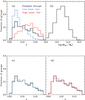 |
Fig. 1 Panel a) shows the spectroscopic redshift distribution of our samples of CGs (black line), and LGs with Ngal ≤ 6 in two ranges of virial mass: low mass (blue line) and high mass (red line). Panel b) shows the virial mass distribution of LGs groups with Ngal ≤ 6 and 0.06 ≤ z ≤ 0.18. Panels c) and d) show the CG redshift distribution (black line), and the low-mass (blue line) and high-mass (red line) subsamples of LGs restricted to have redshift distributions similar to that of the CGs by using a Monte Carlo algorithm (see text for details). |
2. The samples
2.1. The sample of compact groups
The sample of CGs used in this paper was drawn from the catalogue of CGs identified by McConnachie et al. (2009). This catalogue was identified in the public release of the SDSS DR6 (Adelman-McCarthy et al. 2008). McConnachie et al. (2009) used the original selection criteria of Hickson (1982), which defined a CG as a group of galaxies with projected properties such that: the number of galaxies within 3 mag of the brightest galaxies is N(Δm = 3) ≥ 4; the combined surface brightness of these galaxies is μ ≤ 26.0 mag arcsec-2, where the total flux of the galaxies is averaged over the smallest circle that contains their geometric centres and has an angular diameter θG; and θN ≥ 3θG, where θN is the angular diameter of the largest concentric circle that contains no additional galaxies in this magnitude range or brighter.
McConnachie et al. (2009) identified 2297 CGs, adding up to 9713 galaxies down to a Petrosian (Petrosian 1976) limiting magnitude of r = 18 (catalogue A), and 74 791 CGs (313 508 galaxies) down to a limiting magnitude of r = 21 (catalogue B). According to the authors, contamination due to gross photometric errors was removed from the catalogue A through the visual inspection of all galaxy members, and they estimated it is present in the catalogue B at a 14% level. The catalogue A, which we use in this paper as a primary data source, has spectroscopic information for 4131 galaxies (43% completeness). This catalogue includes groups that have a maximum line-of-sight velocity difference smaller than 1000 km s-1 only, to remove interlopers. The median redshift of the groups in this catalogue is zmed = 0.09. In this work, we use a subsample of the catalogue A of McConnachie et al. (2009), restricted to CGs in the redshift range 0.06 ≤ z ≤ 0.18, which have spectroscopic redshifts for at least one member galaxy, and also restricted our analyses to galaxy members with apparent magnitudes 14.5 ≤ r ≤ 17.77, i.e., the range in which the Main Galaxy Sample (MGS; Strauss et al. 2002) is complete. After meeting all these conditions, our group sample comprises 846 CGs adding up to 2270 galaxies, among which, 1310 galaxies (~58%) have measured redshifts. We show in panel (a) of Fig. 1 the redshift distribution of the CGs in our sample. For every galaxy in the CGs with no redshift information, we assumed that its redshift is the parent group’s redshift.
2.2. The sample of loose groups
The loose groups of galaxies used in this paper are groups identified in redshift space, and are not required to fulfil any compactness or isolation criterion. In particular, we use groups drawn from the sample of Zandivarez & Martínez (2011) identified in the MGS of the seventh data release (DR7, Abazajian et al. 2009). Briefly, they used a friends-of-friends algorithm (Huchra & Geller 1982) to link MGS galaxies into groups. This is followed by a second identification using a higher density contrast in groups with at least 10 members, in order to split merged systems and clean up any spurious member detection. Given the known sampling problems for bright galaxies, the group identification was carried out over all MGS galaxies with 14.5 ≤ r ≤ 17.77. Group virial masses were computed as M = σ2Rvir/G, where Rvir is the virial radius of the system and σ is the velocity dispersion of member galaxies (Limber & Mathews 1960). The velocity dispersion was estimated using the line-of-sight velocity dispersion σv,  . The computation of σv was carried out using the methods described by Beers et al. (1990), by applying the biweight estimator for groups with more than 15 member and the gapper estimator for poorer systems. The sample of Zandivarez & Martínez (2011, hereafter ZM11) comprises 15 961 groups with more than 4 members, adding up to 103 342 galaxies. Groups in this sample have a mean velocity dispersion of 193 km s-1, a mean virial mass of 2.1 × 10¹³ h-1 M⊙, and a mean virial radius of 0.9 h-1 Mpc. We refer the reader to ZM11 for details of the identification procedure and parameters.
2.2.1. The high and low mass subsamples
Since our work intends to perform a fair comparison between the galaxies inhabiting CGs and LGs we do not use the groups of the ZM11 sample in a straightforward way. It is well-known that the properties of galaxies in groups are correlated with group mass (e.g. Martínez & Muriel 2006), thus, in our analyses below we compare galaxies in the CGs with galaxies in LGs in different mass ranges. We divide the groups in the ZM11 sample into two subsamples of low, log (M/M⊙ h-1) ≤ 13.2, and high, log (M/M⊙ h-1) ≥ 13.6, mass. These two subsamples have different redshift distributions, that also differ from that of the CGs, as can be seen in the panel (a) of Fig. 1. Thus, a direct comparison between the galaxies in these two subsamples and the CGs will certainly be biased. We then use a Monte Carlo algorithm to randomly select groups from these two subsamples in order to construct new subsamples of low and high mass LGs that have redshift distributions similar to that of the CGs. In panels (c) and (d) of Fig. 1, we show the resulting redshift distributions and the redshift distribution of the CGs as a comparison. A Kolmogorov-Smirnov test (KS) comparing these distributions with that of the CGs gives significance levels for the null hypothesis that they are drawn from the same distribution above of 95%. Our final subsamples of low and high mass LGs include 2536 and 2529 systems, adding up to 8749 and 10 055 galaxies, respectively.
2.2.2. The equal luminosity subsamples of compact and loose groups
We would ideally like to compare galaxies in LGs and CGs of similar masses, which cannot be done since CGs in the McConnachie et al. (2009) catalogues do not have measured masses. Another way of comparing CGs and LGs that have similar characteristics can be done by selecting them according to the total luminosity of their galaxy members. Thus, we also perform a comparison of galaxy properties in samples of CGs and LGs with similar luminosity distributions. The luminosities of our LGs were computed by Martínez & Zandivarez (2012) using the method of Moore et al. (1993), which accounts for the galaxy members not observed owing to the apparent magnitude limit by considering the luminosity function (LF) of galaxies in groups. Martínez & Zandivarez (2012) used the mass-dependent LF of ZM11.
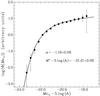 |
Fig. 2 The luminosity function of galaxies in compact groups. Continuous line is the best-fit Schechter function with shape parameters quoted inside the figure. These parameters are used to compute the luminosities of CGs. |
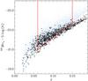 |
Fig. 3 The 0.1r-band group absolute magnitude (GRM0.1r) as a function of redshift. Light blue dots are the LGs, and open black circles are the CGs. We show in red lines the region of the diagram within which we select subsamples of LGs and CGs restricted to have similar redshift and absolute magnitude distributions. |
To compute the total luminosities of the CGs using the method of Moore et al. (1993), we need first to compute the LF of the galaxies in CGs. We use two methods to compute the LF of galaxies in CGs: the non-parametric C − (Lynden-Bell 1971; Choloniewski 1987) for the binned LF and the STY method (Sandage et al. 1979) to compute the best-fit Schechter (1976) function parameters. Since the catalogue A of McConnachie et al. (2009) is complete down to an apparent magnitude r = 18, we included all galaxies brighter than this limit in the LF computation. We show in Fig. 2 the resulting LF of galaxies in CGs in the 0.1r-band. The best-fit Schechter function has shape parameters α = −1.19 ± 0.06 and M∗ − 5log (h) = −21.21 ± 0.08 and is clearly a good fit to the C − points. It is interesting to compare these LF parameters with those found by ZM11 for the catalogue of LGs used in this paper. On the one hand, the M∗ is comparable with the value − 21.18 ± 0.04 that ZM11 found for their highest mass bin, that is, groups with masses in the range 1.5−3.0 × 10¹⁴ M⊙ h-1. On the other hand, the faint-end slope value is consistent with the value −1.19 ± 0.04 corresponding to LGs of intermediate mass ~3.5 × 10¹³ M⊙ h-1 in ZM11.
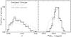 |
Fig. 4 Redshift (left panel) and total group absolute magnitude (right panel) distributions of groups in the region defined in Fig. 3: CGs (black), LGs (light blue) and LGs selected by a Monte Carlo algorithm to ensure that their redshift, and absolute magnitude distributions are similar to those of the CGs (grey). |
We show in Fig. 3 the absolute magnitude of LGs and CGs as a function of redshift. Clear differences are observed between LGs and CGs: at a fixed redshift, the brightest objects are LGs and the faintest are CGs. Among the LGs, there are systems which can have more members than typical CGs and that are thus brighter. Compact groups were identified over a parent catalogue that has a fainter apparent-magnitude limit (r = 18) than the MGS (r = 17.77), which is the parent catalogue for the LGs of ZM11. This explains why there are CGs much fainter than even the faintest LGs, particularly at z > 0.15.
To perform a fair comparison between LGs and CGs having similar absolute-magnitude distributions, we firstly define a region in the redshift-absolute magnitude plane in which we can find both types of groups. As discussed above, for all redshifts z > 0.05, the CG sample includes systems that are fainter than all the LGs owing to differences in the apparent magnitude limit of the parent catalogues. As can be seen in Fig. 3, beyond z > 0.15 the samples of LGs and CGs do not overlap at all, this imposes the upper redshift cut-off. For the lower redshift cut-off, we use the same value, z = 0.06, as in the other samples defined before. Within this redshift range, we avoid the region in which only CGs are found, that is, we impose a redshift-dependent faint absolute magnitude cut-off that, for simplicity, we have chosen to be linear. We indicate this region with red lines in Fig. 3. Within this region, LGs and CGs have different redshift and absolute magnitude distributions, which we show in Fig. 4 as black and light blue histograms, respectively. We then select by means of a Monte Carlo algorithm, a subsample of LGs that match the redshift and absolute magnitude distributions of the CGs. This is shown as grey histograms in Fig. 4. When we compare LGs and CGs of equal luminosity in the analyses below, we refer to these two subsamples of groups. Our final subsamples of EQL-CGs and EQL-LGs include 571 and 2345 systems, adding up to 1729 and 10 554 galaxies, respectively. We explicitly make this distinction between the CG and the EQL-CG samples since the latter has a redshift-dependent absolute-magnitude constraint that is absent in the former.
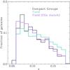 |
Fig. 5 Redshift distributions of galaxies: CGs sample (black), field galaxies (green), and field galaxies selected by using a Monte Carlo algorithm to have a similar redshift distribution as CGs (violet). |
2.3. The sample of field galaxies
We also compare the properties of galaxies in CGs with the properties of field galaxies. We consider as field galaxies all DR7 MGS galaxies that were not identified as belonging to LGs by ZM11 groups or to CGs by McConnachie et al. (2009), with apparent magnitudes 14.5 ≤ r ≤ 17.77. For an adequate comparison with our samples of galaxies in groups, we used the same Monte Carlo algorithm of the previous subsection to contract a sample of field galaxies that has a similar redshift distribution as that of galaxies in our CG sample. This field sample includes 250 725 galaxies. We show in Fig. 5 the redshift distributions of galaxies in CGs, of all field galaxies and field galaxies that were Monte Carlo selected. A KS test between the galaxies in CGs and in our Monte Carlo selected field samples gives significance levels for the null hypothesis that they are drawn from the same distribution above of 95%. From now on, when we refer to field galaxies we mean galaxies in this Monte Carlo selected sample.
3. Comparing galaxies in CGs, LGs, and in the field
We compare parameters of galaxies in CGs, LGs, and in the field. The parameters on which we focus our study are:
-
Petrosian absolute magnitude in the 0.1r-band.
-
The radius that encloses 50% of the Petrosian flux r50.
-
The r-band surface brightness, μ50, computed inside r50.
-
The concentration index, defined as the ratio of the radii enclosing 90 and 50 percent of the Petrosian flux, C = r90/r50.
-
The 0.1(u − r) colour. We use model instead of Petrosian magnitudes to compute colours since aperture photometry may include non-negligible Poisson and background subtraction uncertainties in the u band.
-
The stellar mass, M∗ based on luminosity and colour, computed following Taylor et al. (2011).
In the analyses below, we classify galaxies into early and late types according to their concentration index. Early-type galaxies typically have C > 2.5, while for late-types C < 2.5 (Strateva et al. 2001). The effects of seeing in the measurement of r50 and r90 have to be considered for galaxies with relatively small angular sizes. The average seeing in the SDSS is below a conservative value of 1.5′′ (Shen et al. 2003). Since the values of r50, μ50, and C can be unreliable for galaxies with r50 below this value, we excluded them from our analyses. The numbers of galaxies in each sample quoted in the previous section are based on this size cut-off.
Since many galaxy properties correlate with absolute magnitude, to perform a fair comparison we weight each galaxy in our computations by 1/Vmax (Schmidt 1968) in order to compensate for our dealing with galaxy samples that are drawn from flux-limited catalogues. Figure 6 compares the normalised distributions of galaxy parameters of galaxies in LGs and the field with those of CG galaxies. Below each panel of Fig. 6, we show the residuals between each pair of distributions, i.e., for each property X, the difference ΔF(X) = fCG(X) − f(X), where fCG(X) and f(X) are the fractions of galaxies in the bin centred on X in the CG and the other sample, respectively.
In terms of luminosity, and as can be seen from Fig. 6, galaxies in CGs tend to be slightly more luminous than their field counterparts, in the sense of an excess of M0.1r − 5log (h) ≲ − 20 galaxies, which agrees with the previous findings of Deng et al. (2008). We find no clear difference from either low or high mass LGs. A similar result is found by Deng et al. (2007) when comparing galaxies in CGs and LGs identified by different algorithms. Important differences can be seen between CGs and the sample of LGs restricted to have similar total luminosity distributions (hereafter EQL-LG): galaxies in CGs are systematically brighter.
Compared to all LG samples and the field, CGs have a larger fraction of galaxies with μ50 ≲ 20.4 mag arcsec-2 and a deficit of lower surface-brightness galaxies.
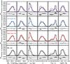 |
Fig. 6 Distributions of galaxy properties in our samples: CGs sample (thick black line), field (violet), low-mass LGs (blue), high-mass LGs (red), and EQL-LG (thin black line). All distributions have been normalised to have the same area. Below each panel, we show as shaded histograms the residuals between the distributions. |
When comparing galaxy sizes, we find differences between CGs and the other environments for galaxies with r50 ≲ 3 kpc. Compact groups contain an excess of galaxies with r50 ≲ 2 kpc and a deficit of 2 kpc ≲ r50 ≲ 3 kpc galaxies. Deng et al. (2008) found no significant differences between the sizes of galaxies in CGs and a sample of field galaxies, a result that they argued was due to their narrow luminosity range.
Galaxies in CGs are systematically more concentrated than their counterparts in the field or in LGs. This difference reflects that galaxies in CGs have, on average, smaller sizes and comparable luminosities to galaxies in the other samples. Thus, CGs have a larger fraction of early-type galaxies. In agreement with our results, Deng et al. (2008) found that CGs have a larger fraction of highly concentrated early-type galaxies than the field.
In agreement with their relatively large fraction of early-type galaxies, galaxies in CGs show a larger fraction of red galaxies, than the field and the LGs. Our results agree with the comparison of CGs and field galaxies by Lee et al. (2004) and Deng et al. (2008). Brasseur et al. (2009) arrived at similar results performing a similar comparison using mock catalogues based on the Millennium Run simulation (Springel et al. 2005).
Galaxies in CGs tend to have higher stellar masses than their field and EQL-LGs counterparts. We explore this result further in Fig. 7, where we show the median stellar mass as a function of absolute magnitude for galaxies in all our samples. Differences arise at the lower luminosities that we explore, galaxies in groups differ from field galaxies, being more massive at fixed luminosity. At the same time, something similar is observed when comparing the equal luminosity subsamples: galaxies in CGs appear to be more massive at lower luminosities. All of these differences are almost erased when we consider early types only.
As a general conclusion from this section, galaxies in CGs differ from galaxies in other environments. Differences are larger when compared to field galaxies and smaller when compared to galaxies in high mass LGs.
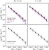 |
Fig. 7 The stellar mass as a function absolute magnitude for galaxies in our samples. Points represent the median in each bin, error-bars are the 25% and 75% percentiles within each bin. |
3.1. The fraction of red and early-type galaxies in groups
As a complementary study, we also study the fraction of galaxies that are in the red sequence or are classified as early-type as a function of galaxy absolute magnitude in the environments that we probe. To quantify the fraction of red galaxies, we follow ZM11 and classify galaxies as red/blue accordingly to whether their 0.1(u − r) colour is larger/smaller than the luminosity dependent threshold T(x) = −0.02x2 − 0.15x + 2.46, where x = M0.1r − 5log (h) + 20. To classify galaxies into early- and late-types, we use the concentration parameter and consider as early types those galaxies that have C > 2.5.
Figure 8 shows the fraction of red galaxies (left panels), early-type galaxies (centre panels), and red early-type galaxies (right panels) as a function of galaxy absolute magnitude. The comparison among CGs, LG samples, and the field shows that CGs have a larger fraction of red early-type galaxies over the whole absolute magnitude range. For brighter luminosities, CGs and high mass LGs have similar fractions of red galaxies, the largest difference being observed when red and early-types galaxies are considered. Important differences can be seen between CGs and LGs of similar luminosities (lower panels).
4. Photometric relations
There are well-known scaling relations involving the photometric, structural, and dynamical parameters of galaxies. Among the scaling relations that involve photometric parameters are the colour − magnitude (Sandage & Visvanathan 1978a,b), also known as the red sequence (RS) for early-type galaxies, and the luminosity-size relation. These empirical relations are closely related to the physical processes involved in the galaxy formation scenario, hence are a fundamental tools in helping us to understand the formation and evolution of galaxies. In this section, we compare these relations for our samples of galaxies in CGs, LGs, and in the field. As in the previous section, we weight each galaxy by 1/Vmax according to its absolute magnitude and the redshift and apparent magnitude cut-offs.
4.1. Colour–magnitude diagram: red sequence
Figure 9 shows the colour − magnitude diagram as a function of environment. As expected, it is clear from the left panels of Fig. 9 that, as we move from field to LGs of increasing mass, the blue population declines in numbers, while red galaxies become the dominant population. For CG the red population is even more dominant. The right panels of Fig. 9 consider only early-type galaxies, since they are selected according to their concentration parameter alone, there is a blue population that has not been completely removed. This blue population becomes less prominent as we move from field to CGs. Lee et al. (2004) and Brasseur et al. (2009) found that galaxies in compact associations are confined nearly exclusively to the red sequence, with few galaxies occupying the blue cloud, in agreement with our results.
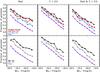 |
Fig. 8 Left panels: the fraction of red galaxies according to their 0.1(u − r) colour; centre panels: the fraction of early-type galaxies according to their concentration parameter; right panels: the fraction of red early-type galaxies. All fractions are shown as a function of absolute magnitude. The upper panels compare CGs, LGs of low and high mass, and field galaxies, while lower panels compare CGs and LGs with similar redshift and total absolute magnitude. Vertical error-bars are obtained by using the bootstrap resampling technique, horizontal error-bars are the 25% and 75% quartiles of the absolute magnitude distribution within each bin. |
It is well-known that, for a fixed absolute magnitude, M, the colour distribution of the galaxies is well-described by the sum of two Gaussian functions representing the blue cloud and the red sequence (e.g. Baldry et al. 2004; Balogh et al. 2004; Martínez et al. 2006)  (1)In the equation above, AB and AR are the amplitudes, μB and μR the centres, and σB and σR the width of the Gaussian functions describing the blue (B) and red (R) populations. We study the environmental dependence of the red sequence following the same procedure as in Martínez et al. (2010): for different absolute magnitude bins, we fit the two Gaussian model (Eq. (1)) to the 0.1(u − r) colour distribution of field, LG, and CG galaxies, using a standard Levenberg-Marquardt method. Thus, for all our galaxy samples we have the six parameters of Eq. (1) as a function of 0.1r-band absolute magnitude. In Fig. 10, we show the centre of the Gaussian function (μR) that most closely fits the red sequence in the colour − magnitude diagrams of Fig. 9. The abscissas are the medians of the corresponding distributions of the absolute magnitudes in each bin and the horizontal error bars are the 25% and 75% quartiles.
In the absolute magnitude range that we probe in this work, we find that data points in Fig. 10 are well-described by a quadratic polynomial (Martínez et al. 2010). The continuous lines in Fig. 10 show the best quadratic fits to μR as a function of the absolute magnitude. This figure shows (upper left panel) that the red sequence of field galaxies is always bluer than its counterparts in groups. Among groups, the mean colour of the red sequence is systematically redder for the high mass subsample (as in Martínez et al. 2010). The μR of CG galaxies agrees with that of galaxies in high mass LGs over the whole range of absolute magnitudes that we probe. When considering the samples of CGs and LGs of similar luminosities (lower left panel), the μR of CGs is systematically redder for M0.1r − 5log (h) < −20.5. When we consider red early-type galaxies alone (right panels of Fig. 10), the differences between our results for the field, LGs, and CGs disappear. Nevertheless, differences between the red sequences of CGs, LGs, and the field are still present.
4.2. Luminosity-size relation
Figure 11 shows the Petrosian half-light radius as a function of absolute magnitude of late (lefts panels) and early-type galaxies (right panels). As expected, brighter galaxies are larger, as previously found in several environments independently of the morphological types (e.g. Coenda et al. 2005; Bernardi et al. 2007; von der Linden et al. 2007; Coenda & Muriel 2009; Nair et al. 2010).
To analyse the luminosity-size relation, for each panel in Fig. 11, we derive the size distribution within several absolute magnitude bins. In all cases, for a fixed absolute magnitude, M, the size (r50) distribution can be well-described by a log-normal distribution (Shen et al. 2003), which is characterised by a median (μ = ln(rmed)) and a dispersion (σ)  (2)We fit this model to the distributions shown in Fig. 11 using a standard Levenberg-Marquardt procedure. Figure 12 shows the median log (rmed) as a function of the absolute magnitude of the distributions shown in Fig. 11. For all samples of galaxies analysed here, a quadratic polynomial function is a good description of the median log (rmed) as a function of absolute magnitude. We also show these fits in Fig. 12. The curvature in the luminosity-size relation was previously reported by Bernardi et al. (2007) and Coenda & Muriel (2009).
Taking into account the error-bars, the differences among the different sequences in Fig. 12 are insignificant for most of the bins. The only clear difference is seen between early-type galaxies populating the EQL CG sample and the field. Nevertheless, a systematic behaviour can be seen in all panels of Fig. 12: over the whole range on luminosities, galaxies in CGs tend to be the smallest, while field galaxies are the largest. This effect is observed for both early and late-type galaxies. Analysing central and satellite galaxies, Weinmann et al. (2009) found a similar dependence of the size-luminosity relation on the environment, although they found that the effect is only observed for late-type galaxies. These authors adopted a more restrictive C > 3 value to select early-type galaxies. This threshold preferentially selects elliptical galaxies. To compare our results with those obtained by Weinmann et al. (2009), we consider a sub-sample of early-type galaxies for which C > 3. The corresponding results are shown in the inset-panels of Fig. 12, where it can be observed that the size-luminosity relation for C > 3 galaxies is the same for all the environments considered. This agrees with Nair et al. (2010), who, by using a sample of visually classified bright sample of galaxies, found no dependence on environment of the size-luminosity relation for elliptical galaxies.
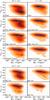 |
Fig. 9 Colour − magnitude diagram: 0.1(u − r) as a function of |

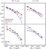 |
Fig. 10 μR of the sequences of red galaxies from Fig. 9 as a function of absolute magnitude. The abscissas are the median and the horizontal error bars are the 25% and 75% quartiles of the absolute magnitude distribution within each luminosity bin. Vertical error bars are the 1σ error estimates from the fitting procedure. Continuous lines are the best-fit quadratic models. |
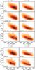 |
Fig. 11 Petrosian half-light radius, r50, as function of the absolute magnitude for field and both low and high mass LG and CG galaxies. Equal luminosity samples of CGs and LGs are shown separately. Left panels show late-type galaxies, while right panels consider early-type galaxies according to their concentration parameter. |
5. Conclusions and discussion
To investigate the dependence of the galaxy properties on environment, we have performed a comparative study of the properties of galaxies in CGs, LGs, and in the field in the redshift range 0.06 < z < 0.18. Compact groups analysed in this paper were drawn from the catalogue A of McConnachie et al. (2009), while LGs were selected from the sample of ZM11. In all cases, galaxy properties used in our work were taken from the MGS sample of the SDSS DR7.
We have selected three samples of LGs taken from the ZM11 catalogue, the first two consisting of low (log (M/M⊙ h-1) ≤ 13.2) and high (log (M/M⊙ h-1) ≥ 13.6) mass. The third sample has been selected to ensure that it has a similar total luminosity distribution to that of CGs. Since the original samples of CGs and LGs have different redshift distributions, we constructed the LG group samples by using a Monte Carlo algorithm that randomly selects groups in order to reproduce the redshift distribution of CGs. Our sample of field galaxies was similarly drawn to reproduce the redshift distribution of CG members. The final samples consist of 846, 2536, and 2529 compact, low-mass, high-mass and equal luminosity loose groups, respectively. The corresponding number of member galaxies are 2270, 8749, and 10 055. The equal luminosity subsamples of compact and loose groups include 571 and 2345 objects, adding up to 1729 and 10 554 galaxies, respectively. The field sample comprises 250 725 galaxies. This statistically significant set of data has been used to compare the basic properties of galaxies as well as some photometric scaling relations in different environments.
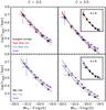 |
Fig. 12 The log (rmed) of the size distribution as a function of absolute magnitude for late-type galaxies (left panels) and early-types galaxies (right panels). The abscissas are the median and the horizontal error bars are the 25% and 75% quartiles of the absolute magnitude distribution within each luminosity bin. Vertical error bars are the 1σ error estimates derived from the fitting procedure. Continuous lines are the best-fit quadratic models. Inset panels show the results of using C > 3 to define early-type galaxies. |
Our main findings are:
-
The properties of galaxies in either LGs or the field do not matchthose of galaxies in CGs.
-
Compact groups are the environment that contains the largest fraction of both early-type and red galaxies (our comparison between CGs and the field agrees with Lee et al. 2004; Deng et al. 2008; Brasseur et al. 2009). This effect is observed for the whole range of absolute magnitude and stellar mass.
-
Galaxies in CGs are, on average, smaller, more compact, and have higher surface brightnesses and stellar masses than in either LGs or the field. Differences are larger when compared to field galaxies and smaller when compared to galaxies in high mass LGs. This disagrees with the previous findings of Deng et al. (2008), but it should be kept in mind that they explored a narrower range in luminosity.
-
The luminosity function of galaxies in CGs has a characteristic magnitude comparable to that of the most massive LGs, while its faint-end slope is similar to that of LGs of intermediate mass (LG luminosity functions measurements by ZM11). These parameters might indicate that the compact group environment is effective in producing bright galaxies and, at the same time, is a more hostile environment for fainter galaxies than LGs. Nevertheless, more solid conclusions on this will only be obtained when the mass measurements of CGs allow a more detailed study of their LF and its dependence on mass.
-
The mean colour of CG galaxies is consistent with that of galaxies in high mass LGs over the whole range of absolute magnitudes that we have probed.
-
For a fixed luminosity and over the whole range of absolute magnitudes, both late- and early-type galaxies in CGs are smaller in size than those in EQL groups and the field. A similar trend is observed when we compared our results for CG galaxies with those of galaxies in low mass groups, although it is statistically insignificant. If early-type galaxies are selected using C > 3, the corresponding size-luminosity relations are environment-independent, in agreement with Weinmann et al. (2009), Nair et al. (2010), and Maltby et al. (2010).
It should be taken into account that we have excluded from our analyses galaxies with r50 smaller than the average seeing in SDSS images. While this avoids introducing any systematics due to the seeing, it also excludes increasingly larger galaxies as we go from the lowest to the highest redshift considered in this work. Thus, the actual differences between galaxies in the different environments probed here might be more significant.
Our results did not significantly change when we: (i) considered only galaxies with spectroscopic redshift in CGs; (ii) restricted our analyses to CGs with higher surface brightnesses. We refer the reader to Appendix A for more details.
One of our most important results is that of galaxies in CGs tend to be more compact, redder, and have higher surface brightnesses than their LG or field counterparts. These galaxies could be the descendants of galaxies that inhabited LGs before going through a GC phase. In the CG environment, galaxies have undergone mergers and tidal effects caused by the high densities and small velocity dispersions that characterise CGs. This agrees with the large number of CGs that contain clear examples of galaxies with disturbed morphologies (e.g. Mendes de Oliveira & Hickson 1994). The large fraction of red galaxies in CGs suggests that the aforementioned processes are efficient in producing objects with earlier morphological types. This large fraction of red galaxies in CGs provides additional evidence of an advanced stage of the morphological transformation processes, which is consistent with the predictions of the numerical simulations of Brasseur et al. (2009), who conclude that galaxies in CGs should be mainly red and dead ellipticals. Our results are also consistent with previous studies of the galaxy SFR in compact groups, such as Walker et al. (2010) and Tzanavaris et al. (2010). The differences between the luminosity function of galaxies in CGs and LGs also support a scenario where low luminosity galaxies merge efficiently leading to both a smaller number of faint galaxies and larger number of bright early-type galaxies, as observed.
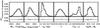 |
Fig. A.1 Distributions of galaxy properties of CGs: whole sample (thick line) and members with spectroscopic redshifts (thin line). |
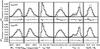 |
Fig. A.2 Distributions of galaxy properties of CGs with μ ≤ 26.0 mag arcsec-2 (thick line), μ ≤ 25.0 mag arcsec-2, and μ ≤ 24.0 mag arcsec-2 (thin line). |
Recent results (e.g. Cortese et al. 2006; Wilman et al. 2009), McGee et al. (2009) suggest that groups of galaxies play a fundamental role in the pre-processing of galaxies before they become part of more massive systems such as clusters of galaxies. Our results indicate that galaxies that inhabit a high density environment, such as CGs, have undergone a major transformation compared to objects that presently occupy a LG. Within this scenario, the properties of galaxies in high mass systems such as clusters, should display considerable variations in their galaxy properties depending on the fraction of members that have undergone a CG phase.
Acknowledgments
We thank the anonymous referee for useful comments and suggestion that improved the paper. This work was supported with grants from CONICET (PIP 11220080102603 and 11220100100336), Ministerio de Ciencia y Tecnología (PID 2008/14797627), Provincia de Córdoba, and SECYT-UNC, Argentina. Funding for the Sloan Digital Sky Survey (SDSS) has been provided by the Alfred P. Sloan Foundation, the Participating Institutions, the National Aeronautics and Space Administration, the National Science Foundation, the US Department of Energy, the Japanese Monbukagakusho, and the Max Planck Society. The SDSS Web site is http://www.sdss.org/. The SDSS is managed by the Astrophysical Research Consortium (ARC) for the Participating Institutions. The Participating Institutions are The University of Chicago, Fermilab, the Institute for Advanced Study, the Japan Participation Group, The Johns Hopkins University, the Korean Scientist Group, Los Alamos National Laboratory, the Max Planck Institut für Astronomie (MPIA), the Max Planck Institut für Astrophysik (MPA), New Mexico State University, University of Pittsburgh, University of Portsmouth, Princeton University, the United States Naval Observatory, and the University of Washington.
References
- Abadi, M. G., Moore, B., & Bower, R. G. 1999, MNRAS, 308, 947 [NASA ADS] [CrossRef] [Google Scholar]
- Abazajian, K. N., Adelman-McCarthy, J. K., Agüeros, M. A., et al. 2009, ApJS, 182, 543 [NASA ADS] [CrossRef] [Google Scholar]
- Adelman-McCarthy, J. K., Agüeros, M. A., Allam, S. S., et al. 2008, ApJS, 175, 297 [NASA ADS] [CrossRef] [Google Scholar]
- Baldry, I. K., Glazebrook, K., Brinkmann, J., et al. 2004, ApJ, 600, 681 [NASA ADS] [CrossRef] [Google Scholar]
- Balogh, M. L., Navarro, J. F., & Morris, S. L. 2000, ApJ, 540, 113 [NASA ADS] [CrossRef] [Google Scholar]
- Balogh, M. L., Baldry, I. K., Nichol, R., et al. 2004, ApJ, 615, L101 [NASA ADS] [CrossRef] [Google Scholar]
- Beers, T. C., Flynn, K., & Gebhardt, K. 1990, AJ, 100, 32 [NASA ADS] [CrossRef] [Google Scholar]
- Bernardi, M. 2009, MNRAS, 510 [Google Scholar]
- Bernardi, M., Hyde, J. B., Sheth, R. K., Miller, C. J., & Nichol, R. C. 2007, AJ, 133, 1741 [NASA ADS] [CrossRef] [Google Scholar]
- Bitsakis, T., Charmandaris, V., Le Floc’h, E., et al. 2010, A&A, 517, A75 [NASA ADS] [CrossRef] [EDP Sciences] [Google Scholar]
- Blanton, M. R., Brinkmann, J., Csabai, I., et al. 2003, AJ, 125, 2348 [NASA ADS] [CrossRef] [Google Scholar]
- Blanton, M. R., Eisenstein, D., Hogg, D. W., Schlegel, D. J., & Brinkmann, J. 2005, ApJ, 629, 143 [NASA ADS] [CrossRef] [Google Scholar]
- Brasseur, C. M., McConnachie, A. W., Ellison, S. L., & Patton, D. R. 2009, MNRAS, 392, 1141 [NASA ADS] [CrossRef] [Google Scholar]
- Choloniewski, J. 1987, MNRAS, 226, 273 [NASA ADS] [CrossRef] [Google Scholar]
- Coenda, V., & Muriel, H. 2009, A&A, 504, 347 [NASA ADS] [CrossRef] [EDP Sciences] [Google Scholar]
- Coenda, V., Donzelli, C. J., Muriel, H., et al. 2005, AJ, 129, 1237 [NASA ADS] [CrossRef] [Google Scholar]
- Colless, M., Dalton, G., Maddox, S., et al. 2001, MNRAS, 328, 1039 [NASA ADS] [CrossRef] [Google Scholar]
- Cortese, L., Gavazzi, G., Boselli, A., et al. 2006, A&A, 453, 847 [Google Scholar]
- Deng, X.-F., He, J.-Z., & Jiang, P. 2007, ApJ, 671, L101 [NASA ADS] [CrossRef] [Google Scholar]
- Deng, X.-F., He, J.-Z., & Wu, P. 2008, A&A, 484, 355 [NASA ADS] [CrossRef] [EDP Sciences] [Google Scholar]
- Diaferio, A., Geller, M. J., & Ramella, M. 1994, AJ, 107, 868 [NASA ADS] [CrossRef] [Google Scholar]
- Díaz-Giménez, E., & Mamon, G. A. 2010, MNRAS, 409, 1227 [NASA ADS] [CrossRef] [Google Scholar]
- Dressler, A. 1980, ApJS, 42, 565 [NASA ADS] [CrossRef] [Google Scholar]
- Eke, V. R., Baugh, C. M., Cole, S., et al. 2004, MNRAS, 348, 866 [NASA ADS] [CrossRef] [Google Scholar]
- Gerke, B. F., Newman, J. A., Faber, S. M., et al. 2007, MNRAS, 376, 1425 [NASA ADS] [CrossRef] [Google Scholar]
- Goto, T., Yamauchi, C., Fujita, Y., et al. 2003, MNRAS, 346, 601 [NASA ADS] [CrossRef] [Google Scholar]
- Gunn, J. E., & Gott, J. R. I. 1972, ApJ, 176, 1 [NASA ADS] [CrossRef] [Google Scholar]
- Hansen, S. M., Sheldon, E. S., Wechsler, R. H., & Koester, B. P. 2009, ApJ, 699, 1333 [NASA ADS] [CrossRef] [Google Scholar]
- Hickson, P. 1982, ApJ, 255, 382 [NASA ADS] [CrossRef] [Google Scholar]
- Hickson, P., Mendes de Oliveira, C., Huchra, J. P., & Palumbo, G. G. 1992, ApJ, 399, 353 [NASA ADS] [CrossRef] [EDP Sciences] [MathSciNet] [PubMed] [Google Scholar]
- Huchra, J. P., & Geller, M. J. 1982, ApJ, 257, 423 [NASA ADS] [CrossRef] [Google Scholar]
- Iovino, A., de Carvalho, R. R., Gal, R. R., et al. 2003, AJ, 125, 1660 [NASA ADS] [CrossRef] [Google Scholar]
- Johnson, K. E., Hibbard, J. E., Gallagher, S. C., et al. 2007, AJ, 134, 1522 [NASA ADS] [CrossRef] [Google Scholar]
- Kawata, D., & Mulchaey, J. S. 2008, ApJ, 672, L103 [Google Scholar]
- Larson, R. B., Tinsley, B. M., & Caldwell, C. N. 1980, ApJ, 237, 692 [NASA ADS] [CrossRef] [Google Scholar]
- Lee, B. C., Allam, S. S., Tucker, D. L., et al. 2004, AJ, 127, 1811 [NASA ADS] [CrossRef] [Google Scholar]
- Limber, D. N., & Mathews, W. G. 1960, ApJ, 132, 286 [NASA ADS] [CrossRef] [Google Scholar]
- Lynden-Bell, D. 1971, MNRAS, 155, 95 [NASA ADS] [CrossRef] [Google Scholar]
- Maltby, D. T., Aragón-Salamanca, A., Gray, M. E., et al. 2010, MNRAS, 402, 282 [NASA ADS] [CrossRef] [Google Scholar]
- Martínez, H. J., & Muriel, H. 2006, MNRAS, 370, 1003 [NASA ADS] [CrossRef] [Google Scholar]
- Martínez, H. J., & Zandivarez, A. 2012, MNRAS, 419, L24 [Google Scholar]
- Martínez, H. J., Zandivarez, A., Merchán, M. E., & Domínguez, M. J. L. 2002, MNRAS, 337, 1441 [NASA ADS] [CrossRef] [Google Scholar]
- Martínez, H. J., O’Mill, A. L., & Lambas, D. G. 2006, MNRAS, 372, 253 [NASA ADS] [CrossRef] [Google Scholar]
- Martínez, H. J., Coenda, V., & Muriel, H. 2010, MNRAS, 403, 748 [NASA ADS] [CrossRef] [Google Scholar]
- McConnachie, A. W., Ellison, S. L., & Patton, D. R. 2008, MNRAS, 387, 1281 [NASA ADS] [CrossRef] [Google Scholar]
- McConnachie, A. W., Patton, D. R., Ellison, S. L., & Simard, L. 2009, MNRAS, 395, 255 [NASA ADS] [CrossRef] [Google Scholar]
- McGee, S. L., Balogh, M. L., Bower, R. G., Font, A. S., & McCarthy, I. G. 2009, MNRAS, 400, 937 [NASA ADS] [CrossRef] [Google Scholar]
- McGee, S. L., Balogh, M. L., Wilman, D. J., et al. 2011, MNRAS, 413, 996 [NASA ADS] [CrossRef] [Google Scholar]
- Mendel, J. T., Ellison, S. L., Simard, L., Patton, D. R., & McConnachie, A. W. 2011, MNRAS, 418, 1409 [NASA ADS] [CrossRef] [Google Scholar]
- Mendes de Oliveira, C., & Hickson, P. 1994, ApJ, 427, 684 [NASA ADS] [CrossRef] [Google Scholar]
- Merchán, M., & Zandivarez, A. 2002, MNRAS, 335, 216 [NASA ADS] [CrossRef] [Google Scholar]
- Merchán, M. E., & Zandivarez, A. 2005, ApJ, 630, 759 [NASA ADS] [CrossRef] [Google Scholar]
- Moore, B., Frenk, C. S., & White, S. D. M. 1993, MNRAS, 261, 827 [NASA ADS] [Google Scholar]
- Moore, B., Lake, G., & Katz, N. 1998, ApJ, 495, 139 [NASA ADS] [CrossRef] [Google Scholar]
- Nair, P. B., van den Bergh, S., & Abraham, R. G. 2010, ApJ, 715, 606 [NASA ADS] [CrossRef] [Google Scholar]
- Oemler, A. J. 1974, ApJ, 194, 1 [NASA ADS] [CrossRef] [Google Scholar]
- Petrosian, V. 1976, ApJ, 209, L1 [NASA ADS] [CrossRef] [Google Scholar]
- Rasmussen, J., Ponman, T. J., Verdes-Montenegro, L., Yun, M. S., & Borthakur, S. 2008, MNRAS, 388, 1245 [NASA ADS] [CrossRef] [Google Scholar]
- Sandage, A., & Visvanathan, N. 1978a, ApJ, 225, 742 [NASA ADS] [CrossRef] [Google Scholar]
- Sandage, A., & Visvanathan, N. 1978b, ApJ, 223, 707 [NASA ADS] [CrossRef] [Google Scholar]
- Sandage, A., Tammann, G. A., & Yahil, A. 1979, ApJ, 232, 352 [NASA ADS] [CrossRef] [EDP Sciences] [Google Scholar]
- Schechter, P. 1976, ApJ, 203, 297 [Google Scholar]
- Schlegel, D. J., Finkbeiner, D. P., & Davis, M. 1998, ApJ, 500, 525 [NASA ADS] [CrossRef] [Google Scholar]
- Schmidt, M. 1968, ApJ, 151, 393 [NASA ADS] [CrossRef] [Google Scholar]
- Shen, S., Mo, H. J., White, S. D. M., et al. 2003, MNRAS, 343, 978 [NASA ADS] [CrossRef] [Google Scholar]
- Springel, V., White, S. D. M., Jenkins, A., et al. 2005, Nature, 435, 629 [NASA ADS] [CrossRef] [PubMed] [Google Scholar]
- Strateva, I., Ivezić, Ž., Knapp, G. R., et al. 2001, AJ, 122, 1861 [Google Scholar]
- Strauss, M. A., Weinberg, D. H., Lupton, R. H., et al. 2002, AJ, 124, 1810 [NASA ADS] [CrossRef] [Google Scholar]
- Taylor, E. N., Hopkins, A. M., Baldry, I. K., et al. 2011, MNRAS, 418, 1587 [NASA ADS] [CrossRef] [Google Scholar]
- Toomre, A., & Toomre, J. 1972, ApJ, 178, 623 [NASA ADS] [CrossRef] [Google Scholar]
- Torres-Flores, S., Mendes de Oliveira, C., de Mello, D. F., et al. 2009, A&A, 507, 723 [NASA ADS] [CrossRef] [EDP Sciences] [Google Scholar]
- Tovmassian, H., Plionis, M., & Torres-Papaqui, J. P. 2006, A&A, 456, 839 [NASA ADS] [CrossRef] [EDP Sciences] [Google Scholar]
- Tzanavaris, P., Hornschemeier, A. E., Gallagher, S. C., et al. 2010, ApJ, 716, 556 [NASA ADS] [CrossRef] [Google Scholar]
- von der Linden, A., Best, P. N., Kauffmann, G., & White, S. D. M. 2007, MNRAS, 379, 867 [NASA ADS] [CrossRef] [Google Scholar]
- Walker, L. M., Johnson, K. E., Gallagher, S. C., et al. 2010, AJ, 140, 1254 [NASA ADS] [CrossRef] [Google Scholar]
- Weinmann, S. M., van den Bosch, F. C., Yang, X., & Mo, H. J. 2006, MNRAS, 366, 2 [NASA ADS] [CrossRef] [Google Scholar]
- Weinmann, S. M., Kauffmann, G., van den Bosch, F. C., et al. 2009, MNRAS, 394, 1213 [NASA ADS] [CrossRef] [Google Scholar]
- Wetzel, A. R., Tinker, J. L., & Conroy, C. 2012, MNRAS, in press [arXiv:1107.5311] [Google Scholar]
- Wilman, D. J., Oemler, Jr., A., Mulchaey, J. S., et al. 2009, ApJ, 692, 298 [NASA ADS] [CrossRef] [Google Scholar]
- Yang, X., Mo, H. J., van den Bosch, F. C., et al. 2007, ApJ, 671, 153 [NASA ADS] [CrossRef] [Google Scholar]
- York, D. G., Anderson, Jr., J. E., Anderson, S. F., et al. 2000, AJ, 120, 1579 [Google Scholar]
- Zandivarez, A., & Martínez, H. J. 2011, MNRAS, 415, 2553 [NASA ADS] [CrossRef] [Google Scholar]
Appendix A: The compact groups sample: contamination
As explained in Sect. 2, we consider in this work a subsample of the catalogue A of CGs identified by McConnachie et al. (2009), which is limited to the redshift range of 0.06 ≤ z ≤ 0.18 and apparent magnitudes 14.5 ≤ r ≤ 17.77 (2270 galaxies). McConnachie et al. (2009) identified CGs following the criteria of Hickson (1982). In particular, the group surface brightness in the r-band is μ ≤ 26.0 mag arcsec-2. The catalogue A includes 1310 galaxies with measured spectroscopic redshifts (~58%). Figure A.1 compares the normalised distributions of the galaxy parameters for all galaxies in CGs and those with measured spectroscopic redshift. Neither significant nor systematic differences can be observed.
McConnachie et al. (2008) found that selecting CGs with a higher surface brightness threshold, decreases the contamination rate. McConnachie et al. (2009) stated that the level of contamination is negligible for their catalogue A. We checked whether our results are affected by contamination by selecting groups with μ ≤ 25.0 mag arcsec-2 and μ ≤ 24.0 mag arcsec-2, and then comparing the properties of their galaxies with the members of groups for which μ ≤ 26.0 mag arcsec-2. We compare the galaxy properties of groups selected according to these three μ values in Fig. A.2. Although the galaxy properties of CGs seem similar when we consider CGs selected with different groups surface brightness, CGs with μ ≤ 24.0 mag arcsec-2 contain a higher fraction of early-and red galaxies.
All Figures
|
Fig. 1 Panel a) shows the spectroscopic redshift distribution of our samples of CGs (black line), and LGs with Ngal ≤ 6 in two ranges of virial mass: low mass (blue line) and high mass (red line). Panel b) shows the virial mass distribution of LGs groups with Ngal ≤ 6 and 0.06 ≤ z ≤ 0.18. Panels c) and d) show the CG redshift distribution (black line), and the low-mass (blue line) and high-mass (red line) subsamples of LGs restricted to have redshift distributions similar to that of the CGs by using a Monte Carlo algorithm (see text for details). |
| In the text | |
|
Fig. 2 The luminosity function of galaxies in compact groups. Continuous line is the best-fit Schechter function with shape parameters quoted inside the figure. These parameters are used to compute the luminosities of CGs. |
| In the text | |
|
Fig. 3 The 0.1r-band group absolute magnitude (GRM0.1r) as a function of redshift. Light blue dots are the LGs, and open black circles are the CGs. We show in red lines the region of the diagram within which we select subsamples of LGs and CGs restricted to have similar redshift and absolute magnitude distributions. |
| In the text | |
|
Fig. 4 Redshift (left panel) and total group absolute magnitude (right panel) distributions of groups in the region defined in Fig. 3: CGs (black), LGs (light blue) and LGs selected by a Monte Carlo algorithm to ensure that their redshift, and absolute magnitude distributions are similar to those of the CGs (grey). |
| In the text | |
|
Fig. 5 Redshift distributions of galaxies: CGs sample (black), field galaxies (green), and field galaxies selected by using a Monte Carlo algorithm to have a similar redshift distribution as CGs (violet). |
| In the text | |
|
Fig. 6 Distributions of galaxy properties in our samples: CGs sample (thick black line), field (violet), low-mass LGs (blue), high-mass LGs (red), and EQL-LG (thin black line). All distributions have been normalised to have the same area. Below each panel, we show as shaded histograms the residuals between the distributions. |
| In the text | |
|
Fig. 7 The stellar mass as a function absolute magnitude for galaxies in our samples. Points represent the median in each bin, error-bars are the 25% and 75% percentiles within each bin. |
| In the text | |
|
Fig. 8 Left panels: the fraction of red galaxies according to their 0.1(u − r) colour; centre panels: the fraction of early-type galaxies according to their concentration parameter; right panels: the fraction of red early-type galaxies. All fractions are shown as a function of absolute magnitude. The upper panels compare CGs, LGs of low and high mass, and field galaxies, while lower panels compare CGs and LGs with similar redshift and total absolute magnitude. Vertical error-bars are obtained by using the bootstrap resampling technique, horizontal error-bars are the 25% and 75% quartiles of the absolute magnitude distribution within each bin. |
| In the text | |
|
Fig. 9 Colour − magnitude diagram: 0.1(u − r) as a function of |
| In the text | |
|
Fig. 10 μR of the sequences of red galaxies from Fig. 9 as a function of absolute magnitude. The abscissas are the median and the horizontal error bars are the 25% and 75% quartiles of the absolute magnitude distribution within each luminosity bin. Vertical error bars are the 1σ error estimates from the fitting procedure. Continuous lines are the best-fit quadratic models. |
| In the text | |
|
Fig. 11 Petrosian half-light radius, r50, as function of the absolute magnitude for field and both low and high mass LG and CG galaxies. Equal luminosity samples of CGs and LGs are shown separately. Left panels show late-type galaxies, while right panels consider early-type galaxies according to their concentration parameter. |
| In the text | |
|
Fig. 12 The log (rmed) of the size distribution as a function of absolute magnitude for late-type galaxies (left panels) and early-types galaxies (right panels). The abscissas are the median and the horizontal error bars are the 25% and 75% quartiles of the absolute magnitude distribution within each luminosity bin. Vertical error bars are the 1σ error estimates derived from the fitting procedure. Continuous lines are the best-fit quadratic models. Inset panels show the results of using C > 3 to define early-type galaxies. |
| In the text | |
|
Fig. A.1 Distributions of galaxy properties of CGs: whole sample (thick line) and members with spectroscopic redshifts (thin line). |
| In the text | |
|
Fig. A.2 Distributions of galaxy properties of CGs with μ ≤ 26.0 mag arcsec-2 (thick line), μ ≤ 25.0 mag arcsec-2, and μ ≤ 24.0 mag arcsec-2 (thin line). |
| In the text | |
Current usage metrics show cumulative count of Article Views (full-text article views including HTML views, PDF and ePub downloads, according to the available data) and Abstracts Views on Vision4Press platform.
Data correspond to usage on the plateform after 2015. The current usage metrics is available 48-96 hours after online publication and is updated daily on week days.
Initial download of the metrics may take a while.