| Issue |
A&A
Volume 543, July 2012
|
|
|---|---|---|
| Article Number | A150 | |
| Number of page(s) | 20 | |
| Section | Extragalactic astronomy | |
| DOI | https://doi.org/10.1051/0004-6361/201118292 | |
| Published online | 13 July 2012 | |
Ionised gas abundances in barred spiral galaxies⋆,⋆⋆
1 Dpto. de Física Teórica y del Cosmos, University of Granada, Facultad de Ciencias (Edificio Mecenas), 18071 Granada, Spain
e-mail: This email address is being protected from spambots. You need JavaScript enabled to view it.
; This email address is being protected from spambots. You need JavaScript enabled to view it.
2 Instituto Universitario Carlos I de Física Teórica y Computacional, Facultad de Ciencias, 18071 Granada, Spain
e-mail: This email address is being protected from spambots. You need JavaScript enabled to view it.
3 Dpto. Física Teórica, Universidad Autónoma de Madrid, Cantoblanco, 28049 Madrid, Spain
e-mail: This email address is being protected from spambots. You need JavaScript enabled to view it.
Received: 18 October 2011
Accepted: 24 April 2012
Abstract
Aims. This is the third paper of a series devoted to studying the properties of bars from long-slit spectroscopy to understand their formation, evolution, and influence on the evolution of disk galaxies. In this paper, we aim to determine the gas metallicity distribution of a sample of 20 barred early-type galaxies. We compare the nebular and stellar metallicity distributions to attempt to infer the origin of the warm gas.
Methods. We performed long-slit spectroscopy along the bar and obtained metallicities derived using different calibrations. We compare the nebular emission metallicities derived using different semi-empirical methods. We carry out AGN diagnostic diagrams for data at different radii to determine the radius of influence of the AGN and the nature of the galactic nuclei. We then derive the gas metallicities along the bars and compare our results to the distribution of stellar metallicities in the same regions.
Results. Most of the gas emission is centrally concentrated, although 15 galaxies also show emission along the bar. In the central regions, gas oxygen abundances are in the range 12 + log (O/H) = 8.4−9.1. The nebular metallicity gradients are very shallow in the bulge and bar regions. For three galaxies (one of them a low-ionization nuclear emission-line region), the gas metallicities lie well below the stellar ones in the bulge region. These results do not depend on the choice of semi-empirical calibration used to calculate the abundances. We see that the galaxies with the lowest metallicities are those with the largest rotational velocities. Unlike our stellar metallicities, we find no correlation between the nebular abundances and the central velocity dispersion. In most galaxies, the gradient in the gas nebular metallicities in the bulge region is shallower than that for the stellar metallicity.
Conclusions. The presence of gas of significantly lower metallicity than the stellar abundances in three of our galaxies, suggests that the gas has an external origin that fuels the present star formation at the center of some early-type barred galaxies. That the bar/disk nebular metallicities are higher than the central ones might indicate that the gas could be accreted via cooling flows instead of radial accretion from gas sitting in the outer parts of the disk.
Key words: galaxies: abundances / galaxies: evolution / galaxies: spiral
Based on observations obtained at Siding Spring Observatory (RSAA, ANU, Australia) and the INT telescope at the ING, La Palma, Spain.
Figure 11 is available in electronic form at http://www.aanda.org
© ESO, 2012
1. Introduction
With the exception of a few primordial light elements, stellar nucleosynthesis is responsible for the secular metal enrichment in galaxies. The final metallicity distribution within a galaxy is reasonably well-reproduced by chemical evolution models considering the appropriate star formation history together with episodes of gaseous inflow and outflows (e.g. Portinari & Chiosi 1999; Chiappini et al. 2000; Prantzos 2008; Colavitti et al. 2008). However, the metallicity gradients can be futher modified by dynamical processes (e.g., Roskar et al. 2008; Schönric & Binney 2009; Sánchez-Blázquez et al. 2009). It is, therefore, evident that observing how metals are distributed in a galaxy should tightly constrain its evolution. However, the detailed dynamical processes responsible for the modification of the metallicity distribution and their importance remains poorly understood.
In particular, it is unknown, from the observational point of view, the importance that bars might have in producing the metallicity radial mixing. Bars are believed to affect the overall dynamics of the galaxy and are a well-known mechanism to induce secular evolution (Athanassoula 2003; Pfenniger & Friedli 1991). For instance, in a previous study (Pérez & Sánchez-Blázquez 2011, hereinafter, Paper II) we hinted that the bulges of early-type barred galaxies have different stellar enrichment histories from the bulges of their unbarred counterparts (see also Ellison et al. 2011, for a similar conclusion for gas-phase metallicities).
Gas and stars respond to the gravitational potential according to their own nature, viscosity and magnetic fields only being important in the former component. The highly asymmetric bar potential induces differential radial motions. While the gas component, which is highly dissipative, is affected by the gravitational torque of the non-axisymmetric mass component, the stars are mainly affected by orbital mixing. Furthermore, studies of the gas-phase abundances provide present-day snap-shots of the interstellar medium abundance. On the other hand, the study of stellar abundances provide archeological clues as to the formation and evolution of the bar. Therefore, studies of stellar and gas metallicities are of crucial importance to interpret the processes dominating galaxy evolution. It is expected that, if gas were injected into the interstellar medium (ISM) from stellar outputs, it would generally be more metal-rich than if it had an external origin.
Deriving the disk radial distribution of stellar abundances from spectroscopic measurements is difficult owing to the low surface brightness of the disk and the contamination of the absorption lines by emission from ionised gas. Few works have tried to overcome these difficulties and have derived the radial distribution for only a small number of galaxies (e.g. Yoachim & Dalcanton 2008; MacArthur et al. 2009; Sánchez-Blázquez et al. 2011). The stellar metallicity gradients along the bars of the 20 early-type galaxies presented here were derived in previous works (Pérez et al. 2009, hereinafter, Paper I) and provided interesting results about the radial distribution of the stellar parameters in the bar region.
As for the nebular gas-abundance distribution, in most studied spiral galaxies, both barred and unbarred, negative radial metallicity gradients along the disk have been obtained for the gas component (e.g. Bresolin et al. 2009). These gradients seem to be shallower for barred than unbarred galaxies, but steeper for late-types than early-types (Pagel & Edmunds 1981; Alloin et al. 1981; Vila-Costas & Edmunds 1992; Zaritsky et al. 1994). The issue is not closed yet, so work is being done to investigate the variation in the gradient with radius (Bresolin et al. 2009 obtain a steeper gradient in the central part of M83, than in the outer disk, beyond 1.2 R25) as well as in azimuth (Balser et al. 2011, for the Milky Way). Simulations explain the shallower gradient in the outer than inner part of a galaxy based on radial mixing processes associated with a strong bar (e.g. Considere et al. 2000; Zahid & Bresolin 2011; Friedli et al. 1994; Friedli 1999). In this work, we focus on the analysis of the gas metallicity, in the bar region of the galaxies presented in Papers I and II.
Only a few works have considered both nebular and stellar metallicities. A pioneering study was presented by Storchi-Bergmann et al. (1994). They found a strong correlation between stellar and gas metallicity by investigating the correlation between the oxygen abundance in the nebular component, and the absorption-line equivalent width W(CIVλ1550) (as a tracer of stellar metallicity) in a sample of 44 star-forming galaxies. They concluded that galaxies with lower values of metallicity appear to experience instantaneous outbreaks of star formation, but those with higher metallicity are probably undergoing stellar formation. Annibali et al. (2010) estimated the gas abundance gradients in early-type galaxies, comparing these results with their stellar metallicities (Annibali et al. 2007), and concluding that the gas metallicity tends to be lower than the stellar one, particularly at higher metallicities.
In this paper, we present an analysis of the radial oxygen abundance distribution in the bulge and bar regions of a sample of 20 early-type barred galaxies, with and without nuclear activity. The stellar component of this sample was studied in Papers I and II. In Sect. 2, observations and data reduction are described. The method to analyze the spectral lines to estimate their flux is presented in Sect. 3. In Sect. 4, we show the diagnostic diagrams and derive the abundance distributions with different methods. A comparison of the nebular and stellar metallicity gradients is also presented in this section. The results are discussed in Sect. 5.
2. Observations and data reduction
We obtained long-slit spectra along the bar major axis1 for our sample of 20 barred galaxies. The observations were performed in two different runs, with the double beam spectrograph at Siding Spring Observatory (Australia, hereinafter, run1) and the IDS spectrograph at the Isaac Newton Telescope (La Palma, Spain, hereinafter, run2). The observations were described in detail in Paper I. To summarise, spectra for seven galaxies were obtained in the first run, covering a wavelength range from 3892−5815 Å and 5390−7314 Å with a spectral resolution of FHWM ~ 2.2 Å. In spite of this overlap between both of these wavelength ranges, a relative calibration was impossible because the transmission of the dichroic gets as low as 50%, producing data of very low signal-to-noise ratio, and we have no bright lines in this region. In the second run, spectra for 13 galaxies were obtained, covering a wavelength range of 3020−6665 Å with a spectral resolution of ~3 Å (FWHM), but the unvignetted range is 3600−6300 Å.
The seeing size during these observations ranges from 0.6′′ to 1.2′′ at the INT and from 1′′ to 1.5′′ at SSO. The characteristics of the sample were described in Papers I and II. For convenience, Table 1 shows the sample main properties.
Atmospheric dispersion can have important effects on spectrophotometry when the slit position angle differs from the parallactic angle during the observations. This is not so critical in our observations as we observed extended objects (diffuse emission or emission knots with sizes typically a few arcseconds larger than our slit width).
In any case, to be on the safe side, we kept the target airmass below 1.6 during the observations to ensure an atmospheric differential refraction between the lines of [OII]λ3727 Å and [OIII]λ5007 Å that is smaller than 1.5′′ (Filippenko 1982). Differential atmospheric refraction between any other pair of lines involved in the empirical metallicity calibrations used in the paper is always smaller than the differential atmospheric refraction between [OII]λ3727 Å and [OIII]λ5007 Å.
For a few galaxies in which the difference between the bar position angle and the parallactic angle was greater than ≈40 deg, we tried to keep the airmass below 1.3 (which implies a differential atmospheric refraction between [OII]λ3727 Å and [OIII]λ5007 Å of ≈1′′).
The reduction of the two runs was carried out with the package REDUCEME (Cardiel 1999) and IRAF tasks. Standard data reduction procedures (flat-fielding, cosmic ray removal, wavelength calibration, and sky subtraction) were performed. Error images were created at the beginning of the reduction and processed in parallel with the science images. For details about the reduction steps, we refer to Paper I.
General properties of the galaxy sample.
3. Analysis
We observed 20 early-type barred galaxies. Nebular emission was detected in 19 of them. In NGC 2950, we detect no emission at all, and in NGC 4245 only at a galactocentric radius of 6 arcsec. In NGC 1832 and NGC 1530, we resolve knots of star formation (SF hereafter) at radius R ≤ 0.25 R25 (R25 being the length of the projected major axis of a galaxy at the isophotal level 25 mag/arcsec2 in the B-band). For the other 16 galaxies, we observe non-resolved emission extending at least along the bulge radius, i.e. R ≤ 5′′ − 15′′ depending on the galaxy (Table 1). For seven galaxies (NGC 1433, NGC 1530, NGC 1832, NGC 2665, NGC 2935, NGC 3081, and NGC 4314) we also found knots of gas emission at larger radii, corresponding to one or several crowded H ii regions.
To compare gas and stellar abundances, we extracted the spectra along the radius using the same binnings as in Paper I. These binnings were chosen to ensure errors smaller than 15% in most of the Lick/IDS indices. We also add apertures at larger radius to include those knots of star formation found in 7 of our galaxies (see above).
The gas emission-line fluxes were measured from the spectra after subtracting stellar templates. These stellar templates were obtained using GANDALF (Sarzi et al. 2005) and the set of stellar population models of Vazdekis et al. (2010) which makes use of the MILES library (Sánchez-Blázquez et al. 2006). After the stellar template subtraction, the spectra contains only the emission from the gas, with no contribution from the underlying stellar population. As representative examples, we show in Figs. 1 − 3 the central spectrum for three galaxies, two of run2 (one of them with weak emission and the other with stronger emission lines) and one of run1. They are shown before and after the template subtraction.
 |
Fig. 1 Central spectrum for NGC 1169 (from run2). The top panel shows the observed spectrum (yellow line) and the fitted template (black line). Bottom panel shows the residuals from the fit. Oxygen and Hβ lines are clearly visible. |
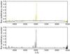 |
Fig. 2 Central spectrum for NGC 2273 (run2). Panels are the same as in Fig. 1. In this spectrum, the [Ne iii]λ3868 line can be clearly identified. |
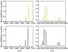 |
Fig. 3 Blue and red central spectra for NGC 3081 (run1). In the top panels, observed spectra (yellow lines) and templates (black lines) are shown. Bottom panels show the residuals of the fit. |
The emission-line fluxes were measured using the SPLOTtask in IRAF, by integrating the line intensity over a locally fitted continuum level. After marking two continuum points at both sides of the line, the flux was measured by taking into account the area, without any previous fitting of a Gaussian or any other assumed profile. Thus, asymmetries due to dynamical processes were indirectly considered. The corresponding uncertainties were estimated by adding in quadrature statistical errors measured by SPLOT, flatfielding errors, and the error in the flux calibration. Typical errors are of order ~ 5% (Table 2 shows the errors for the central apertures).
Emission line strengths for the central aperture.
The observed line ratios relative to Hβ are afterwards corrected for interstellar reddening, by determining the reddening coefficient c(Hβ) through the expression ![Mathematical equation: \begin{equation} {I(\lambda) \over {I({\rm H}\beta)}} = {F(\lambda) \over {F({\rm H}\beta)}} 10^{{\rm c}({\rm H}\beta)\left[f(\lambda)-f({\rm H}\beta)\right]}, \end{equation}](/articles/aa/full_html/2012/07/aa18292-11/aa18292-11-eq34.png) (1)where f(λ) is the Seaton (1979) reddening curve parametrized by Howarth (1984), and I(λ) and F(λ) are the intrinsic and observed emission line flux at wavelength λ, respectively. We employ the Balmer lines detected within our spectral ranges. As explained in Sect. 2, both arms of the run1 observations were treated separately to avoid the introduction of an additional continuum scaling error, hence the Hα/Hβ was unavailable. The extinction constant was then obtained from the average of the extinction constant obtained by fitting all available Balmer line ratios relative to Hβ, and the corresponding intrinsic or theoretical values. We considered the intrinsic flux ratio from Hummer & Storey (1987), assuming Te = 104 K and Ne = 100 cm-3. For these cases in which there is a high dispersion between the values for c(Hβ) obtained from different lines ratios, we used the extinction constant obtained from Hγ/Hβ alone. We assigned an internal extinction of zero to objects for which the observed Balmer decrement was lower than the theoretical values. The derived reddening was negligible for most of the spectra. In the case of NGC 4245, we obtained only Hβ and no other Balmer line, but did not consider this galaxy in the discussion. For NGC 1169, we observed only Hβ except at five galactocentric radii. For four galaxies, the observed Balmer decrement is lower than the theoretical one, so we consider as zero the internal extinction. In the fifth case, the obtained internal extinction is so low that the differences between the line fluxes, regardless of whether we consider this internal extinction, are lower than the obtained errors. Therefore, we assumed that there is negligible extinction in this galaxy.
(1)where f(λ) is the Seaton (1979) reddening curve parametrized by Howarth (1984), and I(λ) and F(λ) are the intrinsic and observed emission line flux at wavelength λ, respectively. We employ the Balmer lines detected within our spectral ranges. As explained in Sect. 2, both arms of the run1 observations were treated separately to avoid the introduction of an additional continuum scaling error, hence the Hα/Hβ was unavailable. The extinction constant was then obtained from the average of the extinction constant obtained by fitting all available Balmer line ratios relative to Hβ, and the corresponding intrinsic or theoretical values. We considered the intrinsic flux ratio from Hummer & Storey (1987), assuming Te = 104 K and Ne = 100 cm-3. For these cases in which there is a high dispersion between the values for c(Hβ) obtained from different lines ratios, we used the extinction constant obtained from Hγ/Hβ alone. We assigned an internal extinction of zero to objects for which the observed Balmer decrement was lower than the theoretical values. The derived reddening was negligible for most of the spectra. In the case of NGC 4245, we obtained only Hβ and no other Balmer line, but did not consider this galaxy in the discussion. For NGC 1169, we observed only Hβ except at five galactocentric radii. For four galaxies, the observed Balmer decrement is lower than the theoretical one, so we consider as zero the internal extinction. In the fifth case, the obtained internal extinction is so low that the differences between the line fluxes, regardless of whether we consider this internal extinction, are lower than the obtained errors. Therefore, we assumed that there is negligible extinction in this galaxy.
Emission line strengths for the central aperture are shown in Table 2. For NGC 4314, we show the emission line strengths for the innermost aperture (0.8 arcsec from the galaxy center) with detected emission. This central aperture corresponds to 0.75 arcsec for run1 galaxies and 0.4 arcsec for run2 galaxies. Values of [O ii], [Ne iii], and [O iii] are measured relative to Hβ = 100, and those of [N ii] and [S ii] to Hα = 100.
 |
Fig. 4 Diagnostic diagram for the emission-line regions of run1 galaxies at different galactocentric distances (R) scaled with R25. The solid line (Kewley et al. 2001) sets the star formation upper limit, the dashed line (Kauffmann et al. 2003) the empirical division between star-forming galaxies (SF) and transition objects (T), and the horizontal line (Kewley et al. 2006) separates Seyferts and Low-Ionization Nuclear Emission-line Regions (LINERs). |
For galaxies containing knots of gas emission, we also extracted spectra with apertures including all detected emission. In these cases, we corrected for extinction using an iterative method to determine, simultaneously, the underlying stellar absorption and interstellar reddening: we derived the extinction coefficient c(Hβ) for an assumed equivalent width of the stellar absorption EWabs that was the same for all observed Balmer lines. The assumed EWabs was varied until convergence between the c(Hβ) obtained from all the Balmer line ratios in use. The c(Hβ) values are in the range 0−2, and EWabs was found to be in the range 0.7−1.8.
4. Results
4.1. Star formation versus nuclear activity
Once the line fluxes had been measured and extinction-corrected, we compiled diagnostic diagrams commonly used to distinguish between star formation (SF) regions and regions containing or affected by an active galactic nucleus (AGN). However, classical diagnostic diagrams (log ([O iii]/Hβ) versus log ([N ii]/Hα) and log ([O iii]/Hβ) versus log ([S ii]/Hα)) (Baldwin et al. 1981; Veilleux & Osterbrock 1987) can only be applied to run1, owing to the limited spectral coverage of run2. For four galaxies, one from run1 and three from run2 we detected the [Ne iii]λ3868 line. This line has been proposed as an empirical indicator of metallicity (Nagao et al. 2006) as well as a diagnostic to distinguish between starburst galaxies and AGNs (see discussion in Pérez-Montero et al. 2007).
 |
Fig. 5 Diagnostic diagram for the emission-line regions of run1 galaxies for different galactocentric distances (R) scaled with R25. The solid line delineates our adopted separation between star formation regions and AGNs; below the dashed line there are LINERs and above it Seyferts (Kewley et al. 2006). |
 |
Fig. 6 Diagnostic diagram for those galaxies in which we have detected the [Ne iii]λ3869 line. The solid line indicates the limit between star-formation regions and AGNs, and the dashed one between LINERs ([O iii]5007/Hβ ≤ 0.5) and Seyferts 2 ([O iii]5007/Hβ > 0.5) (Rola et al. 1997). |
Figures 4 − 6 present the diagnostic diagrams, in the first two figures at different galactocentric distances. In Fig. 4, we have plotted the theoretical curves of Kewley et al. (2001), which sets the maximum expected [O iii]/Hβ at a given [N ii]/Hα for a star-forming region, the curves of Kauffmann et al. (2003) that empirically divides star-forming galaxies from transition objects, and that of Kewley et al. (2006) separating Seyfert from low-ionization nuclear emission-line region (LINER) galaxies. In Fig. 5, we plot the relation between the line ratios log ([S ii]/Hα) and log ([O iii]/Hβ) for the galaxies in our sample at different radii. The theoretical models separating the values corresponding to ionization by star formation and AGN are also indicated. Rola et al. (1997) proposed an alternative diagnostic diagram based on the [Ne iii]λ3869 line. In Fig. 6, this diagnostic diagram for galaxies in which we have detected this line is plotted, relating log ([Ne iii]/Hβ) with log ([O iii]/Hβ). The solid line indicates the limit between star-formation regions and AGNs, and the dashed one between LINERs ([O iii]5007/Hβ ≤ 0.5) and Seyferts 2 ([O iii]5007/Hβ > 0.5) as explained in Rola et al. (1997).
 |
Fig. 7 Radial distribution of log ([O iii]/Hβ) (for active galaxies of run1) and log ([Ne iii]/Hβ) (for run2 galaxies with [Ne iii]λ3869 line detected). The theoretical curves of Kewley et al. (2001, for log ([O iii]/Hβ) and log ([N ii]/Hα)) and Rola et al. (1997, for log ([Ne iii]/Hβ)) distinguishing between AGN and SF are also plotted with dashed and solid lines, respectively. |
Figures 4 and 5 also show that at large radii, there is a higher probability that the gas is ionized by star-forming regions, while central emission is characterized by AGN-like line ratios.
Studying the diagnostic diagrams for individual galaxies, we confirm the classification carried out by Veron-Cetty & Veron (2006) with the exception of NGC 5101 and NGC 1433. According to the emission line in the central region, we reclassify NGC 5101 as a LINER even though it was not classified in this way in Veron-Cetty & Veron (2006). Our classification agrees with Moiseev (2001). The run1 galaxies that were not classified as Seyfert or LINER, NGC 2665, and NGC 2935, are transition objects. In Table 1, we compare the nuclear type obtained in this paper with that from a previous classification carried out by Veron-Cetty & Veron (2006).
Since we have radial information for the diagnostic diagrams, we considered the question of the AGN influence region by analyzing the radial behavior of the diagnostic ratios, to find the radius at which star formation starts being the main photoionisation source. Figure 7 shows the radial distribution of log ([O iii]/Hβ) (or log ([Ne iii]/Hβ)). In the same figure, we have plotted the measured values of [N ii]/Hα. With these values and taking into account the theoretical curve of Kewley et al. (2001) (or Rola et al. 1997 for log ([Ne iii]/Hβ)), we obtained the limiting for either star formation or nuclear activity, which are indicated by a dashed line. At a given galactocentric radius, if the observational points are above these lines, a star-forming region is not the main photoionization component at that radius. The AGN or LINER is the dominant ionization mechanism up to different radii for different galaxies: for example, for NGC 2273 evidence of the ionization by an AGN is present only at the smallest considered radii. For NGC 2217, the influence region of AGN extends to ~0.1 kpc.
4.2. Oxygen abundances and gradients
The measurement of nebular gas abundances has several difficulties. The direct method to calculate oxygen abundances involves the use of the ratios of temperature sensitive lines, such as [O iii]λλ4959, 5007/λ4363 (Osterbrock 1989). Unfortunately, when the metallicity increases, the electronic temperature decreases and the auroral lines (e.g. [O iii]λ4363) become too weak to be measured in most extragalactic objects, hence we have to find empirical, semiempirical, and theoretical calibrations to calculate abundances. Some relations between the gas metallicity and line flux ratios of strong emission lines have been found. A drawback of these indicators is that they have been basically developed for low-metallicity H ii regions, where the [O iii]λ4363 line is easily observed. However, it has been made considerable efforts to study high metallicity H ii regions (e.g. Castellanos et al. 2002; Bresolin 2007), since these are the most abundant in early-type spiral galaxies and the central regions of late-type spiral galaxies (Vila-Costas & Edmunds 1992). Although semiempirical methods provide better results in statistical studies than individual values (Pérez-Montero et al. 2007), we used these methods to estimate the oxygen abundance variations with galactocentric radius. Systematic discrepancies among different methods have been found (see, for instance, Kewley & Ellison 2008; López-Sánchez & Esteban 2010, and references therein), so we used several methods to study the dependence of the results on the method chosen.
An additional problem is that 11 out of our 20 galaxies have been classified as either LINERs or Seyferts. The mechanism of ionization in the case of LINERs is still not well-understood, so there are no methods for estimating abundances in the central parts of these galaxies. Some methods exist in the case of Seyferts, but owing to our limited spectral coverage we can only apply one of them, and in some particular cases. We also apply this method in LINERs, powered by some process which may be in-between AGN excitation and photoionization due to star formation.
4.2.1. Nebular abundances: errors in their determination and comparison between different methods
We use different methods to estimate the nebular abundances for the two different runs, as the spectral range covered in both data sets is different. The brightest lines measured, apart from the Balmer (Hγ, Hβ, Hα) lines are the [O iii]λλ4959, 5007, [N ii]λλ6548, 6583, and [S ii]λλ6717, 6731 lines for run1 galaxies, and [O ii]λ3727 and [O iii]λλ4959, 5007 for run2 galaxies. At some distances from the center, [O iii]λ4959 is not detected, in which case we assume that [O iii]λλ4959, 5007 = 1.337[O iii]λ5007 (Oey & Kennicutt 1993).
 |
Fig. 8 Relation between different calibrations for obtaining oxygen abundances. In panels a) − d), we compare the methods used for run2 galaxies with the R23 calibration by McGaugh (M91). In panels e) and f), the comparison is for run1 galaxies, between N2 and either O3N2 or SB1. The solid line in each plot shows the agreement between the different methods. |
The abundance indicators used in this work are:
-
1.
R23: on the basis of this parameter(R23 = ( [OII] λ3727 + [OIII] λλ4959,5007] )/Hβ), we use two calibrations:
-
M91: the theoretical calibration of McGaugh (1991), which takes into account the influence of the ionization parameter to determine the chemical abundance.
-
Z94: it is an analytical calibration derived by Zaritsky et al. (1994) from the average of three previous R23 calibrations (Dopita & Evans 1986; McCall et al. 1985; Edmunds & Pagel 1984). It is only valid for high metallicity objects with log (O/H) + 12 > 8.35.
-
-
2.
N2: this uses
![Mathematical equation: \hbox{$\left({[\rm NII]\lambda 6583} \over {\rm H\alpha}\right)$}](/articles/aa/full_html/2012/07/aa18292-11/aa18292-11-eq54.png) (Pettini & Pagel 2004), which has the advantage of not being double-valued with oxygen abundance, and that lines are very near each other, minimizing the dependence on the reddening correction.
(Pettini & Pagel 2004), which has the advantage of not being double-valued with oxygen abundance, and that lines are very near each other, minimizing the dependence on the reddening correction. -
3.
O3N2: this depends on
![Mathematical equation: \hbox{$\left({[\rm OIII]\lambda 5007/\rm H\beta} \over {[\rm NII]\lambda 6583/\rm H\alpha}\right)$}](/articles/aa/full_html/2012/07/aa18292-11/aa18292-11-eq55.png) (Pettini & Pagel 2004) and is a monotonic function of the oxygen abundance. However, in our present study, the pairs of lines ([O iii]λ5007, Hβ) and ([N ii]λ6583, Hα) are detected in separate spectra, which can introduce errors caused by a mismatch between the continuum fluxes in the red and blue (run1) ranges. This problem is discussed at the end of this section.
(Pettini & Pagel 2004) and is a monotonic function of the oxygen abundance. However, in our present study, the pairs of lines ([O iii]λ5007, Hβ) and ([N ii]λ6583, Hα) are detected in separate spectra, which can introduce errors caused by a mismatch between the continuum fluxes in the red and blue (run1) ranges. This problem is discussed at the end of this section. -
4.
O2Ne3: Pérez-Montero et al. (2007) discussed the relation between [Ne iii]λ3869 and [O ii], and defined the parameter
![Mathematical equation: \hbox{$O2Ne3={{I([{\rm OII}]\lambda 3727)+15.371([{\rm NeIII}]\lambda 3869)} \over {I({\rm H\beta})}}$}](/articles/aa/full_html/2012/07/aa18292-11/aa18292-11-eq56.png) . Taking into account this parameter, we calculated the oxygen abundance with the expression of M91. This line is more intense in AGNs because, in these objects, Ne+2 is less suppressed than in star-formation regions, as explained in Rola et al. (1997).
. Taking into account this parameter, we calculated the oxygen abundance with the expression of M91. This line is more intense in AGNs because, in these objects, Ne+2 is less suppressed than in star-formation regions, as explained in Rola et al. (1997). -
5.
SB1: this was calibrated for active galaxies (Storchi-Bergmann et al. 1998) and has two different calibrations. It is valid for Seyfert galaxies but not so accurate for LINERs. We used the calibration involving the [O iii], [N ii], Hα and Hβ lines because of our observed spectral range, which depends on the gas density, and is valid only for 100 < N < 10 000 (where N is the gas density in cm-3) and 8.4 < 12 + log (O/H) < 9.4.
-
6.
KD02: this method was proposed by Kewley & Dopita (2002), which consists of an iterative scheme involving the ionization parameter and R23.
-
7.
P05: Pilyugin & Thuan (2005) improved the calibration of Pilyugin (2000, 2001) with a more extended (in metallicity) set of H ii regions. The lines needed to measure this indicator are [O ii]λλ 3727, 3729, [O iii]λλ 4959, 5007, and Hβ.
We applied R23, O2Ne3, KD03, and P05 methods to galaxies observed in run2 and N2, O3N2, and SB1 to those observed in run1.
Several of the indices described above have two branches in their calibration, i.e., there are two possible metallicity values for a given index. This makes it necessary to have additional criteria to distinguish between the upper and the lower branches. We adopt the high-metallicity values based on (a) the empirical diagrams of Nagao et al. (2006) (though not for active galaxies). With a sample of 50 000 spectra, they proposed a method based in the monotonic metallicity dependence of [O iii]λ5007/[O ii]λ3727, that enabled the R23 degeneracy to be broken. We made use of their diagrams to determine the branch. (b) The Kobulnicky et al. (1999) conclusion about galaxies in the local Universe (i.e. objects more luminous than MB ~ −18 have metallicities higher than 8.3, and the whole sample lies within this range). (c) Galaxy morphologies, all the galaxies being of early-type and Oey & Kennicutt (1993) found that the average metallicity value for H ii regions in Sa and Sb galaxies is 8.97, clearly in the upper region. (d) In NGC 1530, this these high-metallicity values are similar to those found by Márquez et al. (2002) using the [N ii]/Hα ratio. A special case is that of NGC 1358: the R23 values calculated for this galaxy are in the limit of applicability of the methods based on this parameter. However, using data for [N ii] and Hα we calculated abundance values consistent with these obtained using the R23 method.
The errors in the oxygen abundances were estimated by means of the error propagation of the uncertainties in the relevant line fluxes and range between ~0.01 and 0.10 dex (or 10 − 20% in [O/H]). This is smaller than the intrinsic scatter associated with the empirical calibrations of the so-called strong-line methods (e.g. 0.2 dex for R23, Athey & Bregman 2009). We carried out various tests to determine the uncertainties introduced into the different parts of the analysis. Abundances were estimated in two possible ways for each test of this analysis. In what follows, we describe the maximum differences found and the mean values of these differences in a galaxy chosen as a characteristic example:
-
(a)
As discussed in Sect. 3, in most of the spectra weused stellar templates to subtract the contribution from theunderlying stellar population, an approach that provides a secondway to correct the line intensities with an iterative method. Thedifferences found in the gaseous abundances between bothmethods are smaller than 0.1−0.2 dex. As an example, for NGC 1433 the mean values of these differences are 0.04 ± 0.06 dex for N2, 0.05 ± 0.03 dex for O3N2, and 0.04 ± 0.02 dex for SB1.
-
(b)
Considering either an equivalent width due to Balmer absorption of 2 Å to correct the stellar absorption, a typical value used in the literature (e.g. Zaritsky et al. 1994), or using the iterative method to estimate it, introduces differences smaller than 0.1−0.2 dex. For example, in NGC 1530 the mean values of these differences are 0.04 ± 0.04 dex (R23), 0.05 ± 0.04 dex (Z94), 0.03 ± 0.02 dex (KD03), and 0.13 ± 0.09 dex (P05).
-
(c)
The error introduced if we were to consider an I(Hα)/I(Hβ) value of either 2.85 or 3.1 is as small as 0.05 dex. Annibali et al. (2010) also showed that, in any case, considering Hα/Hβ = 2.85 does not significantly change the results. For NGC 3081, mean differences are 0.0004 ± 0.0008 dex (N2), 0.003 ± 0.004 dex (O3N2), and 0.08 ± 0.09 dex (SB1).
We next show that differences among the different metallicity calibrations are larger than these errors.
We compare the results from the different methods in Fig. 8, taking N2 as a reference for run1 galaxies, and R23 (M91) for run2 galaxies. The values of O2Ne3 could only be calculated for three galaxies; its behavior is the same as the R23 (M91) but has a larger dispersion. The measurement for R23 (Z94) is valid for 12 + log (O/H) > 8.35 (Zaritsky et al. 1994). For 12 + log (O/H) values between 8.35 and 8.7, the R23 method, with the calibrations of Z94 and M91, provide similar metallicity values, but from 8.7 upwards, the Z94 value becomes higher than the M91 one. In KD03, the behavior is the same as in R23 (M91), but KD03 gives values slightly above those of R23 (M91) from 8.2 upwards. The P05 values are systematically 0.3 − 0.5 dex lower than those of R23 (M91) with the exception of NGC 1358. Bresolin et al. (2009) showed that, for the external parts of the disk of M83, the variation in metallicity with [N ii]/[O ii] is closer to the actual values, being 0.4 dex lower than those obtained with R23. Therefore, the metallicities derived using the P05 method might be expected to be more realistic or, at least, closer to the direct metallicity determinations. Kennicutt et al. (2003) found systematic differences of up to 0.5 dex between the Te and R23 abundances. Pilyugin & Thuan (2005) noted that the determination of oxygen abundances using P05 agrees with the Te abundance to within 0.1 dex, even at high metallicity, as in our case.
For run1 galaxies, the largest differences between O3N2 and the N2 index are 0.3 − 0.4 dex, except for NGC 3081, for which the difference is around 0.5 dex. Denicoló et al. (2002) emphasized the importance of the N2 method, showing that the O3N2 calibration did not improve the results. We note that SB1 is a method calibrated for AGN; though 11 of the galaxies studied here have been classified as active, this method has only been used in the cases that meet the above conditions of density and metallicity, and only to run1 galaxies because of the lines involved.
It is interesting to compare the radial dependence of the values obtained with the different methods, to study either the effect of nuclear activity or the differences due to the physical differences between the nuclear and disk H ii region properties. The H ii characteristics can influence the abundance trends obtained using different methods in different ways (Kennicutt et al. 1989). The systematic differences are presented later in our comparison with stellar metallicities. Figure 9 shows the residual values of the different abundance-calculation methods for all the galaxies with respect to R23 (M91) for run2 galaxies and N2 for run1 galaxies.
 |
Fig. 9 Differences between the oxygen abundances obtained with the different methods versus the galactocentric radius for each galaxy. R25 has been taken from HyperLeda. Residuals are with respect to R23 (M91) for run2 galaxies and to N2 for run1 galaxies. Crosses are oxygen abundances obtained from the O2Ne3 calibration, triangles from R23 (Z94), circles from KD03, squares from P05, diamonds from O3N2, and asterisks from SB1. |
 |
Fig. 10 Oxygen abundances of 12 + log (O/H) obtained with O3N2 for run1, and with R23 (M91) for run2, versus R/R25 in each galaxy. Dashed lines indicate the fits to all measured values, and solid lines show the best fits within the bulge region. For run1 galaxies, black lines indicate the N2 fit, cyan lines the O3N2 fit, and blue line the SB1 fit. For run2 galaxies, black lines show the R23 (M91) fit, blue lines the Z94 fit, green lines the KD03 fit, and red lines the P05 fit. |
 |
Fig. 10 continued. |
Central abundances, for run2 galaxies.
As already noted, our P05 abundances are always below R23 (M91), the difference being around 0.5 dex, without any variation with radius (with the exception of the special case NGC 1358 as we have mentioned). For KD03, the largest differences are found in the central part of the Seyfert galaxy NGC 1358, which are much smaller outside radii of 0.08 R/R25, indicated as the activity zone in Fig. 7. However, this is not the result typically found for Seyferts (see NGC 2273), for which we personally find similar values to those calculated with R23 calibrations by M91 and Z94. We find a larger dispersion for O2Ne3 than for the other methods, without any systematic trend with radius, the largest deviation occurring for galaxies that have fewer radial bins (e.g. NGC 4314). Between O3N2 and N2, the differences are small in most galaxies, less than 0.2−0.3 dex. However, for two galaxies, NGC 3081 and NGC 2217, these differences are larger (0.4−0.5 dex), but then become smaller (again 0.1−0.2 dex) with radius, at larger galactocentric distances.
As above mentioned, 11 galaxies have been classified as Seyferts or LINERs. All methods used here to derive metallicity, with the exception of SB1, have been derived for star-forming galaxies. We can only use the specific calibration method SB1 in 3 of our 20 galaxies, NGC 1433, NGC 2217, and NGC 3081, even though only one of these, i.e. NGC 3081, is clearly a Sy2. Annibali et al. (2010) compared oxygen abundances estimated from a photoionization model based on R23 (Kobulnicky et al. 1999) with SB1. The values obtained from the SB1 method are on average ~0.04 dex higher than those for the R23 calibration, but the differences between both metallicity values in individual regions can be as large as 0.3 dex. Keeping this result in mind, we have opted to show the values obtained with all the methods for comparison. This can be specially useful in the case of LINERs, whose mechanism of ionization is unknown. Therefore, we have calculated the abundance values with SB1 whenever possible. For the active galaxies for which this method cannot be used, we only indicate the metallicities obtained from methods calibrated for star-forming regions, and we caution the reader again about the validity of these values for AGN-dominated regions.
4.2.2. Gas oxygen-abundance in barred galaxies
Figure 10 shows the oxygen abundances obtained with R23 (M91) or O3N2 versus radii for all galaxies. We have linear fits performed in the bar region and in the bulge region taking into account the errors derived from the line fluxes.
Tables 3 and 5 show, respectively, for run2 and run1, the value of oxygen abundances within an aperture of 1.2 arcsec (i.e. after averaging abundances within the central 1.2 arcsec), the central abundance inferred by extrapolating to R = 0 the linear fit (for only R23 (M91) and O3N2), and the central value from the extrapolation to R = 0 excluding the region of influence of the AGN. Tables 4 and 5 show gradients for all used methods (in units of dex/arcsec), taking into account all the nebular emission in the bar region and their errors. Galaxies classified as either Seyferts or LINERs are marked with a dagger. For the galaxies for which we have enough points, we have two rows in these tables: the first one shows values obtained in the bar region, and the second those obtained excluding the AGN-affected region determined in the previous section. These regions affected by an AGN have been determined from Fig. 7, except for NGC 2681, NGC 2859, and NGC 4394 for which we have considered the radial ranges reported by Véron-Cetty & Véron (2006) and references therein. The numerical values are shown in Tables 3 and 5.
The seeing size could introduce errors in our measurements of the gradients. To study this effect, we produced artificial spectra at each pixel position, which we then convolved with Gaussians of different widths, covering the seeing values of these observations. This procedure was performed using the IRAF GAUSS task. We then generated three spectra. The largest differences in abundances calculated for these three spectra are smaller than 0.2, implying that the differences in the gradients are of ~5%.
We analyzed our results using the indices R23 (M91) and O3N2. For run2 galaxies, differences are nearly constant at all radii, in such a way that gradients maintain their sign in nearly all methods. In run1 galaxies, there are variations with galactocentric distance as mentioned above. In particular, the three galaxies for which we applied the SB1 method are also the galaxies with the largest differences in abundances in the central region, which are lower for O3N2 than for N2. This difference does not persist to larger radii, so the gradient sign is opposite for the two methods. The oxygen abundances in a 1.2 arcsec aperture are in the range 8.4−9.1 dex.
If we consider all the detected emission in the bar region at a 3-σ significance, for the star-formation galaxies, we detect a positive gradient for three galaxies (NGC 1169, NGC 2523, and NGC 2935) and a negative gradient for two galaxies (NGC 1832 and NGC 2962). For LINERs, we find a positive gradient for three galaxies (NGC 1433, NGC 4314, and NGC 4394) and none of them have a negative gradient. We find that for the region unaffected by any AGN that may be present in these galaxies, the sign of the gradients does not vary. In the case of Seyferts, we find negative gradients in four galaxies when we consider the bar region, but when we exclude the AGN-affected region, three of them keep their gradient sign. Only one of the Seyfert galaxies has a positive gradient, which is unaffected by the AGN region.
In most disks of spiral galaxies, both barred or unbarred, negative metallicity gradients have been obtained (e.g. Bresolin et al. 2009; Garnett & Shields 1987, etc.). This gradient seems to be shallower for barred than unbarred galaxies, and higher for late-type than for early-type galaxies (Hidalgo-Gámez et al. 2011; Vila-Costas & Edmunds 1992; Zaritsky et al. 1994). All our galaxies are barred and early-type; hence, based on previous studies, the gradient should be shallow. We find gradients in the range [− 3.7, 1.4] (normalized to R25) with the exception of NGC 1169, which has a very large dispersion in its abundance values. In Sect. 5, we compare these values with those found in the literature.
In Tables 6 and 7, we present the obtained gradients for the bulge region for all adopted methods, and the central oxygen abundance (only with R23 (M91) or O3N2 method). In these tables, we have marked the active galaxies but the gradients are fitted including the AGN regions. NGC 3081 is the only Seyfert galaxy for which we have been able to calculate abundances with the SB1 method. For two galaxies (NGC 1169 and NGC 5101), all the measured nebular emission in the bar position is in the bulge zone where the scatter is larger than in the bar region and, therefore, errors are also larger. We find the same sign for the slopes in most of the star-forming galaxies. They are in general steeper than those measured when the bar region is considered.
Oxygen abundance gradients for all adopted methods and the central abundance, for run2 galaxies.
4.3. Comparison of the nebular gas abundances with the distribution of stellar metallicities
While measurements of the ionised gas abundances give information about the current composition of the ISM, the stellar metallicities are directly linked to the star formation history and, thus, a comparison between the metal abundances of both components can help us to determine the origin of the gas involved in the present star formation.
In previous works (Pérez et al. 2007, 2009; Pérez & Sánchez-Blázquez 2011), we derived the radial distribution of the stellar ages and metallicities along the bar and the bulges of the galaxies presented in this work. Line strength indices were measured and used to derive age and metallicity gradients in the bulge and bar region by comparing with stellar population models.
Figure 11 shows the comparison of the stellar and ionized gas abundances along the radius for all the galaxies. For the sake of clarity, the radius is on a logarithmic scale and R = 0 is shifted to log (R) = −0.5. For run2 galaxies, the R23 (M91) calibration has been chosen, covering the error bars the values obtained with all methods with the exception of O2Ne3. The values obtained with all methods have been represented in the case of run1 galaxies. For the comparison, we have assumed as reference the solar value 12 + log (O/H)⊙ = 8.69 (Allende-Prieto et al. 2001) and [Fe/H] for both components. We have indicated by a vertical line the influence region of any active nuclei. In this way, we again caution (Sect. 4.2.1) the reader that may be incorrect to compare the gas abundances with the stellar metallicities in the regions dominated by an AGN.
Oxygen abundance gradients derived using all adopted methods, for run1 galaxies.
Metallicity gradients in the bulge regions with all the adopted methods for run2 galaxies, including AGN-affected regions.
Metallicity gradients in the bulge regions, with all the used methods, for run1 galaxies, including AGN regions.
For the following run2 galaxies, the nebular metallicities lie clearly below the stellar metallicity values: NGC 1169, NGC 2962 (in agreement with Marino et al. 2011), and NGC 4394. Only NGC 4394 is classified as a LINER. This lower metallicity gas (w.r.t. the stellar metallicity) is located in the bulge region, and similar values for the metallicity of both components are found elsewhere. For run1 galaxies, nebular metallicities obtained with O3N2 are lower than stellar metallicities in NGC 2217, NGC 3081, and NGC 4643. However, with the values obtained with N2, they are very similar (NGC 3081 and NGC 4643) or even higher (NGC 2217). These three galaxies are classified as AGNs. If we consider SB1, a nebular metallicity is of the same order as the stellar metallicity for NGC 3081 (Sy) and NGC 2217 (LINER).
For some of the other galaxies, the distribution of the gas and the stellar abundances closely follow each other and for 3 galaxies the gas abundances lie clearly ( ≥ 0.2 dex) above the stellar metallicities.
Not many works have addressed a direct comparison between the metallicities obtained from the stars and the ionized gas. Storchi-Bergmann et al. (1994) concluded that both abundance measurements are well-correlated for star-forming galaxies. However, recent work (Marino et al. 2011) suggests, as derived from HI and GALEX UV imaging, the presence of current star formation activity in early-type galaxies with emission lines. This sort of galaxy rejuvenation could be due to external gas re-fueling. This accretion would indicate that there are differences between the metallicities of the old stellar component and the newly accreted gas responsible for the present star formation. Furthermore, Annibali et al. (2010) found in a comparison between nebular and stellar metallicities of E-S0 galaxies with nebular emission that the gas metallicity tends to be lower that the stellar metallicity, the effect largest being for the highest stellar metallicities.
In Figs. 12 and 13, we compare the gradients obtained for the oxygen abundances along bars and the bulge regions with those estimated in Paper II. They are normalized to R25 ((12 + log (O/H))/(R/R25)) values. In Paper I, we found that the stellar metallicity gradients along the bar show a large variety. The distribution of the gas nebular abundances in the bar region have a mild gradient (flatter than for the stellar component for star-forming galaxies except for NGC 1169), and we do not see any clear relation between the stellar and nebular gas metallicity gradients. With respect to the bulge region, gradients for the stellar component in star-forming galaxies are flatter than the gaseous gradients for NGC 1169 and NGC 2523. In the studiable cases, the oxygen abundance gradients are, in general, steeper for bulges than bars, and have the same sign. However, this is not the case for the stellar abundance gradient, where the sign between the bulge and the bar gradient changes in 10 out of 16 galaxies.
 |
Fig. 12 Comparison of the metallicity gradients obtained for the gaseous and stellar components in the bar region of our sample galaxies. They are normalized to R25 (i.e. the gradients have been obtained from linear fits to the 12 + log (O/H) versus R/R25 representation for each galaxy). Circles are those estimated with the R23 (M91) or N2 methods, squares are the mean value of gradients calculated with all methods (the error bar covers the range of these gradients), and stars are the gradient [Z/H] for the stellar component (Paper II). Order indicated along the abscissas is that of Tables 6 and 7. Filled symbols represent star-forming galaxies. |
 |
Fig. 13 Comparation between metallicity gradients obtained for gaseous and stellar components in the bulge region of our sample galaxies. They are normalized to R25 (i.e. the gradients have been obtained from linear fits to the 12 + log (O/H) versus R/R25 representation for each galaxy). Circles are those estimated with the R23 (M91) or N2 methods, squares are the mean value of gradients calculated with all methods (the error bar covers the range of these gradients), and stars are the gradient [Z/H] for the stellar component (Paper II). The order along the abscissas is that of Tables 6 and 7. Filled symbols represent star-forming galaxies. |
5. Discussion
We have found that most of the emission is centrally concentrated in the bulge region. This had been noted in previous studies and seems to be independent of the presence of a bar (Davis et al. 2011). In 5 galaxies, emission lines are present along the whole extension of the bar, and 6 out of the 18 galaxies have some star formation at the bar ends as well as in the bulge region. Previous works have claimed that the distribution of star formation in a bar is correlated with the bar age; younger bars ( < 1 Gyr) host star formation along the entire bar, while older bars have star formation at the bar-ends and nuclear regions (Phillips 1993; Martin & Friedli 1997; Martin & Roy 1995; Friedli & Benz 1995; Verley et al. 2007). However, some of the galaxies for which nebular gas is found along the bar seem to host bars that are old (see Paper I). Therefore, the star formation distribution in these bars is possibly more related to the reservoirs of gas that could replenish the bar than to the actual time of bar formation.
We have found neither a relation between the difference in abundance values between different methods and the type of the galaxy, nor any relation to the galactocentric distance in which the lines are measured (see Sects. 4.2.1 and 4.2.2).
We have considered the possible systematic effect of an AGN nuclei on the determination of abundances. Its effect is difficult to quantify, but very important when comparing with the stellar metallicities in the inner regions of these galaxies and deriving the abundance gradients. The central regions consist of a mixture of different components with different physical properties (Lindblad & Fathi 2011) and introduce difficulties in determining the main ionising mechanisms. Most of the central abundances derived in the works mentioned above, have not considered the influence of an active nuclei. Their abundance estimations have been carried out in H ii regions or/and in star-forming galaxies, so the models for calibration are based on stellar photoionization alone. Storchi-Bergmann et al. (1998) proposed two calibrations for active galaxies: the first one depending on [N ii]/Hα and [O iii]/Hβ (SB1), and the second, a linear combination of log [N ii]/Hα and [O ii]/[O iii] (SB2). They concluded that, when possible, the best option is to use the mean value of both. Based on the extrapolation of metallicities towards the nuclear regions, they found that this calibration is good for Seyferts, but that there is no clear conclusion for LINERs. We have used this method, SB1, for only three galaxies of run1. We have been unable to estimate SB2 for them because we could not measure [O ii]. For these galaxies, 2 LINERs and a Sy, we have compared abundances calculated with SB1 and N2 and O3N2, which would be the extreme cases i.e. of either AGN or photoionization produced by hot stars. For LINERs, the results of SB1 match or are closer to those of O3N2 in the central regions, while for the Seyfert galaxy they are similar to those estimated with N2. In any case, the difference between oxygen abundances derived using N2 or SB1 is less than 0.2 dex, a value considered as the intrinsic uncertainty in the models used to calibrate R23. Although the presence of an AGN does not seem to alter the results, we caution that the results for these regions may be influenced by AGNs.
We then compared the oxygen abundances with the stellar metallicities. We found that the central metallicities, 12 + log (O/H), have a mean value within 1.2 arcsec in the range from 8.4 to 9.1. These values agreed with those found in the inner parts of early-type spirals. Oey & Kennicutt (1993) studied H ii regions in 15 Sa to Sb galaxies, obtaining abundance values, derived using the R23 method, from 8.7 to 9.2. The larger values correspond to regions located at smaller galactocentric radii. They found that gas metallicities in these galaxies are systematically higher than those in Sc and later-type galaxies. Zaritsky et al. (1994) suggested that this relation might be indicative of a dependence on galaxy mass and not with galaxy type after analyzing H ii regions in a sample of 39 galaxies covering morphological types from Sab to Sd. They found metallicities in the range 8.2 − 8.6, similar to the abundances of our work, although we cover morphological types from SB0 to SBbc. Vila-Costas & Edmunds (1992) also found a correlation between the central gas abundances and galaxy masses, by analyzing the gas metallicity distribution of 32 disk galaxies of different morphological types. For the centers of Sab-Sb galaxies they found oxygen abundances in the range 8.7 − 9.5. A large statistical study using SDSS data by Tremonti et al. (2004) analyzed 53 000 star-forming galaxies at z ~ 0.1. In this study, the authors addressed the fundamental role that the galaxy mass plays in its chemical evolution. They found a strong correlation between mass and nebular oxygen abundance for galaxies with masses between 108.5 and 1010.5 M⊙, with a flattening of the relation for higher galaxy masses. Some recent studies investigating how mergers and bars can modify this correlation (Ellison et al. 2011) have measured a higher nebular abundance in barred than unbarred galaxies of the same mass. Our galaxies lie on the flat part of the correlation, hence we do not expect to find any strong correlation between the rotational velocity and the nebular abundance.
However, we see in Fig. 14 that the galaxies with the lowest abundances are those with the highest rotational velocities, although there is a large dispersion in the values, since we also find galaxies with high rotational velocity and high ionized gas metallicities. However, there are no galaxies with low (12 + log (O/H) < 8.68) nebular abundances and low rotational velocities. The only exception is NGC 3081 (Seyfert) for the oxygen abundance obtained using O3N2. This result might indicate that we cannot exclude the idea that some rejuvenation mechanism operates in some of the most massive galaxies in our sample.
 |
Fig. 14 Rotational velocity corrected for inclination versus central oxygen abundances (1.2 arcsec). Filled circles represent those calculated using the R23 method for run2 and O3N2 for run1. Squares are values obtained with N2 for run1. |
Following this result for the trend in nebular abundances with disk rotational velocities, we search for nebular abundance trends with stellar velocity dispersion, but we find no such trend. As for the stellar abundances, we find in Paper II, as expected from other studies, a correlation between stellar central abundances and central velocity dispersion (see Fig. 15).
 |
Fig. 15 Stellar velocity dispersion versus central oxygen abundances (1.2 arcsec). Filled circles represent those calculated using the R23 method for run2 and O3N2 for run1. Squares are values obtained with N2 for run1. |
When comparing these central nebular abundances with central stellar metallicities, we find that for three galaxies the nebular abundances are significantly lower than the stellar metallicities. The galaxies which show nebular abundances lower than the stellar metallicities are systematically among the galaxies with the highest rotational velocities in our sample.
The bar is thought to provide an efficient mechanism for quickly redistributing material within the disk. External accretion via the bar potential is a plausible mechanism for bringing new gas to the center and diluting the central gas metallicities. The strength of the bar determines the gas inflow rate (e.g. Athanassoula 1992, 2000), although no clear trend between the bar strength and nebular composition is found for our galaxies. The efficiency of this process might be limited by the availability of gas, and despite no clear trend with HI mass being found we note that we lack information about the total gas content of our galaxies. Other processes capable of explaining the existence of low metallicity gas at the center of these massive galaxies include cold flows to the center (Kereš et al. 2005) and particular star-formation histories (Yates et al. 2012). Yates et al. (2012) conclude, by examining semi-analytical models, that massive galaxies with low nebular abundances have undergone a gas-rich merger with a later shut-down of star formation. This low density metal-poor gas accretion is insufficient to form stars efficiently and subsequently dilutes the gas-phase metallicities. Further information of the total gas content and both its distribution and kinematics would help us to elucidate the different external accretion mechanisms that might operate in these galaxies.
As for the nebular abundance gradients found in this work, numerical models of barred galaxies (Friedli et al. 1994) show that the initial slope of the abundance is only slightly modified in the bar region, while outside the bar corotation radius, the original slope gets flatter. We estimated the gas oxygen abundances along the bars to study the efficiency of mixing by the bar within the corotation radius. Considering only star-forming galaxies, we find positive gradients, with a 3-σ significance, for the oxygen abundance in the bar regions of three galaxies and negative gradients in two other galaxies. The estimated gradient values range from − 3.7 to 1.4, in units of dex/(R/R25) with the aforementioned exception of NGC 1169. In eight of the observed galaxies, the gradient is shallower than 0.5 dex/(R/R25). In the bulge region, where most of the emission is found, we find steeper gradients.
It is, however, not a simple task to interpret the origin of these gradients because it is not only stellar evolution, star formation, and bar dynamics, all complicated processes, that affect the gradients but the refueling of newly accreted gas could also change the gradient. Naively, central accretion of gas would dilute the inner regions generating a positive gradient, while the effects of radially accreted gas may not be sufficiently evident without proper modeling. However, it would be possibly to reduce a pre-existing gradient because of the rapid mixing and reactivation of star formation in the bar region (Friedli et al. 1994; Friedli & Benz 1995).
Most gas metallicity gradients that can be found in the literature include the whole disk; van Zee et al. (1998) found gradients in the range [−0.30, −1.52] dex/R25 for spiral galaxies, and Rupke et al. (2010) a mean value of − 0.57 ± 0.05 considering 11 isolated spirals. Oey & Kennicutt (1993) concluded that barred galaxies have a shallower gradient than unbarred ones. However, a large range of abundance gradients have been found, some of them being much steeper than for unbarred spirals (Edmunds & Roy 1993; Considere et al. 2000). Vila-Costas & Edmunds found gradients ranging from − 3.33 to − 0.899 for non-barred galaxies, and from −0.156 to −0.398 for barred galaxies (all in dex/R25). Zaritsky et al. (1994) obtained a mean value of −0.23 dex/R25 for five barred galaxies. In particular, for the Milky Way, Balser et al. (2011) measured a radial gradient of − 0.0446 ± 0.0049 dex/kpc. Edvardsson (2002) found a value of − 0.07 ± 0.01 dex/kpc for galactocentric distances of between 6 and 18 kpc.
The discrepancy between the values found in the literature for the disk and our values, concerning only the bar region, could be due to the predicted change in the slope around the bar radius (Friedli et al. 1994). Furthermore, we have found a slope change between the bulge and the bar region, which was also predicted by Friedli et al. (1994). These changes in the abundance slope with radius, such that the gradient is steeper in the inner parts of the galaxies, have been analyzed by various authors. Zaritsky et al. (1994) found that the gradient in the bar of NGC 3319 was different from that outside it. This question was studied by later works, trying to detect a radial variation in the gradient. For instance, for the barred galaxy NGC 3359, Martin & Roy (1995) found a radial variation in the gradient that was, in turn, studied by Zahid & Bresolin (2011), who estimated a break at a characteristic radius. Balser et al. (2011) concluded that there were no radial discontinuities in the oxygen abundance gradient for the Milky Way, but that the gradient varies with the azimuth between − 0.03 and − 0.07 dex/kpc.
Previous works have assessed the effects of AGNs on the nebular abundance gradients. Annibali et al. (2010) showed that the nebular abundances, increase with radius when derived with the R23 method, but decrease when using methods that take into account harder ionising sources (i.e. AGN), such as the SB method, which is a combination of SB1 and SB2. We have checked whether our gradient calculation could be biased in the same way. We have been able to estimate SB1 for three run1 galaxies, NGC 1433, NGC 2217, and NGC 3081. For them, we did not measure [O ii], so cannot calculate R23, but only N2 and O3N2. We have found that SB1 gradients are nearly flat for NGC 1433 and NGC 3081, and have the same sign as that derived using N2 for NGC 2217.
Previous studies have attempted to correlate the observed nebular metallicity gradients with the physical properties of the galaxies. Zaritsky et al. (1994) suggested that there is a correlation between the gradient and the bar-type as previously noted by Pagel & Edmunds (1981), Martin (1992), and Edmunds & Roy (1993). We have not found any correlation between the estimated gradients and the physical properties of galaxies, such as bar-type, HI mass, or central stellar velocity dispersion. However, we have analyzed a small range of masses and morphological types. Further studies covering a larger range of galaxy parameters and galactic radii will be necessary to draw stronger conclusions about the correlation between nebular abundance gradients and the physical properties of galaxies.
6. Summary and conclusions
We have carried out a detailed analysis of the nebular abundances along the bar and in the bulge of a sample of 20 early-type galaxies to compare them with the stellar abundance distributions obtained in previous works using line-strength indices. We have focused on several relations, in particular: (1) the distribution of abundances and star formation and the properties of the galaxies; (2) the identification of the ionizing mechanisms and the relative influence of the AGN; and (3) the relation between both abundances and rotational velocities and the velocity dispersion in the bulge. We have found that most of the emission in our sample of galaxies is concentrated in the bulge components. We have used several different methods developed for star-forming galaxies to estimate the nebular abundances. Our results on gaseous metallicity gradients and comparison with the stellar metalicities do not depend on the method used. In three galaxies, the estimated nebular abundances lie clearly below the stellar metallicities. Furthermore, we see that the galaxies with the lowest abundances are those with the largest rotational velocities; although there is a large dispersion in the values, this effect might be the result of a central rejuvenation mechanism in the most massive and late-type galaxies. The comparison between the gaseous and stellar metallicities shows that in most galaxies the slope for the nebular abundance distribution in the bulge region is shallower than that of the stellar metallicity. We can conclude that the combination of observations of both gas and stellar metallicities is crucial to determine the star formation histories of galaxies. The study of both phases is very useful to learn about the origin of the gas involved in the star formation; for instance, we clearly see galaxies for which external accreted gas is the fuel source for the present star formation. Owing to the small parameter range covered by our sample, we cannot conclude anything about the role of bars in the mixing, but we observe a variety of gas and stellar metallicity distributions that indicate that there have been very different mixing and inflow histories from galaxy to galaxy. Therefore, it would be very interesting to complete this study with a wider sample, including later-type and unbarred galaxies.
Online material
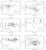 |
Fig. 11 Oxygen gas abundance and stellar metallicities relative to solar as a function of the logarithm of galactocentric radius in arcsec. R = 0 is shifted to log R = −0.5. Asterisks indicate metallicities relative to solar obtained from the stellar population (see text for details). Open squares indicate oxygen gas abundances using R23 for run2 galaxies, and error bars cover values obtained with all methods but O2Ne3. Fon run1 galaxies, open squares indicate those obtained with O3N2, diamonds with N2, and triangles with SB1. Galaxies hosting AGN are marked, with the vertical lines indicating the region affected by the active nuclei (either as in Fig. 7 or 3′′, as indicated in references in Véron-Cetty & Véron (2006)). |
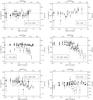 |
Fig. 11 continued. |
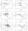 |
Fig. 11 continued. |
The bar position angles were derived using the Digital Sky Survey (DSS) images.
Acknowledgments
We are grateful to the referee for the useful comments and suggestions that have improved the manuscript. We acknowledge the usage of the HyperLeda database (http://leda.univ-lyon1.fr). This research has been supported by the Spanish Ministry of Science and Innovation (MICINN) under grants AYA2011-24728, AYA2010-21322-C03-02, AYA2010-21322-C03-03, AYA2007-67625-C02-02 and Consolider-Ingenio CSD2010-00064, and by the Junta de Andalucía (FQM-108). P.S.B. acknowledge support from the Ramon y Cajal Program financed by the Spanish Ministry of Science and Innovation. P.S.B. also acknowledges an ERC grant within the 6th European Community Framework Programme.
References
- Allen de Prieto, C., Lambert, D. L., & Asplund, M. 2001, ApJ, 556, L63 [NASA ADS] [CrossRef] [Google Scholar]
- Alloin, D., Edmunds, M. G., Lindblad, P. O., & Pagel, B. E. J. 1981, A&A, 101, 377 [NASA ADS] [Google Scholar]
- Annibali, F., Bressan, A., Rampazzo, R., Zeilinger, W. W., & Danese, L. 2007, A&A, 463, 455 [NASA ADS] [CrossRef] [EDP Sciences] [Google Scholar]
- Annibali, F., Bressan, A., Rampazzo, R., et al. 2010, A&A, 519, A40 [NASA ADS] [CrossRef] [EDP Sciences] [Google Scholar]
- Athanassoula, E. 1992, Physics of Nearby Galaxies: Nature or Nurture?, Proc. 27th Rencontre de Moriond, eds. T. X. Thuan, C. Balkowski, & J. Tran Thanh Van (Gif-sur-Yvette: Éd. Frontière), 505 [Google Scholar]
- Athanassoula, E. 2000, Stars, Gas and Dust in Galaxies: Exploring the Links, 221, 243 [Google Scholar]
- Athanassoula, L. 2003, Galaxies and Chaos, 626, 313 [NASA ADS] [CrossRef] [Google Scholar]
- Athey, A. E., & Bregman, J. N. 2009, ApJ, 696, 681 [NASA ADS] [CrossRef] [Google Scholar]
- Baldwin, J. A., Phillips, M. M., & Terlevich, R. 1981, PASP, 93, 5 [NASA ADS] [CrossRef] [EDP Sciences] [Google Scholar]
- Balser, D. S., Rood, R. T., Bania, T. M., & Anderson, L. D. 2011, BAAS, 43, #132.03 [Google Scholar]
- Block, D. L., Puerari, I., Knapen, J. H., et al. 2001, A&A, 375, 761 [NASA ADS] [CrossRef] [EDP Sciences] [Google Scholar]
- Block, D. L., Buta, R., Knapen, J. H., et al. 2004, AJ, 128, 183 [NASA ADS] [CrossRef] [Google Scholar]
- Bresolin, F. 2007, ApJ, 656, 186 [NASA ADS] [CrossRef] [Google Scholar]
- Bresolin, F., Ryan-Weber, E., Kennicutt, R. C., & Goddard, Q. 2009, ApJ, 695, 580 [NASA ADS] [CrossRef] [Google Scholar]
- Buta, R. 1986, ApJS, 61, 609 [NASA ADS] [CrossRef] [Google Scholar]
- Buta, R., Laurikainen, E., Salo, H., Block, D. L., & Knapen, J. H. 2006, AJ, 132, 1859 [NASA ADS] [CrossRef] [Google Scholar]
- Cardiel, N. 1999, Ph.D. Thesis [Google Scholar]
- Castellanos, M., Díaz, A. I., & Terlevich, E. 2002, MNRAS, 329, 315 [NASA ADS] [CrossRef] [Google Scholar]
- Chiappini, C., Matteucci, F., & Padoan, P. 2000, ApJ, 528, 711 [NASA ADS] [CrossRef] [Google Scholar]
- Colavitti, E., Matteucci, F., & Murante, G. 2008, A&A, 483, 401 [NASA ADS] [CrossRef] [EDP Sciences] [Google Scholar]
- Considère, S., Coziol, R., Contini, T., & Davoust, E. 2000, A&A, 356, 89 [NASA ADS] [Google Scholar]
- Davis, T. A., Alatalo, K., Sarzi, M., et al. 2011, MNRAS, 1497 [Google Scholar]
- Denicoló, G., Terlevich, R., & Terlevich, E. 2002, MNRAS, 330, 69 [NASA ADS] [CrossRef] [Google Scholar]
- Dopita, M. A., & Evans, I. N. 1986, ApJ, 307, 431 [NASA ADS] [CrossRef] [Google Scholar]
- Edmunds, M. G., & Pagel, B. E. J. 1984, MNRAS, 211, 507 [NASA ADS] [CrossRef] [Google Scholar]
- Edmunds, M. G., & Roy, J.-R. 1993, MNRAS, 261, L17 [NASA ADS] [CrossRef] [Google Scholar]
- Edvardsson, B. 2002, Cosmic Chemical Evolution, 187, 91 [NASA ADS] [CrossRef] [Google Scholar]
- Ellison, S. L., Nair, P., Patton, D. R., et al. 2011, MNRAS, 416, 2182 [NASA ADS] [CrossRef] [Google Scholar]
- Erwin, P. 2004, A&A, 415, 941 [NASA ADS] [CrossRef] [EDP Sciences] [Google Scholar]
- Filippenko, A. V. 1982, PASP, 94, 715 [NASA ADS] [CrossRef] [Google Scholar]
- Friedli, D. 1999, The Evolution of Galaxies on Cosmological Timescales, 187, 88 [NASA ADS] [Google Scholar]
- Friedli, D., & Benz, W. 1995, A&A, 301, 649 [NASA ADS] [Google Scholar]
- Friedli, D., Benz, W., & Kennicutt, R. 1994, ApJ, 430, L105 [NASA ADS] [CrossRef] [Google Scholar]
- Garnett, D. R., & Shields, G. A. 1987, ApJ, 317, 82 [NASA ADS] [CrossRef] [Google Scholar]
- Goddard, Q. E., Bresolin, F., Kennicutt, R. C., Ryan-Weber, E. V., & Rosales-Ortega, F. F. 2011, MNRAS, 412, 1246 [NASA ADS] [Google Scholar]
- Hidalgo-Gámez, A. M., Ramírez-Fuentes, D., & González, J. J. 2011, AJ, in press [Google Scholar]
- Howarth, I. D. 1984, MNRAS, 203, 301 [Google Scholar]
- Hummer, D. G., & Storey, P. J. 1987, MNRAS, 224, 801 [NASA ADS] [CrossRef] [Google Scholar]
- Kauffmann, G., Heckman, T. M., Tremonti, C., et al. 2003, MNRAS, 346, 1055 [Google Scholar]
- Jungwiert, B., Combes, F., & Axon, D. J. 1997, A&AS, 125, 479 [NASA ADS] [CrossRef] [EDP Sciences] [Google Scholar]
- Kennicutt, R. C., Keel, W. C., & Blaha, C. A. 1989, AJ, 97, 1022 [NASA ADS] [CrossRef] [Google Scholar]
- Kennicutt, R. C., Bresolin, F., & Garnett, D. R. 2003, ApJ, 2009, 748 [Google Scholar]
- Kereš, D., Katz, N., Weinberg, D. H., & Davé, R. 2005, MNRAS, 363, 2 [NASA ADS] [CrossRef] [Google Scholar]
- Kewley, L. J., & Dopita, M. A. 2002, ApJS, 142, 35 [NASA ADS] [CrossRef] [Google Scholar]
- Kewley, L. J., & Ellison, S. L. 2008, ApJ, 681, 1183 [NASA ADS] [CrossRef] [Google Scholar]
- Kewley, L. J., Dopita, M. A., Sutherland, R. S., Heisler, C. A., & Trevena, J. 2001, ApJ, 556, 121 [Google Scholar]
- Kewley, L. J., Groves, B., Kauffmann, G., & Heckman, T. 2006, MNRAS, 372, 961 [NASA ADS] [CrossRef] [Google Scholar]
- Kobulnicky, H. A., Kennicutt, R. C., Jr., & Pizagno, J. L. 1999, ApJ, 514, 544 [NASA ADS] [CrossRef] [Google Scholar]
- Laurikainen, E., Salo, H., Buta, R., & Vasylyev, S. 2004, MNRAS, 355, 1251 [NASA ADS] [CrossRef] [Google Scholar]
- Lindblad, P.-O., & Fathi, K. 2011, in Tracing the Ancestry of Galaxies (on the land our ancestors), Proc. International Astronomical Union (Cambridge University Press), IAU Symp., 277, 191 [Google Scholar]
- López-Sánchez, Á. R., & Esteban, C. 2010, A&A, 517, A85 [NASA ADS] [CrossRef] [EDP Sciences] [Google Scholar]
- MacArthur, L. A., González, J. J., & Courteau, S. 2009, MNRAS, 395, 28 [NASA ADS] [CrossRef] [Google Scholar]
- Marino, A., Rampazzo, R., Bianchi, L., et al. 2011, MNRAS, 411, 311 [NASA ADS] [CrossRef] [Google Scholar]
- Márquez, I., Masegosa, J., Moles, M., et al. 2002, A&A, 393, 389 [NASA ADS] [CrossRef] [EDP Sciences] [Google Scholar]
- Martin, P. 1992, Ph.D. Thesis [Google Scholar]
- Martin, P., & Friedli, D. 1997, A&A, 326, 449 [NASA ADS] [Google Scholar]
- Martin, P., & Roy, J.-R. 1995, ApJ, 445, 161 [NASA ADS] [CrossRef] [Google Scholar]
- McCall, M. L., Rybski, P. M., & Shields, G. A. 1985, ApJSS, 57, 1 [NASA ADS] [CrossRef] [Google Scholar]
- McGaugh, S. S. 1991, ApJ, 380, 140 [NASA ADS] [CrossRef] [Google Scholar]
- Moiseev, A. V. 2001, BSAO, 51, 140 [Google Scholar]
- Moustakas, J., Kennicutt, R. C., Jr., Tremonti, C. A., et al. 2010, ApJS, 190, 233 [NASA ADS] [CrossRef] [Google Scholar]
- Nagao, T., Maiolino, R., & Marconi, A. 2006, A&A, 459, 85 [NASA ADS] [CrossRef] [EDP Sciences] [Google Scholar]
- Oey, M. S., & Kennicutt, R. C. Jr. 1993, ApJ, 411, 137 [NASA ADS] [CrossRef] [Google Scholar]
- Osterbrock, D. E. 1989, Astrophysics of Gaseous Nebulae and Activa Galactic Nuclei (Mill Valley: University Science Books) [Google Scholar]
- Pagel, B. E. J., & Edmunds, M. G. 1981, ARA&A, 19, 77 [NASA ADS] [CrossRef] [Google Scholar]
- Pagel, B. E. J., Edmunds, M. G., Blackwell, D. E., Chun, M. S., & Smith, G. 1979, MNRAS, 189, 95 [NASA ADS] [CrossRef] [Google Scholar]
- Pérez, I., & Sánchez-Blázquez, P. 2011, A&A, 529, A64 (Paper II) [NASA ADS] [CrossRef] [EDP Sciences] [Google Scholar]
- Pérez, I., Sánchez-Blázquez, P., & Zurita, A. 2007, A&A, 465, L9 [NASA ADS] [CrossRef] [EDP Sciences] [Google Scholar]
- Pérez, I., Sánchez-Blázquez, P., & Zurita, A. 2009, A&A, 495, 775 (Paper I) [NASA ADS] [CrossRef] [EDP Sciences] [Google Scholar]
- Pérez-Montero, E., Hägele, G. F., Contini, T., & Díaz, A. I. 2007, MNRAS, 381, 125 [NASA ADS] [CrossRef] [Google Scholar]
- Pettini, M., & Pagel, B. E. J. 2004, MNRAS, 348, L59 [NASA ADS] [CrossRef] [Google Scholar]
- Pfenniger, D., & Friedli, D. 1991, A&A, 252, 75 [NASA ADS] [Google Scholar]
- Phillips, A. C. 1993, BAAS, 25, 1329 [NASA ADS] [Google Scholar]
- Pilyugin, L. S. 2000, A&A, 362, 325 [NASA ADS] [Google Scholar]
- Pilyugin, L. S. 2001, A&A, 369, 594 [NASA ADS] [CrossRef] [EDP Sciences] [Google Scholar]
- Pilyugin, L. S., & Thuan, T. X. 2005, ApJ, 631, 231 [NASA ADS] [CrossRef] [MathSciNet] [Google Scholar]
- Portinari, L., & Chiosi, C. 1999, A&A, 350, 827 [NASA ADS] [Google Scholar]
- Prantzos, N. 2008, EAS Publ. Ser., 32, 311 [CrossRef] [EDP Sciences] [Google Scholar]
- Rola, C. S., Terlevich, E., & Terlevich, R. J. 1997, MNRAS, 289, 419 [NASA ADS] [Google Scholar]
- Roškar, R., Debattista, V. P., Stinson, G. S., et al. 2008, Formation and Evolution of Galaxy Disks, 396, 217 [NASA ADS] [Google Scholar]
- Rupke, D. S. N., Kewley, L. J., & Barnes, J. E. 2010, ApJ, 710, L156 [NASA ADS] [CrossRef] [Google Scholar]
- Sánchez-Blázquez, P., Peletier, R. F., Jiménez-Vicente, J., et al. 2006, MNRAS, 371, 703 [NASA ADS] [CrossRef] [Google Scholar]
- Sánchez-Blázquez, P., Gibson, B. K., Kawata, D., Cardiel, N., & Balcells, M. 2009, MNRAS, 400, 1264 [NASA ADS] [CrossRef] [Google Scholar]
- Sanchez-Blazquez, P., Ocvirk, P., Gibson, B. K., Perez, I., & Peletier, R. F. 2011, MNRAS, 415, 709 [NASA ADS] [CrossRef] [Google Scholar]
- Sarzi, M., Rix, H.-W., Shields, J. C., et al. 2005, ApJ, 628, 169 [NASA ADS] [CrossRef] [Google Scholar]
- Seaton, M. J. 1979, MNRAS, 187, 73P [NASA ADS] [CrossRef] [Google Scholar]
- Schönrich, R., & Binney, J. 2009, MNRAS, 399, 1145 [NASA ADS] [CrossRef] [Google Scholar]
- Storchi-Bergmann, T., Calzetti, D., & Kinney, A. L. 1994, ApJ, 429, 572 [NASA ADS] [CrossRef] [Google Scholar]
- Storchi-Bergmann, T., Schmitt, H. R., Calzetti, D., & Kinney, A. L. 1998, AJ, 115, 909 [NASA ADS] [CrossRef] [Google Scholar]
- Tremonti, C. A., Heckman, T. M., Kauffmann, G., et al. 2004, ApJ, 613, 898 [NASA ADS] [CrossRef] [Google Scholar]
- van Zee, L., Salzer, J. J., Haynes, M. P., O’Donoghue, A. A., & Balonek, T. J. 1998, AJ, 116, 2805 [NASA ADS] [CrossRef] [Google Scholar]
- Vazdekis, A., Sánchez-Blázquez, P., Falcón-Barroso, J., et al. 2010, MNRAS, 404, 1639 [NASA ADS] [Google Scholar]
- Veilleux, S., & Osterbrock, D. E. 1987, ApJS, 63, 295 [NASA ADS] [CrossRef] [Google Scholar]
- Verley, S., Combes, F., Verdes-Montenegro, L., Bergond, G., & Leon, S. 2007, A&A, 474, 43 [NASA ADS] [CrossRef] [EDP Sciences] [Google Scholar]
- Véron-Cetty, M.-P., & Véron, P. 2006, A&A, 455, 773 [NASA ADS] [CrossRef] [EDP Sciences] [Google Scholar]
- Vila-Costas, M. B., & Edmunds, M. G. 1992, MNRAS, 252, 121 [NASA ADS] [CrossRef] [Google Scholar]
- Wozniak, H., Friedli, D., Martinet, L., Martin, P., & Bratschi, P. 1995, A&AS, 111, 115 [NASA ADS] [Google Scholar]
- Yates, R. M., Kauffmann, G., & Guo, Q. 2012, MNRAS, 422, 215 [NASA ADS] [CrossRef] [Google Scholar]
- Yoachim, P., & Dalcanton, J. J. 2008, ApJ, 682, 1004 [NASA ADS] [CrossRef] [Google Scholar]
- Zahid, H. J., & Bresolin, F. 2011, AJ, 141, 192 [NASA ADS] [CrossRef] [Google Scholar]
- Zaritsky, D., Kennicutt, R. C. Jr., & Huchra, J. P. 1994, ApJ, 420, 87 [NASA ADS] [CrossRef] [Google Scholar]
All Tables
Oxygen abundance gradients for all adopted methods and the central abundance, for run2 galaxies.
Metallicity gradients in the bulge regions with all the adopted methods for run2 galaxies, including AGN-affected regions.
Metallicity gradients in the bulge regions, with all the used methods, for run1 galaxies, including AGN regions.
All Figures
|
Fig. 1 Central spectrum for NGC 1169 (from run2). The top panel shows the observed spectrum (yellow line) and the fitted template (black line). Bottom panel shows the residuals from the fit. Oxygen and Hβ lines are clearly visible. |
| In the text | |
|
Fig. 2 Central spectrum for NGC 2273 (run2). Panels are the same as in Fig. 1. In this spectrum, the [Ne iii]λ3868 line can be clearly identified. |
| In the text | |
|
Fig. 3 Blue and red central spectra for NGC 3081 (run1). In the top panels, observed spectra (yellow lines) and templates (black lines) are shown. Bottom panels show the residuals of the fit. |
| In the text | |
|
Fig. 4 Diagnostic diagram for the emission-line regions of run1 galaxies at different galactocentric distances (R) scaled with R25. The solid line (Kewley et al. 2001) sets the star formation upper limit, the dashed line (Kauffmann et al. 2003) the empirical division between star-forming galaxies (SF) and transition objects (T), and the horizontal line (Kewley et al. 2006) separates Seyferts and Low-Ionization Nuclear Emission-line Regions (LINERs). |
| In the text | |
|
Fig. 5 Diagnostic diagram for the emission-line regions of run1 galaxies for different galactocentric distances (R) scaled with R25. The solid line delineates our adopted separation between star formation regions and AGNs; below the dashed line there are LINERs and above it Seyferts (Kewley et al. 2006). |
| In the text | |
|
Fig. 6 Diagnostic diagram for those galaxies in which we have detected the [Ne iii]λ3869 line. The solid line indicates the limit between star-formation regions and AGNs, and the dashed one between LINERs ([O iii]5007/Hβ ≤ 0.5) and Seyferts 2 ([O iii]5007/Hβ > 0.5) (Rola et al. 1997). |
| In the text | |
|
Fig. 7 Radial distribution of log ([O iii]/Hβ) (for active galaxies of run1) and log ([Ne iii]/Hβ) (for run2 galaxies with [Ne iii]λ3869 line detected). The theoretical curves of Kewley et al. (2001, for log ([O iii]/Hβ) and log ([N ii]/Hα)) and Rola et al. (1997, for log ([Ne iii]/Hβ)) distinguishing between AGN and SF are also plotted with dashed and solid lines, respectively. |
| In the text | |
|
Fig. 8 Relation between different calibrations for obtaining oxygen abundances. In panels a) − d), we compare the methods used for run2 galaxies with the R23 calibration by McGaugh (M91). In panels e) and f), the comparison is for run1 galaxies, between N2 and either O3N2 or SB1. The solid line in each plot shows the agreement between the different methods. |
| In the text | |
|
Fig. 9 Differences between the oxygen abundances obtained with the different methods versus the galactocentric radius for each galaxy. R25 has been taken from HyperLeda. Residuals are with respect to R23 (M91) for run2 galaxies and to N2 for run1 galaxies. Crosses are oxygen abundances obtained from the O2Ne3 calibration, triangles from R23 (Z94), circles from KD03, squares from P05, diamonds from O3N2, and asterisks from SB1. |
| In the text | |
|
Fig. 10 Oxygen abundances of 12 + log (O/H) obtained with O3N2 for run1, and with R23 (M91) for run2, versus R/R25 in each galaxy. Dashed lines indicate the fits to all measured values, and solid lines show the best fits within the bulge region. For run1 galaxies, black lines indicate the N2 fit, cyan lines the O3N2 fit, and blue line the SB1 fit. For run2 galaxies, black lines show the R23 (M91) fit, blue lines the Z94 fit, green lines the KD03 fit, and red lines the P05 fit. |
| In the text | |
|
Fig. 10 continued. |
| In the text | |
|
Fig. 12 Comparison of the metallicity gradients obtained for the gaseous and stellar components in the bar region of our sample galaxies. They are normalized to R25 (i.e. the gradients have been obtained from linear fits to the 12 + log (O/H) versus R/R25 representation for each galaxy). Circles are those estimated with the R23 (M91) or N2 methods, squares are the mean value of gradients calculated with all methods (the error bar covers the range of these gradients), and stars are the gradient [Z/H] for the stellar component (Paper II). Order indicated along the abscissas is that of Tables 6 and 7. Filled symbols represent star-forming galaxies. |
| In the text | |
|
Fig. 13 Comparation between metallicity gradients obtained for gaseous and stellar components in the bulge region of our sample galaxies. They are normalized to R25 (i.e. the gradients have been obtained from linear fits to the 12 + log (O/H) versus R/R25 representation for each galaxy). Circles are those estimated with the R23 (M91) or N2 methods, squares are the mean value of gradients calculated with all methods (the error bar covers the range of these gradients), and stars are the gradient [Z/H] for the stellar component (Paper II). The order along the abscissas is that of Tables 6 and 7. Filled symbols represent star-forming galaxies. |
| In the text | |
|
Fig. 14 Rotational velocity corrected for inclination versus central oxygen abundances (1.2 arcsec). Filled circles represent those calculated using the R23 method for run2 and O3N2 for run1. Squares are values obtained with N2 for run1. |
| In the text | |
|
Fig. 15 Stellar velocity dispersion versus central oxygen abundances (1.2 arcsec). Filled circles represent those calculated using the R23 method for run2 and O3N2 for run1. Squares are values obtained with N2 for run1. |
| In the text | |
|
Fig. 11 Oxygen gas abundance and stellar metallicities relative to solar as a function of the logarithm of galactocentric radius in arcsec. R = 0 is shifted to log R = −0.5. Asterisks indicate metallicities relative to solar obtained from the stellar population (see text for details). Open squares indicate oxygen gas abundances using R23 for run2 galaxies, and error bars cover values obtained with all methods but O2Ne3. Fon run1 galaxies, open squares indicate those obtained with O3N2, diamonds with N2, and triangles with SB1. Galaxies hosting AGN are marked, with the vertical lines indicating the region affected by the active nuclei (either as in Fig. 7 or 3′′, as indicated in references in Véron-Cetty & Véron (2006)). |
| In the text | |
|
Fig. 11 continued. |
| In the text | |
|
Fig. 11 continued. |
| In the text | |
Current usage metrics show cumulative count of Article Views (full-text article views including HTML views, PDF and ePub downloads, according to the available data) and Abstracts Views on Vision4Press platform.
Data correspond to usage on the plateform after 2015. The current usage metrics is available 48-96 hours after online publication and is updated daily on week days.
Initial download of the metrics may take a while.