| Issue |
A&A
Volume 542, June 2012
|
|
|---|---|---|
| Article Number | A6 | |
| Number of page(s) | 11 | |
| Section | Interstellar and circumstellar matter | |
| DOI | https://doi.org/10.1051/0004-6361/201118582 | |
| Published online | 24 May 2012 | |
Extended warm and dense gas towards W49A: starburst conditions in our Galaxy?
1 Kapteyn Astronomical Institute, University of Groningen, PO Box 800, 9700 AV Groningen, The Netherlands
e-mail: This email address is being protected from spambots. You need JavaScript enabled to view it.
2 SRON Netherlands Institute for Space Research, PO Box 800, 9700 AV Groningen, The Netherlands
3 Jodrell Bank Centre for Astrophysics, School of Physics and Astronomy, University of Manchester, Manchester, M13 9PL, UK
4 Department of Physics and Astronomy, University of Calgary, Calgary, T2N 1N4, AB, Canada
Received: 5 December 2011
Accepted: 28 March 2000
Abstract
Context. The star formation rates in starburst galaxies are orders of magnitude higher than in local star-forming regions, and the origin of this difference is not well understood.
Aims. We use sub-mm spectral line maps to characterize the physical conditions of the molecular gas in the luminous Galactic star-forming region W49A and compare them with the conditions in starburst galaxies.
Methods. We probe the temperature and density structure of W49A using H2CO and HCN line ratios over a 2′ × 2′ (6.6 × 6.6 pc) field with an angular resolution of 15′′ (~0.8 pc) provided by the JCMT Spectral Legacy Survey. We analyze the rotation diagrams of lines with multiple transitions with corrections for optical depth and beam dilution, and estimate excitation temperatures and column densities.
Results. Comparing the observed line intensity ratios with non-LTE radiative transfer models, our results reveal an extended region (about 1′ × 1′, equivalent to ~3 × 3 pc at the distance of W49A) of warm (>100 K) and dense (> 105 cm-3) molecular gas, with a mass of 2 × 10⁴ − 2 × 10⁵ M⊙ (by applying abundances derived for other regions of massive star-formation). These temperatures and densities in W49A are comparable to those found in clouds near the center of the Milky Way and in starburst galaxies.
Conclusions. The highly excited gas is likely to be heated via shocks from the stellar winds of embedded, O-type stars or alternatively due to UV irradiation, or possibly a combination of these two processes. Cosmic rays, X-ray irradiation and gas-grain collisional heating are less likely to be the source of the heating in the case of W49A.
Key words: stars: formation / ISM: molecules / ISM: individual objects: W49A
© ESO, 2012
1. Introduction
The formation of stars proceeds on scales ranging from 1000 AU-sized isolated low-mass cores to ~10 pc-sized giant molecular clouds with embedded massive clusters. The observed levels of star-formation activity also vary greatly: from ~10-4 M⊙/yr in dwarf galaxies like I Zw 18 (Aloisi et al. 1999) to ~3 M⊙/yr in the Milky Way to ~103 M⊙/yr in starburst galaxies (e.g. Solomon & Vanden Bout 2005). The origin of this large spread in star formation rate may lie in different physical conditions with the gas forming the stars, the nature and role of feedback effects or other mechanisms. As one of the the most active star-forming regions in the Galactic disk, W49A provides a relatively nearby laboratory in which to study intense star formation activity and may provide insights into explaining the large observed range in star-formation activity in galaxies.
W49A is a luminous (>107 L⊙) and massive (~106 M⊙) star-forming region (Sievers et al. 1991) at a distance of 11.4 kpc (Gwinn et al. 1992). W49A contains several signatures of high star-formation activity, in particular, strong H2O maser emission (Genzel et al. 1978). Line ratios of HNC, HCN and HCO+ and their isotopologues suggest similar conditions to starburst galaxies (Roberts et al. 2011). Several ideas have been proposed to explain the high star-formation activity of W49A.
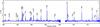 |
Fig. 1 The spectrum towards the source center (RA(J2000) = 19:10:13.4; Dec(J2000) = 09:06:14) in the 360−373 GHz frequency range of the SLS. The main detected lines are labeled. The gap in the spectrum around 368.5 GHz is a region of high atmospheric extinction and was not observed. |
Welch et al. (1987) propose a large-scale inside-out gravitational collapse by interpreting two velocity components of HCO+J = 1–0 spectra measured toward the ring-like configuration of UC Hii regions in terms of an infall profile. Serabyn et al. (1993) interpret the two-components of the double-peak line profile seen in CS (J = 10–9, 7−6, 5−4, 3−2) and C34S (J = 10–9, 7−6, 5−4) transitions as coming from different clouds, and suggest that massive star formation in W49A is triggered by a large-scale cloud merger. Williams et al. (2004) argue that one cannot distinguish between a global collapse model of a large cloud and a multiple-cloud model, based on HCO+ (J = 3–2 and 1−0) and C18O (J = 2–1) data. Roberts et al. (2011) observe single-peaked HC18O+ (J = 4–3) line profiles, which supports the large-scale infall hypothesis. In 13CO and C18O J = 2–1 maps of the W49A region Peng et al. (2010) find evidence of expanding shells with the dense clumps in the region lying peripherally along the shells. These expanding shells could provide a natural explanation of the observed molecular line profiles, and triggered massive star formation in W49A.
This paper reports new kinetic temperature and density estimates for a 2′ × 2′ region of W49A based on single dish, JCMT images with 15′′ resolution. These indicate the presence of extended warm and dense gas towards the central region of the source. We use these results to compare W49A to starburst galaxies where similar results have been reported.
2. Observations and data reduction
This paper presents results from data obtained as part of the JCMT Spectral Legacy Survey (SLS, Plume et al. 2007) covering between 330 and 373 GHz which has been carried out at the James Clerk Maxwell Telescope (JCMT)1 on Mauna Kea, Hawai’i. The data were taken using the HARP-B receiver and the ACSIS correlator (Buckle et al. 2009). HARP-B consists of 16 pixels or receptors separated by 30 arcsec with a foot print of 2 arcmin.
The observations were carried out using jiggle-position switch mode. Each map covers a 2′ × 2′ field sampled every 7.5′′, half of the JCMT beam width at the relevant frequencies (15′′ at 345 GHz). The spectral resolution at these frequencies is ~0.8 km s-1 and the beam efficiency is 0.63 (Buckle et al. 2009). The spectra were taken using an off-position 14′ to the northeast of the source.
Data reduction was done manually using the tools in the Starlink software package. The raw time series files are processed in 1 GHz wide chunks. These files were inspected for bad receptors, baselines and frequency spikes. Bad receptors, bad baselines and spikes were masked in the time series files before they have been converted to three-dimensional data cubes (RA × Dec × frequency). These 3D cubes then were baseline corrected by fitting and removing a linear or second-order polynomial baseline. The baseline corrected cubes are then mosaicked to a larger cube covering an area of 2′ × 2′ and the frequency range of interest. Single sideband system temperatures for these observations are in the range between 255 K (at 360 GHz) and 700 K (at 373 GHz). The analysis here primarily focuses on a number of spectral lines in the 360 − 373 GHz range plus a few selected lines from the 330 − 360 GHz part of the survey. The whole, systematic data analysis of the full SLS frequency range is the focus of a future paper.
We also use ancillary observations of the HCN J = 3–2 transition made using JCMT raster maps with half-beamwidth spacing using the receiver A (211 − 276 GHz; beamwidth 20′′; main beam efficiency: 0.69). The HCN 3 − 2 map covers approximately the same field that of the SLS HARP maps. The HCN 3 − 2 data were reduced and calibrated with standard Starlink procedures. Linear baselines were removed and the data were Hanning smoothed. The map is a grid of 15 pixel × 15 pixels, where each pixel covers 8′′ × 8′′.
Summary of the molecular lines used in this paper.
3. Results
3.1. Line selection
Figure 1 shows the 360−373 GHz spectrum towards the central position (RA(J2000) = 19:10:13.4; Dec(J2000) = 09:06:14). More than 80 lines have been identified in this spectrum.
Our initial selection of lines for the analysis here is based on molecules that show multiple transitions in the high-frequency range (360 − 373 GHz) of the SLS, which include six H2CO, five CH3OH and nine SO2 transitions (Table 1). These are used to trace the excitation conditions. One more H2CO transition from the lower frequency part of the survey (H2CO 515−414) was added to be used as a tracer of kinetic temperatures, together with the 533−432 transition from the high-frequency part of the SLS. The HCN 4−3 transition was selected from the lower frequency range, to trace the density structure, together with the HCN 3 − 2 transition.
In this paper, we restrict our analysis to our line selection summarized above and in Table 1. A subsequent paper (Nagy et al., in prep.) will give more details on the chemical inventory including the full SLS frequency range (330 − 373 GHz) and on kinematics traced by various species with significant spatial extension. Figure 2 shows the main regions around the center of W49A overplotted on the integrated intensity maps in the HCN 4−3, SO2 152,14−141,13, CH3OH 72,5 − 61,5 and H2CO 515−414 lines. The integrated intensities of the HCN and H2CO lines show a similar distribution, indicating that their emission originates in the same volume. This is also supported by the line profiles of these two species (Nagy et al., in prep.). In the following sections, we will refer to these regions with the coordinates indicated in the figure: source center (RA(J2000) = 19:10:13.4; Dec(J2000) = 09:06:14), eastern tail (RA(J2000) = 19:10:16.6; Dec(J2000) = 09:05:48), northern clump (RA(J2000) = 19:10:13.6; Dec(J2000) = 09:06:48) and southwest clump (RA(J2000) = 19:10:10.6; Dec(J2000) = 09:05:18).
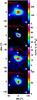 |
Fig. 2 The integrated intensity distribution of HCN 4−3, SO2 152,14−141,13, CH3OH 72,5−61,5 and H2CO 515−414. The central position is shown with black plus signs, the off-center regions (northern clump, eastern tail and southwest clump) are also shown with white plus signs. |
3.2. Excitation conditions
A well known method for the estimation of excitation temperatures and column densities is the rotational diagram method (e.g. Turner 1991). It can be applied to molecules with multiple observed transitions using three assumptions: 1) the lines are optically thin, 2) the level populations can be characterized by a single excitation temperature (“rotational temperature”, Trot) and 3) the emission is homogeneous and fills the telescope beam. Then the measured integrated main-beam temperatures of lines ( K km s-1) is related to the column densities of the molecules in the upper level (Nu) by:
 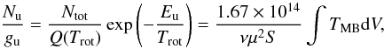 (1)with gu the statistical weight of level u, Ntot the total column density in cm-2, Q(Trot) the partition function for Trot, Eu the upper level energy in K, ν the frequency in GHz, μ the permanent dipole moment in Debye and S the line strength value. A linear fit to ln(Nu/gu) – Eu gives Trot as the inverse of the slope, and Ntot, the column density can be derived. The rotational temperature would be expected to be equal to the kinetic temperatures if all levels were thermalized.
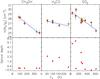 |
Fig. 3 The results of the rotation diagram analysis for H2CO toward the center. Top panels: the results of the rotation diagram analysis before (red symbols) and after (green symbols) corrections for optical depth and beam dilution. The overplotted blue line corresponds to a linear fit to the rotational diagram without corrections. Bottom panels: the corresponding best fit optical depths from the χ2 minimization. |
Results of the excitation analysis toward the center of W49A.
In the case of non-LTE excitation, a different excitation temperature may characterize the population of each level relative to that of the ground state or relative to that of any other level. In this case, the three assumptions mentioned for the rotation diagram method do not apply. Equation (1) can be modified to include the effect of optical depth τ through the factor Cτ = τ/(1 − e − τ) and beam dilution f ( = Ωs/Ωa) (Goldsmith & Langer 1999), with Ωs the size of the emission region and Ωa the size of the telescope beam.  (2)According to Eq. (2), for a given upper level, Nu can be evaluated from a set of Ntot,1, Tex, f and Cτ. Since Cτ is a function of Ntot,1 and Tex, the independent parameters are therefore Ntot,1, Tex and f. Solving the equation for a “source size” between 1″ and 15″ (which is equivalent with a beam dilution factor between (1/15)2 and uniform beam filling), χ2 minimization gives Ntot,1 and Tex. Figure 3 shows the rotation diagrams for CH3OH, H2CO & SO2 toward the central position with (green symbols) and without (red symbols) taking into account the optical depth and beam dilution. Table 2 includes the parameters of the rotation diagram fit toward the central position.
The CH3OH lines are found to be optically thin (τ = 0.004 − 0.02), so the rotation diagram fit is a good approximation to the column densities and excitation temperatures. The derived rotation temperature is 83 ± 7 K. The H2CO and SO2 lines are mostly optically thick with optical depths in the range of 0.2−2.35 for H2CO and 0.1−5.4 for SO2. The best fit excitation temperatures are 138 K for H2CO and 115 K for SO2. The best fit total column densities are 4.3 × 1016 cm-2 for H2CO and 1.4 × 1018 cm-2 for SO2. The χ2 minimization for H2CO and SO2 results in a best fit “source size” of ~2−3′′, which is equivalent with 0.11−0.17 pc for W49A. This is consistent with the sizes of hot cores and UC Hii regions resolved by sub-arcsecond resolution measurements, such as Wilner et al. (2001), De Pree et al. (1997, 2004).
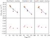 |
Fig. 4 The results of the rotation diagram analysis for H2CO at off-center positions. Top panels: the results of the rotation diagram analysis before (red symbols) and after (green symbols) corrections for optical depth and beam dilution. The overplotted blue line corresponds to a linear fit to the rotational diagram without corrections. Bottom panels: the corresponding best fit optical depths from the χ2 minimization. |
Results of the excitation analysis toward the off-center regions of W49A.
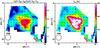 |
Fig. 5 Left panel: ratio of 533−432 to the 515−414 H2CO transition. Right panel: kinetic temperature map of W49A determined from line ratio shown in the left panel. |
Figure 4 shows the rotation diagrams for H2CO toward the three main regions outside the center. The rotation diagram with corrections for optical depth and beam dilution (Fig. 4 and Table 3) gives similar excitation conditions toward the three main sub-regions (excitation temperatures: 67 K for the northern clump, 56 K for the eastern tail and 61 K for the southwest clump). These excitation temperatures are about half of the excitation temperature towards the central position (138 K). Since the lines are optically thin, the rotation temperatures are good estimates for the excitation temperatures. The best fit column densities are also similar between the off-center positions, about 1.7−2.2 × 1013 cm-3, almost three orders of magnitude less than the best fit column density towards the center. The data at these positions are consistent with optically thin emission and uniform beam filling.
3.3. Kinetic temperature estimates
To estimate the local physical conditions in W49A, we use ratios of lines from the same molecular species. The kinetic temperature can be probed by the line ratios of H2CO lines from the same J-state but different K-states. In this case, we use the o-H2CO 515−414 (351.769 GHz) and o-H2CO 533−432 (364.275 GHz) transitions, since they have been detected in a large part of the SLS field and have been found to be excellent tracers of kinetic temperature (Fig. A.1). Our calculations use the non-LTE radiative transfer program Radex (Van der Tak et al. 2007), molecular data file from the LAMDA database (Schöier et al. 2005) and H2CO collision data from Green (1991), which have been scaled by 1.37 to make a first order approximation for collisions with H2. Uncertainties introduced by using these rates may be up to 50% for the column densities, but less affect the densities and temperatures, since those are derived from line intensity ratios. More recent calculations by Troscompt et al. (2009) are more accurate, however, include a more limited range of temperatures and transitions, therefore, were not used in our calculations.
Figure A.1 shows the calculated line ratios as a function of kinetic temperature and H2 density. In the central 40′′ × 40′′ region, FWHM = 12 km s-1 was used as an initial parameter for Radex, while outside of this region we used FWHM = 6 km s-1, based on the observed values. However, there is no strong dependence on the FWHM of the lines. We apply a molecular column density of N(H2CO) = 5 × 1014 cm-2 as an “average” value for all the positions over the SLS field. This is slightly below the value that can reproduce the optical depths derived from rotation diagram method for the central position, assuming uniform beam filling.
The results are shown in Fig. 5 with the main regions highlighted. We derive a kinetic temperature of 300 K toward the center, 98 K toward the northern clump, 85 K toward the southwest clump and 68 K toward the eastern tail, with an uncertainty of ~30%. In fact, there is a large, about 1′ × 1′ (~3 × 3 pc) region around the center, with kinetic temperatures ≳ 100 K.
3.4. Volume- and column density estimates
To estimate H2 volume densities of the high temperature gas that the H2CO line ratios trace, we use line ratios of the HCN 3 − 2 (265.886 GHz) and HCN 4−3 (354.505 GHz) transitions. Our calculations are based on collisional rates from Dumouchel et al. (2010), which have been scaled by a factor 1.37 to represent collisions with H2. The HCN 4−3 map has been convolved to the resolution of the HCN 3−2 map (20′′). Since the line ratios depend on the kinetic temperature (Fig. A.2), we use the kinetic temperatures determined from the H2CO line ratios to convert the measured HCN line ratios (Fig. 6) to volume densities. Therefore, even if HCN was detected towards almost the entire SLS field, our calculations only take into account the positions where both of the H2CO transitions were detected. The uncertainty of these density estimates is ~a factor of two. Figure 7 shows the estimated volume densities. Note that not all the positions with kinetic temperature estimates are included in the density map: this is due to the uncertainty of our method below 100 K, where the HCN 3−2/4−3 line ratios are rather temperature than density tracers. With a search range in the densities between 103 and 108 cm-3, an extended area towards the center (approximately corresponding to the high-excitation area revealed by the H2CO line ratios) corresponds to densities as high as 105 cm-3 or higher, with a maximum of 6.9 × 106 cm-3. The maximum density is measured toward an offset position compared to the position we refer to as “center”. The densities toward the central part show little less than an order of magnitude variation.
The average H2 volume density corresponding to the central 1 × 1 arcmin region is 1.6 × 106 cm-3. The lowest densities, toward the edges of the cloud area covered by our estimates, is a few times 104 cm-3. However, our density estimates are more accurate for densities between 105 and 108 cm-3 (Fig. A.2). In addition to the uncertainty of the method below ~105 cm-3, the H2CO 515−414 and 533−432 transitions are detected over a less extended region, compared to the HCN 3 − 2 and 4 − 3 transitions. Estimating the physical conditions outside the area covered by our kinetic temperature and volume density maps requires molecular line tracers with a larger spatial extent.
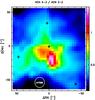 |
Fig. 6 Map of the line ratio of HCN J = 4 − 3 to HCN J = 3 − 2. |
Based on the kinetic temperatures and volume densities presented above, we estimate the column densities of the two main molecular tracers used in this paper, HCN and H2CO. These estimates use H2 volume densities of 1.8 × 106 cm-3 for the center, 1.2 × 106 cm-3 for the eastern tail, 5.6 × 105 cm-3 for the northern clump and 1.3 × 105 cm-3 for the southwest clump. The kinetic temperatures used for each position are listed in Sect. 3.3. To calculate the HCN column density toward the center, we use the H13CN 4 − 3 (345.3 GHz) transition, and 12C/13C = 77 (Wilson & Rood 1994). HCN peaks toward the center, with a column density of 7.3 × 1015 cm-2. The HCN column densities of the eastern tail and northern clump regions are comparable: N(HCN) = 7−8 × 1013 cm-2 toward the eastern tail and N(HCN) = 1.5−2 × 1014 cm-2 toward the northern clump. N(HCN) toward the southwest clump is a factor of 4 − 5 above the column density of the northern clump: N(HCN) = 6.2 − 9.6 × 1014 cm-2. N(H2CO) is ~ 3.2 × 10¹⁴ − 4.5 × 1014 cm-2 toward the center as well as the southwest clump. The northern clump has N(H2CO) slightly below the center and southwest clump, 7.0 × 10¹³ − 1.1 × 1014 cm-2, while toward the eastern tail, we measure a column density of 4.9 × 10¹³ − 5.0 × 1013 cm-2. The two orders of magnitude difference in the H2CO column density toward the center compared to the best fit column density derived from the rotation diagrams can be accounted for the simple assumption used in the rotation diagram method, that the level populations can be described by a single excitation temperature.
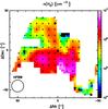 |
Fig. 7 Volume density estimates from the HCN 3 − 2 and HCN 4 − 3 lines. |
The mass of the warm and dense gas can be estimated based on the H2CO column density, by assuming an H2CO abundance. Van der Tak et al. (2000) derive H2CO abundances in the range of 10-9 − 10-10 for thirteen regions of massive star formation. For an “average” column density of 1014 cm-2 and an abundance of 10-9, the mass of the central 1′ × 1′ region with warm and dense gas is ~2 × 10⁴ M⊙, which becomes ~2 × 10⁵ M⊙ for an H2CO abundance of 10-10. These are comparable to the mass estimates based on dust continuum measurements. Ward-Thompson & Robson (1990) estimate a mass of ~2.4 × 10⁵M⊙ corresponding to the central ~2 pc. Buckley & Ward-Thompson (1996) adopt a value of ~105 M⊙ as a best fit based on dust continuum as well as on CS data published by Serabyn et al. (1993).
A second estimate of the mass of dense gas can be obtained from the HCN analysis. Adopting an average number density of 1.6 × 106 cm-3 over the central 1′ × 1′ region and assuming an approximately spherical region would imply a mass of ~2 × 10⁶ M⊙. This is a factor of 10 − 100 larger than the H2CO suggests indicating that the dense HCN material fills a fraction between 1% and 10% of the volume of this extended region.
Further evidence for a small volume filling factor is given by the best fit source sizes from the rotation diagrams toward the central position. The column densities derived from Radex are beam-averaged, while the best fit column densities from the rotation diagram correspond to clumps with sizes indicated by the best fit source size. Comparing the HCN column densities to the H2 volume densities gives another indication of the volume filling factor. While the volume densities change between 105 and a few times 106 cm-3 and show a rather uniform distribution, N(HCN) shows a 2 orders of magnitude variation (7 × 10¹³ − 7 × 1015 cm-2) and peaks toward the center. The emission may originate in warm and dense gas in a number of unresolved clumps. Such a behavior was found before, by Snell et al. (1984) and Mundy et al. (1986) for M17, S140 and NGC 2024.
4. Discussion
We have detected warm ( ≳ 100 K) and dense ( ≳ 105 cm-3) gas extended over a 1′ × 1′ (~3 × 3 pc) field towards W49A. Based on a rotation diagram analysis with corrections for optical depth and beam dilution, we derive excitation temperatures of 115 K (for SO2), 82 K (for CH3OH), 138 K (for H2CO) towards the center. From H2CO line ratios with the same J and different K-states, we derive kinetic temperatures of ~300 K toward the center, 68 K toward the eastern tail, 98 K toward the northern clump and 85 K toward the southwest clump. Our kinetic temperature estimates are consistent with the excitation temperatures derived from the rotation diagram method, given that non-LTE conditions are expected, with excitation temperatures below the kinetic temperatures. Ratios of HCN 3 − 2 / HCN 4 − 3 line intensities, using our kinetic temperature estimates, result in H2 volume densities of 1.8 × 106 cm-3 for the center, 1.2 × 106 cm-3 for the eastern tail, 5.6 × 105 cm-3 for the northern clump and 1.3 × 105 cm-3 for the southwest clump.
Our kinetic temperature estimates are significantly higher than previously reported values. Based on Planck brightness temperatures derived from the CO J = 7–6 transition, Jaffe et al. (1987) estimate kinetic temperatures of > 70 K in the centre, falling below 50 K in the outer parts of the cloud. However, these observations have a beam size of 32′′, which suggests higher kinetic temperatures on a smaller scale, and as such, may be consistent with our results. Roberts et al. (2011) use HCN/HNC line ratios compared to chemical models to estimate kinetic temperatures and derive temperatures of 100 K toward the center, 40 K toward the southwest clump, 40 K toward the eastern tail and 75 K toward the northern clump. One possible reason of the difference between the kinetic temperatures presented in this paper and the values estimated by Roberts et al. (2011) is that Roberts et al. (2011) adopted the HCN collision rates for HNC, which can result in an uncertainty, due to the fact that HCN and HNC have slightly different dipole moments (3.0 vs. 3.3 D).
Our density estimates are consistent with the estimates by Welch et al. (1987), who estimate the cloud density to be >3 × 105 cm-3 within the inner 1 pc and ~104 cm-3 in the outer parts of the cloud. Our estimates are also consistent with (Plume et al. 1997), who find – based on CS 2−1, 3−2, 5−4, 14−13, 10−9 transitions – that n(H2) toward W49A varies between 5.2 × 10⁵ and 1.8 × 106 cm-3. Serabyn et al. (1993) estimate densities between 2−6 × 106 cm-3 for three clumps using CS (3−2, 5−4, 7−6, 10−9) and C34S (5−4, 7−6, 10−9) transitions. Our mass, volume- and column density estimates also indicate a low filling factor for the dense gas. Plume et al. (1997) probe masses and densities for a number of massive star-forming regions, and find, that filling factor for the dense gas is <25%.
4.1. Possible heating sources
The most probable mechanisms that contribute to the heating of the warm and dense molecular gas seen toward W49A are mechanical heating (shocks produced by stellar winds), and UV or X-ray irradiation. Another possible mechanism, that has been suggested for starburst galaxies, is heating by cosmic rays (Bradford et al. 2003). In the case of W49A, the only possible source of cosmic-rays above the Galactic background is the supernova remnant W49B, however, due to the high uncertainty in the distance of W49B (Brogan & Troland 2001), this remains an open question. Therefore, we focus on quantifying the effect of mechanical heating and irradiation by UV and X-rays for the warm and dense region revealed by our H2CO and HCN data.
Mechanical heating.
The luminosity corresponding to the mechanical heating produced by stellar winds of embedded O-type stars can be estimated from: 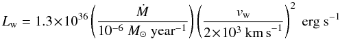 (3)where vw = 2000 km s-1 can be applied as the velocity of the stellar wind (Tielens 2005). Peng et al. (2010) found evidence for two expanding shells with a size of ~2.9 pc, comparable to the size of the extended high excitation region we have found. They found that a constant mass-loss rate of ~1.2 × 10⁻⁶ M⊙ yr-1 can sustain a wind-driven bubble with a size of ~2.9 pc, which corresponds to the mass loss rate of one O-type star. Using these values, the mechanical luminosity is Lw = 1.56 × 1036 erg s-1 or about 405 L⊙. Assuming an efficiency of 1 − 10% (Loenen et al. 2008), the mechanical heating rate is ~4−40.5 L⊙. However, this is only a lower limit of the luminosity corresponding to the mechanical heating. Alves & Homeier (2003) estimate that ~30 O-type stars belong to the central stellar cluster, which has a diameter of ~6 pc. Taking this into account, the mass-loss rate, as well as the luminosity is about an order of magnitude larger than the value we derive by taking a mass-loss rate that belongs to one O-type star. This gives 40.5 − 405 L⊙ as a mechanical heating luminosity.
In addition to the effect of stellar winds, protostellar outflows give a contribution to the mechanical heating. The largest outflow is connected to the most luminous water-maser emission in the Milky Way (Gwinn et al. 1992). It has been characterized by Scoville et al. (1986) and recently by Smith et al. (2009). Adopting an outflow dynamical time-scale of 104 yr, that corresponds to an average ~25 km s-1 outflow speed (Smith et al. 2009), an energy of 4.4 × 1047 erg (Scoville et al. 1986, scaled to a distance of 11.4 kpc), the mechanical luminosity is Lmech = 1.4 × 1036 erg s-1 or about ~400 L⊙. Assuming the same efficiency as for the mechanical luminosity produced by the stellar wind, only the most powerful outflow produces a mechanical luminosity that is 10% of the mechanical luminosity produced by the stellar winds of an embedded cluster of ~30 O-type stars. This estimate gives a lower limit on the mechanical luminosity produced by outflows. Additional kinetic energy injection may have been resulted by past outflows of the current O-type stars. These flows may still be dissipating energy. The existence of these flows may be probed using ALMA.
An additional source of the mechanical heating may exist in the form of shocks driven by the expansion of the (UC)Hii regions into the molecular cloud. The corresponding heating rate is proportional to the kinetic energy injection rate and is given by: 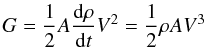 (4)where A is the surface area of the shocks, ρ is the density of the medium into which the shock is moving, and V is the velocity of the shock. The surface area of the shocks can be estimated based on De Pree et al. (1997), who measure the sizes of the (UC)Hii regions, based on high-resolution (0
 8) 3.6 cm data. We use an average radius of 0.05 pc to calculate the surface area of the shocks. Based on n(H2) = 106 cm-3, a shock velocity of 10 km s-1 results in a heating rate of 1.6 × 1037 erg s-1 for a cluster of 30 O-type stars. For a shock velocity of 5 km s-1, the mechanical heating rate of the expanding (UC)Hii regions corresponding to the cluster of 30 O-type stars is ~2 × 1036 erg s-1 – in the same order of magnitude as the mechanical heating produced by the stellar winds of the 30 O-type stars.
Radiative heating by the embedded stellar cluster.
The importance of heating by UV radiation from young massive stars, in the form of photo-electric emission by dust grains and PAHs, can be estimated from the far-infrared luminosity. Vastel et al. (2001) estimates a total FIR flux of 1.54 × 10⁻⁶ erg s-1 cm-2, which, at the distance of W49A, is equivalent to a total IR luminosity of 6.3 × 10⁶ L⊙. Adopting an efficiency of 10-3 − 10-2 (Meijerink & Spaans 2005), the heating rate by UV irradiation is on the same order of magnitude as the luminosity that can be expected from the mechanical heating.
X-ray heating.
Hard X-ray emission has been detected (Tsujimoto et al. 2006) toward the center of W49A, associated with two Hii regions. They measure an X-ray luminosity of 3 × 1033 erg s-1 in the 3−8 keV band. Assuming an efficiency of 10% (Meijerink & Spaans 2005), the X-ray heating luminosity is on the order of 0.1 L⊙, about three orders of magnitudes below the luminosity of the mechanical and UV heating. In addition, since X-ray emission is due to point-sources, rather than an extended region, X-rays mostly act locally and seem less likely to be responsible for the extended emission region what we detected.
Gas-grain collisional heating.
At the densities estimated using HCN transitions (105–106 cm-3), gas-grain collisions may give a significant contribution to the heating of the gas. Based on a greybody fit to the dust emission, Ward-Thompson & Robson (1990) derive a dust temperature of 50 K. They also find evidence, that a population of small, hot dust grains with T ~ 350 K also exists, based on an excess in the near-infrared. The heating rate of the gas per unit volume can be estimated using (Hollenbach & McKee 1979, 1989): ![Mathematical equation: \begin{eqnarray} \label{gasgrain} \Gamma_\mathrm{coll.}&=&1.2 \times 10^{-31}n^2 \left(\frac{T_{\rm{kin}}}{1000}\right)^{1/2} \left( \frac{100~\AA}{a_{\rm{min}}} \right)^{1/2} \\ && \times [1-0.8 \exp{(-75/T_{\rm{kin}}})] (T_{\rm{d}}-T_{\rm{kin}})~ \left(\mathrm{erg~cm^{-3}~s^{-1}}\right) \nonumber \end{eqnarray}](/articles/aa/full_html/2012/06/aa18582-11/aa18582-11-eq189.png) (5)where the minimum grain size is set at amin = 10 Å. Using T ~ 150 K and n = 106 cm-3, assuming a volume filling factor of 1–10% for the hot gas, a gas-to-dust ratio of 100, and that the fraction of the warm (T ~ 350 K) dust is up to 1% of the total dust, gas-grain heating for a 3 × 3 pc region toward the center of W49A is expected to be ~1034–1035 erg s-1, equivalent to ~3–30 L⊙.
(5)where the minimum grain size is set at amin = 10 Å. Using T ~ 150 K and n = 106 cm-3, assuming a volume filling factor of 1–10% for the hot gas, a gas-to-dust ratio of 100, and that the fraction of the warm (T ~ 350 K) dust is up to 1% of the total dust, gas-grain heating for a 3 × 3 pc region toward the center of W49A is expected to be ~1034–1035 erg s-1, equivalent to ~3–30 L⊙.
Based on these estimates, mechanical heating and UV heating seem to be the most probable heating mechanisms, while irradiation by X-rays and gas-grain collisions are less probable. The contribution of radiation to the excitation of W49A has been investigated earlier by Roberts et al. (2011), based on HCN, HNC and HCO+ transitions from the SLS. By comparing the observed line intensity ratios to PDR (Photon-dominated Region) and XDR (X-ray Dominated Region) models of Meijerink et al. (2007), they find, that HCN/HCO+ line ratios are consistent with PDR models, while HCN/HNC line ratios are consistent with XDR models. They interpret this result as evidence that irradiation by UV and X-ray photons plays a minor role in the excitation of W49A. However, as seen above, based on the UV heating luminosity, UV radiation cannot be ruled out to contribute significantly to the heating of W49A.
4.2. Comparison to the cooling rate
One of the main contributions to the total cooling in W49A is expected to occur via CO lines, therefore we derive a lower limit on the total cooling rate from the 12CO 3−2 (345.8 GHz) line luminosity based on data from the SLS. The CO line luminosity can be calculated from the CO 3−2 line intensities (Solomon & Vanden Bout 2005), as ![Mathematical equation: \begin{equation} \label{l_co} L_{\rm{CO}}\left[\!{\rm K\,km\,s^{-1}\,pc{^2}}\!\right]\!=\!23.5\Omega [{\rm{arcsec}}^2] (d [{\rm{Mpc}}])^2 I_{\rm{CO}} \left[\!{\rm{K\,km\,s^{-1}}}\!\right] \end{equation}](/articles/aa/full_html/2012/06/aa18582-11/aa18582-11-eq195.png) (6)or alternatively, in units of L⊙:
(6)or alternatively, in units of L⊙: ![Mathematical equation: \begin{equation} \label{l_co_lsun} L_{\rm{CO}}~[L_\odot]=1.04\,\times\,10^{-3} S_{\rm{CO}} [{\rm{Jy}}] \Delta {V} \left[{\rm{km\,s^{-1}}}\right] \nu [{\rm{GHz}}] (d [{\rm{Mpc}}])^2 \end{equation}](/articles/aa/full_html/2012/06/aa18582-11/aa18582-11-eq196.png) (7)where ICO = 593.4 K km s-1, TB = 34.5 K, SCO = 1.2 × 10⁴ Jy (using the Rayleigh-Jeans law to convert the brightness temperature to flux density) and ΔV = 17.2 km s-1 is the average line width. These numbers correspond to a spectrum smoothed to a FWHM = 1′ beam, which covers the high-excitation region around the center. Using these numbers, LCO(3−2) = 6.5 × 10³ K km s-1 pc2 = 9.65 L⊙ for the highly excited central square arcminute region. The fraction of the flux of the CO 3–2 transition to the total CO line flux can be estimated using Radex, adopting an H2 volume density of 106 cm-3 and a CO column density of 1019 cm-2. The CO column density estimate is based on the C17O 3−2 transition (at ~337 GHz) and a ratio of 16O/17O ~ 1800 (Wilson & Rood 1994). For Tkin = 100 K, the 3 − 2 transition is expected to be 9%, and for Tkin = 300 K, 5% of the total CO line flux. Using our Radex estimates of the total CO line flux:
(7)where ICO = 593.4 K km s-1, TB = 34.5 K, SCO = 1.2 × 10⁴ Jy (using the Rayleigh-Jeans law to convert the brightness temperature to flux density) and ΔV = 17.2 km s-1 is the average line width. These numbers correspond to a spectrum smoothed to a FWHM = 1′ beam, which covers the high-excitation region around the center. Using these numbers, LCO(3−2) = 6.5 × 10³ K km s-1 pc2 = 9.65 L⊙ for the highly excited central square arcminute region. The fraction of the flux of the CO 3–2 transition to the total CO line flux can be estimated using Radex, adopting an H2 volume density of 106 cm-3 and a CO column density of 1019 cm-2. The CO column density estimate is based on the C17O 3−2 transition (at ~337 GHz) and a ratio of 16O/17O ~ 1800 (Wilson & Rood 1994). For Tkin = 100 K, the 3 − 2 transition is expected to be 9%, and for Tkin = 300 K, 5% of the total CO line flux. Using our Radex estimates of the total CO line flux: 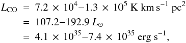 gives a lower limit on the cooling, with an accuracy of ~20%, mainly as a contribution from the typical calibration error in deriving the CO 3 − 2 line intensity.
Based on Neufeld et al. (2005), for kinetic temperatures >100 K and H2 volume densities ~106 cm-3, the total cooling is up to an order of magnitude above the CO cooling, ~103 L⊙.
Our estimates of the heating rate indicate that the two most important mechanisms to consider for W49A, are mechanical heating by the winds of O-type stars and UV-irradiation. These two mechanisms give a heating rate equivalent with 1000 L⊙, depending on the heating efficiency. This is of a same order of magnitude as the expected total cooling, assuming that the total cooling rate is a factor of 10 higher than the CO cooling rate. This result supports that the effect of embedded O-type stars in the form of stellar winds and UV-irradiation can explain the high-excitation region around the center of W49A.
4.3. Comparison to other warm and dense regions
Galactic center.
In our Galaxy, a similar level of excitation to what we found toward W49A was reported for clouds near the center. Hüttemeister et al. (1993) measured kinetic temperatures in 36 clouds near the Galactic center and based on NH3 transitions, they have found a temperature component of ~200 K, together with a cold gas and dust component. This sample, however, include no embedded stars, which could explain the highly excited gas component, and therefore, cannot be used as an analogue for W49A. De Vicente et al. (1997) have detected hot molecular gas toward the Sagittarius B2 molecular cloud. The highest temperatures measured toward Sagittarius B2 are in the range between 200 − 400 K, with typical densities of 106−107 cm-3, similar to what we find for the center of W49A. However, these conditions correspond to hot cores with sizes in the range of 0.5 − 0.7 pc, much smaller than the region with similar physical properties in W49A. De Vicente et al. (1997) have also found a more extended component of warm (100 − 120 K) gas as a ring surrounding Sgr B2M and Sgr B2N with a radius of 2 pc and a thickness of 1.4 pc, with a density of about 2 × 105 cm-3. Ferrière et al. (2007) study physical conditions in the innermost 3 kpc of the Galaxy, and find a high-temperature gas component (T ~ 150 K), however, it corresponds to a low-density environment (nH2 ~ 102.5 cm-3), unlike what we find for W49A. On Galactic scales, W49A shows a uniquely extended region of high (T ≳ 100 K) temperature which appears to be tracing the feedback from the young and forming stars in the region on their surrounding gas.
Starbursts and active galaxies.
In even nearby galaxies sensitivity and angular resolution mean that the physical conditions of the molecular gas can only be estimated on ~100 pc scales with uncertain filling factors. Nevertheless there are regions where temperatures similar to those in W49A are measured. In particular, extended warm molecular gas ( > 100 K) has been detected in a number of starburst- and Seyfert galaxies (e.g. Rigopoulou et al. 2002). Mühle et al. (2007) have detected a warm, Tkin ~ 200 K gas component with moderate density (n(H2) = 7 × 103 cm-3) in the starburst galaxy M82, using p-H2CO line ratios, probing scales of ~320 pc. Ott et al. (2005) derived kinetic temperatures of 140 K and 200 K toward two positions of the starburst galaxy NGC 253, using NH3(3, 3) ATCA data on a scale of 65 pc. Mauersberger et al. (2003) have detected a warm (100 − 140 K) gas component toward the center of three nearby starburst galaxies (NGC 253, IC 342 and Maffei 2) for regions of 300 − 660 pc, based on NH3 (1, 1)–(6, 6) transitions. An even warmer component (T > 400 K) was detected toward IC 342. Papadopoulos et al. (2012), based on a sample of 70 (Ultra-)Luminous Infrared Galaxies, most of them dominated by a warm (Tkin > 100 K) and dense (n > 104 cm-3) gas phase with masses of ~109 M⊙, come to the conclusion that the main heating mechanism is rather cosmic-rays and highly supersonic turbulence than far-UV radiation or shocks related to star-formation. This might be one of the key differences between the extended, but compared to scales of entire galaxies, still local phenomenon seen for W49A, and starburst galaxies. However, in the context of the Milky Way, W49A is a close analogue in terms of physical parameters to regions in starburst- and active galaxies.
Another key comparison with warm (≳100 K) and dense (≳105 cm-3) regions, such as starburst galaxies, is the initial mass function (IMF). Klessen et al. (2007) have found, based on hydrodynamical numerical calculations, that for regions of warm (~100 K) and dense (≳105 cm-3) gas, the slope of the IMF is in the range of − 1.0 and − 1.3, with a turn-over mass of 7 M⊙. Homeier & Alves (2005) derived an IMF in W49A with a slope of −1.70 ± 0.30 and −1.6 ± 0.3 down to masses of ~10 M⊙. This result may be consistent with the calculations of Klessen et al. (2007), and if so, supports that W49A is a Galactic template for starburst galaxies. However, incompleteness at low luminosities and masses might explain the observed cut-off at masses of ~10 M⊙.
Pressure as a diagnostic of starburst environments.
Environments with increased star-formation activity, such as starburst galaxies, massive star-forming regions and clouds near the Galactic center can be characterized with their pressures, P/k ~ nT. Typical pressures that can be expected in the Galaxy and in the midplane of ordinary spirals are in the order of 104 K cm-3 (Papadopoulos et al. 2012). Table 4 shows the measured values of n, T and P/k for W49A, Sgr B2 and starburst galaxies. P/k values show more than an order of magnitude variation. Based on our derived densities and temperatures, the gas pressure in W49A is up to 5.4 × 10⁸ K cm-3, similar to those measured toward SgrB2 and Arp 220. Other galactic nuclei appear to have lower pressures, which seems to be mainly the effect of a lower gas density. Beam dilution seems not to play a major effect for the density estimates, given the high densities measured toward Arp 220 as well as the sensitivity, which makes measurements in external galaxies biased toward the warm and dense gas. However, the estimated densities significantly depend on the tracer used, as was shown by Greve et al. (2009), who find a 10−100 factor difference between densities estimated from HCN compared to densities estimated from HCO+. Therefore, the uncertainty in P/k is about an order of magnitude.
Pressures measured toward W49A and Sgr B2 are not entirely unique in our Galaxy. Dense gas has been detected toward a number of massive star forming regions, such as reported by Plume et al. (1997), Wu et al. (2010) and McCauley et al. (2011). However, the temperatures of those regions are only comparable to what we measure toward W49A “locally”, on sub-parsec scales, corresponding to hot cores, such as toward Orion KL (Mangum & Wootten 1993). Considering the spatial extent, pressures measured toward W49A provide a Galactic analogue of starburst galaxies.
Comparison of physical parameters in W49A to Galactic center clouds and starburst galaxies.
5. Summary and conclusions
We have analyzed the physical conditions towards the central 2 × 2 arcminutes region of W49A using JCMT maps with 15′′ resolution. We have reported a detection of warm (>100 K) and dense (>105 cm-3) gas toward the center, extending up to a few parsecs.
-
We have characterized the excitation toward four main regions of W49A (center, northern clump, southwest clump and eastern tail) based on rotational diagrams of SO2, CH3 OH and H2 CO, taking into account the optical depth and beam dilution. High excitation and column densities, as well as significant beam dilution is seen towards the center, likely to trace embedded hot cores. The off-center positions show excitation temperatures corresponding to about half of those derived for the center, and no significant beam dilution.
-
Based on o-H2CO line ratios, we estimate kinetic temperatures of the main regions of W49A. Toward the center, we derive a kinetic temperature of 250−300 K, 60−100 K toward the northern clump, 80−150 K toward the southwest clump and 70−130 K toward the eastern tail. Our estimates show an approximately 1′ × 1′ (~3.3 × 3.3 pc) region with extended warm (>100 K) gas towards the center of W49A. Based on HCN 3−2 / HCN 4−3 line ratios, the high-temperature central 1′ × 1′ region has H2 volume densities of > 105 cm-3. The high excitation of W49A is comparable to clouds near the center of our Galaxy and to starburst galaxies with estimates on scales of ~100 pc.
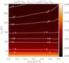
Fig. A.1 Line ratios of o-H2CO 515 − 414 and 533 − 432 as a function of kinetic temperature and H2 density for FWHM = 12 km s-1. The intensity scale is logarithmic.
-
The most important heating mechanisms for W49A are mechanical heating due to stellar winds of embedded, O-type stars and UV irradiation. X-ray irradiation and gas-grain collisional heating are less probable than other two mechanisms, while the effect of cosmic-rays remains an open question. However, the two main mechanisms corresponding to embedded young stellar populations provide a heating that no other mechanism is needed to contribute significantly in the heating of W49A. Based on earlier studies of starburst galaxies and their proposed heating mechanisms, W49A is a Galactic starburst analogue, in terms of excitation and physical conditions, but not in terms of the heating mechanism which yields the high excitation, due to additional heating mechanisms that have been proposed to explain the excitation of starburst- and active galaxies (such as cosmic rays or supersonic turbulence). Our future work includes an analysis of the chemical inventory as well as kinematics of selected species, based on the entire SLS survey including data from the main survey (330−360 GHz,Plume et al. 2007) and will be presented in Nagy et al. (in prep.).
The James Clerk Maxwell Telescope is operated by the Joint Astronomy Centre on behalf of the Science and Technology Facilities Council of the United Kingdom, The Netherlands Organisation for Scientific Research, and the National Research Council of Canada.
Acknowledgments
We thank the referees John Bally and Adam Ginsburg for the careful reading of the manuscript and for the constructive suggestions. We also thank the editor Malcolm Walmsley for additional helpful comments. The authors thank Alexandre Faure for discussion on H2CO collision rates, Kuo-Song Wang for advice about population diagrams and Paul Goldsmith for discussion about the cooling rates and volume filling factors. Z.N. acknowledges Stefanie Mühle and Chris dePree for their useful comments. We acknowledge the use of the CDMS and JPL databases for the rest frequencies.
References
- Aloisi, A., Tosi, M., & Greggio, L. 1999, ApJ, 118, 302 [Google Scholar]
- Alves, J., & Homeier, N. 2003, ApJ, 589, L45 [NASA ADS] [CrossRef] [Google Scholar]
- Bayet, E., Gerin, M., Phillips, T. G., & Contursi, A. 2004, A&A, 427, 45 [NASA ADS] [CrossRef] [EDP Sciences] [Google Scholar]
- Bradford, C. M., Nikola, T., Stacey, G. J., et al. 2003, ApJ, 586, 891 [NASA ADS] [CrossRef] [Google Scholar]
- Brogan, C. L., & Troland, T. H. 2001, ApJ, 550, 799 [NASA ADS] [CrossRef] [Google Scholar]
- Buckle, J. V., Hills, R. E., Smith, H., et al. 2009, MNRAS, 399, 1026 [NASA ADS] [CrossRef] [Google Scholar]
- Buckley, H. D., & Ward-Thompson, D. 1996, MNRAS, 281, 294 [NASA ADS] [Google Scholar]
- De Pree, C. G., Mehringer, D. M., & Goss, W. M. 1997, ApJ, 482, 307 [NASA ADS] [CrossRef] [Google Scholar]
- De Pree, C. G., Wilner, D. J., Mercer, A. J., et al. 2004, ApJ, 600, 286 [NASA ADS] [CrossRef] [Google Scholar]
- De Vicente, P., Martín-Pintado, J., & Wilson, T. L. 1997, A&A, 320, 957 [NASA ADS] [Google Scholar]
- Dumouchel, F., Faure, A., & Lique, F. 2010, MNRAS, 406, 2488 [NASA ADS] [CrossRef] [Google Scholar]
- Ferrière, K., Gillard, W., & Jean, P. 2007, A&A, 467, 611 [Google Scholar]
- Genzel, R., Downes, D., Moran, J. M., et al. 1978, A&A, 66, 13 [NASA ADS] [Google Scholar]
- Goldsmith, P. F., & Langer, W. D. 1999, ApJ, 517, 209 [NASA ADS] [CrossRef] [Google Scholar]
- Green, S. 1991, ApJS, 76, 979 [NASA ADS] [CrossRef] [Google Scholar]
- Greve, T. R., Papadopoulos, P. P., Gao, Y., & Radford, S. J. E. 2009, ApJ, 692, 1432 [NASA ADS] [CrossRef] [Google Scholar]
- Gwinn, C. R., Moran, J. M., & Reid, M. J. 1992, ApJ, 393, 149 [NASA ADS] [CrossRef] [Google Scholar]
- Homeier, N., & Alves, J. 2005, A&A, 430, 481 [NASA ADS] [CrossRef] [EDP Sciences] [Google Scholar]
- Hüttemeister, S., Wilson, T. L., Bania, T. M., & Martín-Pintado, J. 1993, A&A, 280, 255 [NASA ADS] [Google Scholar]
- Jaffe, D. T., Harris, A. I., & Genzel, R. 1987, ApJ, 316, 231 [NASA ADS] [CrossRef] [Google Scholar]
- Klessen, R. S., Spaans, M., & Jappsen, A.-K. 2007, MNRAS, 374, L29 [NASA ADS] [CrossRef] [Google Scholar]
- Loenen, A. F., Spaans, M., Baan, W. A., & Meijerink, R. 2008, A&A, 488, 5 [Google Scholar]
- Mangum, J. G., & Wootten, A. 1993, ApJS, 89, 123 [NASA ADS] [CrossRef] [Google Scholar]
- Mauersberger, R., Henkel, C., Weiß, A., Peck, A. B., & Hagiwara, Y. 2003, A&A, 403, 561 [NASA ADS] [CrossRef] [EDP Sciences] [Google Scholar]
- McCauley, P. I., Mangum, J. G., & Wootten, A. 2011, ApJ, 742, 58 [NASA ADS] [CrossRef] [Google Scholar]
- Meijerink, R., & Spaans, M. 2005, A&A, 436, 397 [NASA ADS] [CrossRef] [EDP Sciences] [Google Scholar]
- Meijerink, R., Spaans, M., & Israel, F. P. 2007, A&A, 461, 793 [NASA ADS] [CrossRef] [EDP Sciences] [Google Scholar]
- Mufson, S. L., & Liszt, H. S. 1977, ApJ, 212, 664 [NASA ADS] [CrossRef] [Google Scholar]
- Mundy, L. G., Evans, N. J., II, Snell, R. L., Goldsmith, P. F., & Bally, J. 1986, ApJ, 306, 670 [NASA ADS] [CrossRef] [Google Scholar]
- Mühle, S., Seaquist, E. R., & Henkel, C. 2007, ApJ, 671, 1579 [NASA ADS] [CrossRef] [Google Scholar]
- Naylor, B. J., Bradford, C. M., Aguirre, J. E., et al. 2010, ApJ, 722, 668 [NASA ADS] [CrossRef] [Google Scholar]
- Neufeld, D. A., Lepp, S., & Melnick, G. J. 1995, ApJS, 100, 132 [NASA ADS] [CrossRef] [Google Scholar]
- Ott, J., Weiß, A., Henkel, C., & Walter, F. 2005, ApJ, 629, 767 [NASA ADS] [CrossRef] [Google Scholar]
- Papadopoulos, P. P., van der Werf, P. P., Xilouris, E. M., et al. 2012, MNRAS, in press [arXiv:1109.4176] [Google Scholar]
- Peng, T., Wyrowski, F., van der Tak, F. F. S., Menten, K. M., & Walmsley, C. M. 2010, A&A, 520, A84 [NASA ADS] [CrossRef] [EDP Sciences] [Google Scholar]
- Plume, R., Jaffe, D. T., Evans, N. J., II,Martin-Pintado, J., & Gomez-Gonzalez, J. 1997, ApJ, 476, 730 [NASA ADS] [CrossRef] [Google Scholar]
- Plume, R., Fuller, G. A., Helmich, F., et al. 2007, PASP, 119, 102 [NASA ADS] [CrossRef] [Google Scholar]
- Rigopoulou, D., Kunze, D., Lutz, D., Genzel, R., & Moorwood, A. F. M. 2002, A&A, 389, 374 [NASA ADS] [CrossRef] [EDP Sciences] [Google Scholar]
- Roberts, H., Van der Tak, F. F. S., Fuller, G. A., Plume, R., & Bayet, E. 2011, A&A, 525, 107 [Google Scholar]
- Scoville, N. Z., Sargent, A. I., Sanders, D. B., et al. 1986, ApJ, 303, 416 [NASA ADS] [CrossRef] [Google Scholar]
- Serabyn, E., Guesten, R., & Schulz, A. 1993, ApJ, 413, 571 [NASA ADS] [CrossRef] [Google Scholar]
- Schöier, F. L., van der Tak, F. F. S., van Dishoeck, E. F., & Black, J. H. 2005, A&A, 432, 369 [NASA ADS] [CrossRef] [EDP Sciences] [Google Scholar]
- Sievers, A. W., Mezger, P. G., Bordeon, M. A., et al. 1991, A&A, 251, 231 [NASA ADS] [Google Scholar]
- Smith, N., Whitney, B. A., Conti, P. S., De Pree, C. G., & Jackson, J. M. 2009, MNRAS, 399, 952 [NASA ADS] [CrossRef] [Google Scholar]
- Snell, R. L., Goldsmith, P. F., Erickson, N. R., Mundy, L. G., & Evans, N. J., II. 1984, ApJ, 276, 625 [NASA ADS] [CrossRef] [Google Scholar]
- Solomon, P. M., & Van den Bout, P. A. 2005, ARA&A, 43, 677 [NASA ADS] [CrossRef] [Google Scholar]
- Tielens, A. G. G. M. 2005, The Physics and Chemistry of the Interstellar Medium, 1st edn. (Cambridge: Cambridge Univ. Press) [Google Scholar]
- Troscompt, N., Faure, A., Wiesenfeld, L., Ceccarelli, C., & Valiron, P. 2009, A&A, 493, 687 [NASA ADS] [CrossRef] [EDP Sciences] [Google Scholar]
- Tsujimoto, M., Hosokawa, T., Feigelson, E. D., Getman, K. V., & Broos, P. S. 2006, ApJ, 653, 409 [NASA ADS] [CrossRef] [Google Scholar]
- Turner, B. E. 1991, ApJS, 76, 617 [NASA ADS] [CrossRef] [Google Scholar]
- Van der Tak, F. F. S., Van Dishoeck, E. F., & Caselli, P. 2000, A&A, 361, 327 [NASA ADS] [Google Scholar]
- Van der Tak, F. F. S., Black, J. H., Schöier, F. L., Jansen, D. J., & van Dishoeck, E. F. 2007, A&A, 468, 627 [NASA ADS] [CrossRef] [EDP Sciences] [Google Scholar]
- Vastel, C., Spaans, M., Ceccarelli, C., Tielens, A. G. G. M., & Caux, E. 2001, A&A, 376, 1064 [NASA ADS] [CrossRef] [EDP Sciences] [Google Scholar]
- Ward-Thompson, D., & Robson, E. I. 1990, MNRAS, 244, 458 [NASA ADS] [Google Scholar]
- Welch, W. J., Dreher, J. W., Jackson, J. M., Terebey, S., & Vogel, S. N. 1987, Science, 238, 1550 [NASA ADS] [CrossRef] [PubMed] [Google Scholar]
- Williams, J. A., Dickel, H. R., & Auer, L. H. 2004, ApJS, 153, 463 [NASA ADS] [CrossRef] [Google Scholar]
- Wilner, D. J., De Pree, C. G., Welch, W. J., & Goss, W. M. 2001, ApJ, 550, L81 [NASA ADS] [CrossRef] [Google Scholar]
- Wilson, T. L., & Rood, R. 1994, ARA&A, 32, 191 [NASA ADS] [CrossRef] [Google Scholar]
- Wu, J., Evans, N. J., II, Shirley, Y. L., & Knez, C. 2010, ApJS, 188, 313 [NASA ADS] [CrossRef] [Google Scholar]
- Zhu, M., Seaquist, E. R., & Kuno, N. 2003, ApJ, 588, 243 [NASA ADS] [CrossRef] [Google Scholar]
Appendix A: Radex line ratio plots
In Sects. 3.3 and 3.4 we compare the observed line ratios to line ratios calculated using the non-LTE code Radex (Van der Tak et al. 2007). Figure A.1 shows the the o − H2CO 515−414 and 533 − 432 line intensity ratios for H2 volume densities between 103 cm-3 and 106 cm-3 and temperatures between 20 K and 300 K. Figure A.2 shows the HCN 3−2 and 4−3 line intensity ratios for H2 column densities between 103 cm-3 and 108 cm-3 and temperatures between 20 K and 300 K. Both of these calculations use a molecular column density of 1014 cm-2 and a background temperature of 2.73 K. We assume a line width of FWHM = 12 km s-1 for H2CO , and a line width of 18 km s-1 for HCN for the central 40′′ × 40′′, in consistence with the observed line widths.
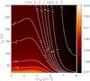 |
Fig. A.2 Line ratios of HCN 3−2 and 4−3 as a function of kinetic temperature and H2 density for FWHM = 18 km s-1. |
All Tables
Comparison of physical parameters in W49A to Galactic center clouds and starburst galaxies.
All Figures
|
Fig. 1 The spectrum towards the source center (RA(J2000) = 19:10:13.4; Dec(J2000) = 09:06:14) in the 360−373 GHz frequency range of the SLS. The main detected lines are labeled. The gap in the spectrum around 368.5 GHz is a region of high atmospheric extinction and was not observed. |
| In the text | |
|
Fig. 2 The integrated intensity distribution of HCN 4−3, SO2 152,14−141,13, CH3OH 72,5−61,5 and H2CO 515−414. The central position is shown with black plus signs, the off-center regions (northern clump, eastern tail and southwest clump) are also shown with white plus signs. |
| In the text | |
|
Fig. 3 The results of the rotation diagram analysis for H2CO toward the center. Top panels: the results of the rotation diagram analysis before (red symbols) and after (green symbols) corrections for optical depth and beam dilution. The overplotted blue line corresponds to a linear fit to the rotational diagram without corrections. Bottom panels: the corresponding best fit optical depths from the χ2 minimization. |
| In the text | |
|
Fig. 4 The results of the rotation diagram analysis for H2CO at off-center positions. Top panels: the results of the rotation diagram analysis before (red symbols) and after (green symbols) corrections for optical depth and beam dilution. The overplotted blue line corresponds to a linear fit to the rotational diagram without corrections. Bottom panels: the corresponding best fit optical depths from the χ2 minimization. |
| In the text | |
|
Fig. 5 Left panel: ratio of 533−432 to the 515−414 H2CO transition. Right panel: kinetic temperature map of W49A determined from line ratio shown in the left panel. |
| In the text | |
|
Fig. 6 Map of the line ratio of HCN J = 4 − 3 to HCN J = 3 − 2. |
| In the text | |
|
Fig. 7 Volume density estimates from the HCN 3 − 2 and HCN 4 − 3 lines. |
| In the text | |
|
Fig. A.1 Line ratios of o-H2CO 515 − 414 and 533 − 432 as a function of kinetic temperature and H2 density for FWHM = 12 km s-1. The intensity scale is logarithmic. |
| In the text | |
|
Fig. A.2 Line ratios of HCN 3−2 and 4−3 as a function of kinetic temperature and H2 density for FWHM = 18 km s-1. |
| In the text | |
Current usage metrics show cumulative count of Article Views (full-text article views including HTML views, PDF and ePub downloads, according to the available data) and Abstracts Views on Vision4Press platform.
Data correspond to usage on the plateform after 2015. The current usage metrics is available 48-96 hours after online publication and is updated daily on week days.
Initial download of the metrics may take a while.