| Issue |
A&A
Volume 541, May 2012
|
|
|---|---|---|
| Article Number | A73 | |
| Number of page(s) | 10 | |
| Section | Interstellar and circumstellar matter | |
| DOI | https://doi.org/10.1051/0004-6361/201118575 | |
| Published online | 01 May 2012 | |
Multi-line detection of O2 toward ρ Ophiuchi A⋆
1 Department of Earth and Space SciencesChalmers University of Technology, Onsala Space Observatory, 439 92 Onsala, Sweden
e-mail: This email address is being protected from spambots. You need JavaScript enabled to view it.
2 Jet Propulsion Laboratory, California Institute of Technology, 4800 Oak Grove Drive, Pasadena CA 91109, USA
3 Department of Astronomy, Stockholm University, 106 91 Stockholm, Sweden
4 LERMA & UMR 8112 du CNRS, Observatoire de Paris, 61 Av. de l’Observatoire, 75014 Paris, France
5 Onsala Space Observatory, Chalmers University of Technology, 439 92 Onsala, Sweden
6 Observatoire de Paris, LUTH, Paris, France
7 Centro de Astrobiología, CSICINTA, 28850 Madrid, Spain
8 Institute of Astronomy, ETH-Zurich, Zurich, Switzerland
9 Department of Astronomy, University of Michigan, 500 Church Street, Ann Arbor MI 48109, USA
10 School of Physics and Astronomy, University of Leeds, Leeds, UK
11 Université de Toulouse, UPS-OMP, IRAP, Toulouse, France & CNRS, IRAP, 9 Av. Colonel Roche, BP 44346, 31028 Toulouse Cedex 4, France
12 LRA/LERMA, CNRS, UMR8112, Observatoire de Paris & École Normale Supérieure, 24 rue Lhomond, 75231 Paris Cedex 05, France
13 SETI Institute, Mountain View CA 94043, USA
14 Department of Physics and Astronomy, San José State University, San Jose CA 95192, USA
15 National Astronomical Observatories, Chinese Academy of Sciences, A20 Datun Road, Chaoyang District, 100012 Beijing, PR China
16 California Institute of Technology, Cahill Center for Astronomy and Astrophysics 301-17, 1200 E. California Boulevard, Pasadena CA 91125, USA
17 Harvard-Smithsonian Center for Astrophysics, 60 Garden Street, MS 66, Cambridge MA 02138, USA
18 SRON Netherlands Institute for Space Research, PO Box 800, 9700 AV,
and Kapteyn Astronomical Institute, University of Groningen, Groningen, The Netherlands
19 Department of Astronomy, University of Massachusetts, Amherst MA 01003, USA
20 Leiden Observatory, Leiden University, PO Box 9513, 2300 RA Leiden, The Netherlands
21 Max-Planck-Institut für Extraterrestrische Physik, Gießenbachstraße 1, 85748 Garching, Germany
22 Department of Physics and Astronomy, University College London, London, UK
Received: 4 December 2011
Accepted: 7 March 2012
Abstract
Context. Models of pure gas-phase chemistry in well-shielded regions of molecular clouds predict relatively high levels of molecular oxygen, O2, and water, H2O. These high abundances imply high cooling rates, leading to relatively short timescales for the evolution of gravitationally unstable dense cores, forming stars and planets. Contrary to expectations, the dedicated space missions SWAS and Odin typically found only very small amounts of water vapour and essentially no O2 in the dense star-forming interstellar medium.
Aims. Only toward ρ Oph A did Odin detect a very weak line of O2 at 119 GHz in a beam of size 10 arcmin. The line emission of related molecules changes on angular scales of the order of some tens of arcseconds, requiring a larger telescope aperture such as that of the Herschel Space Observatory to resolve the O2 emission and pinpoint its origin.
Methods. We use the Heterodyne Instrument for the Far Infrared (HIFI) aboard Herschel to obtain high resolution O2 spectra toward selected positions in the ρ Oph A core. These data are analysed using standard techniques for O2 excitation and compared to recent PDR-like chemical cloud models.
Results. The NJ = 33 − 12 line at 487.2 GHz is clearly detected toward all three observed positions in the ρ Oph A core. In addition, an oversampled map of the 54−34 transition at 773.8 GHz reveals the detection of the line in only half of the observed area. On the basis of their ratios, the temperature of the O2 emitting gas appears to vary quite substantially, with warm gas ( ≳ 50 K) being adjacent to a much colder region, of temperatures lower than 30 K.
Conclusions. The exploited models predict that the O2 column densities are sensitive to the prevailing dust temperatures, but rather insensitive to the temperatures of the gas. In agreement with these models, the observationally determined O2 column densities do not seem to depend strongly on the derived gas temperatures, but fall into the range N(O2) = 3 to ≳ 6 × 1015 cm-2. Beam-averaged O2 abundances are about 5 × 10⁻⁸ relative to H2. Combining the HIFI data with earlier Odin observations yields a source size at 119 GHz in the range of 4 to 5 arcmin, encompassing the entire ρ Oph A core. We speculate that one of the reasons for the generally very low detection rate of O2 is the short period of time during which O2 molecules are reasonably abundant in molecular clouds.
Key words: ISM: abundances / ISM: molecules / ISM: lines and bands / ISM: clouds / ISM: individual objects:ρOph A SM 1 / stars: formation
Based on observations with Herschel-HIFI. Herschel is an ESA space observatory with science instruments provided by European-led Principal Investigator consortia and with important participation from NASA.
© ESO, 2012
1. Introduction
Despite the universal importance of oxygen, its molecular form, O2, is an elusive species of the interstellar medium (ISM). This molecule was thought to be one of the main regulators of the energy balance in the ISM, as summarised by Goldsmith & Langer (1978). Consequently, large efforts, from both the ground (O18O) and space, were made to obtain quantitative estimates of its abundance. The historical account of this essentially fruitless “O2-struggle” was reviewed by Goldsmith et al. (2011). Prior to Herschel, both SWAS (Melnick et al. 2000; Goldsmith et al. 2000) and Odin (Nordh et al. 2003; Pagani et al. 2003) had already shown that the abundances of both O2 and H2O assumed by Goldsmith & Langer (1978) were much higher than actual values in the ISM and, with the exception of the ρ Oph cloud, none of the O2 lines were detected anywhere in the ISM. Goldsmith et al. (2002) announced the tentative detection by SWAS of the O2 487 GHz line in ρ Oph A. The claimed signal appeared at an unusual velocity and was atypically broad. Pagani et al. (2003) showed that, based on more sensitive O2 119 GHz observations with Odin, this was an erroneous result. This line was finally detected by Odin, at the correct local standard of rest (LSR) velocity and with a plausible, narrow line-width (Larsson et al. 2007). Here we report the detection of two more O2 transitions in ρ Oph A, viz. at 487 GHz and at 774 GHz, respectively.
Instrumental reference.
Source designations and coordinates for ρ Oph A, with positions observed in O2 in bold face.
Besides being relatively nearby (120 − 130 pc, Lombardi et al. 2008; Snow et al. 2008; Mamajek 2008; Loinard et al. 2008), the ρ Oph cloud distinguishes itself from other low-mass star-forming regions in that it exhibits evidence (e.g., in C18O line emission) of gas at relatively high temperatures (T ≥ 20 K) over extended regions with high column densities (N(H2) ≫ 1022 cm-2, Liseau et al. 2010). In addition, ρ Oph A displays an interesting chemistry: doubly deuterated formaldehyde (D2CO) and hydrogen peroxide (H2O2) molecules, rarely seen elsewhere in the ISM, have for example been found here (Bergman et al. 2011a,b). The overall impression is that the observable abundance of many species is the result of surface reactions on dust grains, a process that may also pertain to the production of oxygen molecules.
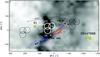 |
Fig. 1 Herschel beams of O2 487 GHz (44′′) superposed onto a grey scale C18O (3 − 2) map of ρ Oph A (Liseau et al. 2010). The + and × symbols designate the positions of the H- and V-polarization beam centres of HIFI, respectively, with a separation of 6 |


The first motivation behind our Herschel observations was to pin down the precise location of the O2 source inside the large, ten-arcminute beam of Odin. Secondly, we wished to add observations of the O2 487.25 GHz (33 − 12) and 773.84 GHz (54 − 34) lines, which have upper level energies Eup/k = 26 K and 61 K, respectively, to the Odin data of the 118.75 GHz (11 − 10) transition (Eup/k = 6 K). These observations should enable us to learn something about the nature of the O2 source in the ρ Oph cloud. This could then be compared to the physical and chemical conditions of other locations in the general ISM and potentially identify the characteristics and timescales of regions containing O2 molecules.
The paper is organised as follows: in Sect. 2, our Herschel-HIFI observations and their reduction are discussed in considerable detail and our results are presented in Sect. 3. These results are discussed in Sect. 4, where the spectral line formation is analysed under different assumptions. Finally, in Sect. 5, our main conclusions are briefly summarised.
2. Observations and data reduction
Herschel is a space platform for far-infrared and sub-millimetre observations (Pilbratt et al. 2010). It orbits the Sun about 1.5 million kilometres beyond the Earth (at L 2) and its 3.5 m primary dish is radiatively cooled to its operational equilibrium temperature of about 85 K. The scientific instruments are placed in a liquid-helium-filled cryostat, limiting its cold lifetime to roughly 3.5 years. One of the three onboard instruments is the Heterodyne Instrument for the Far Infrared (HIFI, De Graauw et al. 2010) with continuous frequency coverage from 480 GHz to 1250 GHz (λλ 624 − 234 μm) in 5 bands. In addition, the frequency range 1410 GHz to 1910 GHz (λλ 213 − 157 μm) is covered by bands 6 and 7. The spectral resolving capability is the highest available on Herschel, i.e. up to 107 corresponding to 30 m s-1, and is required to resolve the profiles of very narrow lines of cold sources, which have temperatures of the order of 10 K or less.
Spectral line data and the relevant characteristics of the instruments discussed in this paper have been compiled in Table 1.
2.1. The 487 GHz observations
The 487 GHz observations with HIFI were performed on operating day OD 673 (2011 March 18). The three positions O1, O3, and O4 at the centre of the ρ Oph A core (Table 2) were observed in double beam-switch mode (DBS), with beam throws of 3′ in roughly the west and east directions (with a position angle of 101° E of N) and identified in Fig. 1 by the numbers 6031 and 6032, respectively. For each position, the relative observing time spent on the east- and westward on-off pairs was 7.3 h, and the total programme execution time was 21.9 h. The DBS mode generally produces the highest quality data with HIFI and since the O2 signal is known to be weak, this was the observing mode chosen. Switching by only three arcminutes inside a molecular cloud is generally considered not to be a sensible option, as this potentially results in the cancellation of the source signal. However, a relatively large velocity gradient (≳0.3 km s-1/arcmin) and/or two distinctly different velocity systems (Δυ ~ 1 km s-1) are known to exist in ρ Oph A (e.g., Bergman et al. 2011a). In addition, the O2 line is known to be narrow (FWHM ~ 1 km s-1). Hence, all of these factors taken together suggest that the risk of signal cancellation is low. Splitting the entire data set into two and reducing these two halves with only one of the off-spectrua used resulted in essentially the same spectral data. These off-beams were pointed at very different regions in ρ Oph A (Fig. 1), but no traceable off-beam contamination was introduced by the DBS observations.
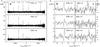 |
Fig. 2 Average double side band (DSB) spectra of H- and V-polarizations for the three positions O1, O3, and O4 in the ρ Oph A cloud core, shown for the range 484.65 GHz to 489.85 GHz. The spectral lines are found exclusively in the lower side band (LSB) and the LSR velocity, υLSR, along the abcissa is in km s-1 and the antenna temperature TA along the ordinate in mK. a) 5 GHz wide band of the WBS around the 487 O2 line ( − 1600, + 1600 km s-1). b) The WBS spectrum at expanded scale, showing the O2 line at 487 GHz, which is detected in all three positions. Inspection of the individual on-off pairs suggests that the apparent absorption features next to the lines are not real but simply due to the noise. c) Similar to b) but for the corresponding HRS data. |
O2 line observations of ρ Oph A.
The receivers are double side-band and to counteract confusion in frequency space, we selected for each observation 8 different LO-tunings inside HIFI-band 1a, spaced by 170 MHz to 260 MHz. During data reduction, this allowed us to perform a sideband deconvolution and identify any “false” signal due to a strong feature in the other sideband, which might otherwise have been folded over onto the weak O2 feature.
We used both the Wide Band Spectrometer (WBS) and the High Resolution Spectrometer (HRS) with respective resolutions 1.10 MHz and 250 kHz (0.68 and 0.15 km s-1). The positions of spikes and spectrometer artifacts are known and flagged, and none of these interfered with the O2 observations. Initial data reduction and calibrations were performed with the standard Herschel pipeline HIPE version 7.1 and the subsequent data analysis was made with a variety of other software packages. The quality of the HIFI data is excellent and it was sufficient to subtract a low-order baseline for each LO setting prior to averaging. The intensity calibration accuracy is estimated to be 10%.
The frequency-dependent beam widths (HPBW) and main beam efficiencies (ηmb) were adopted from Roelfsema et al. (2012). Before averaging the data for a given position, the H- and V-polarization spectra were all inspected individually in order to avoid the suppression of weak spectral lines or the generation of artificial features.
2.2. 774 GHz observations
The 774 GHz observations with HIFI band 2 were made on OD 583 (2011 September 15). A 6 × 6 map, aligned with the equatorial celestial coordinates (Fig. 3), was obtained with a 10′′ regular spacing, oversampling the 28′′ beam by nearly a factor of three and allowing for potentially increased spatial information of the emission regions.
Both the WBS (0.43 km s-1) and the HRS (0.097 km s-1) were used. The 774 GHz data were also obtained in DBS mode, with the offset positions displaced by 3′ and in nearly the same chopping direction as before (along PA = 98°). With 500 s on-source integrations at each position, the total observing time was 12 h.
3. Results
In the figures showing HIFI data, brightness is given as the antenna temperture, TA. When more than one telescope had been used, the data are presented on the main beam brightness temperature scale, Tmb, where the main-beam efficiency is ηmb = 0.75 for both HIFI transitions (Roelfsema et al. 2012) and 0.9 for the Odin transition (Frisk et al. 2003; Hjalmarson et al. 2003) and where we use the relation TA/ηmb = Tmb. For completeness, we also provide in Table 3, together with the HIFI data, the results of the Odin observations.
3.1. 487 GHz
The reduced WBS spectra for the three positions O1, O3, and O4 are shown for the frequency range 484.65 GHz to 489.85 GHz in Fig. 2a. The upper side band (USB) is completely line-free, i.e. all line detections refer to the LSB only. The presented data are DSB in order to suppress the noise. Centred on the O2 line, radial velocities span − 1600 to +1600 km s-1. In addition to the detected O2 487.25 GHz lines near an LSR velocity of 3 km s-1 in all three positions, the spectra show a number of other emission features that correspond to identified molecular lines, of, e.g., CS, CH3OH, NH2D, and SO, to mention only the strongest ones. In addition these spectra reveal variations in intensity and line width on angular scales of only some tens of arcsec. The remarkable behaviour of these different molecular species toward the ρ Oph A core has been known for some time, and was recently documented by Bergman et al. (2011a). Our multi-line HIFI data will not be discussed further here but will be presented elsewhere (Larsson et al.; Pagani et al., in prep.).
Figure 2b shows the WBS spectra zoomed in on the O2 487 GHz transition. The intensity of this line also varies at the three positions. In particular, the line toward the O1 position appears, by comparison, rather strong and broader than those toward O3 and O4. The HRS data shown in Fig. 2c suggest that the line at O1 is a composite of two different, narrow components, blended into a single broad feature at the lower resolution of the WBS. Henceforth, we refer to this spectral component at υLSR ~ + 3.6 km s-1 as O1 2, whereas the one closer to 2.8 km s-1 is referred to as O11.
We summarise the spectral characteristics of the O2 487 GHz line in Table 3. Within the errors, the WBS line centroids and widths agree with the Gaussian fittings of the HRS data. In addition, the average intensities at the positions O12, O3, and O4 with the WBS (8.3 ± 1.8 mK km s-1) and the HRS (9.1 ± 1.9 mK km s-1), respectively, are consistent with each other.
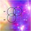 |
Fig. 3 Outline of the oversampled 6 × 6 regular map with 10′′ spacings of the O2 774 GHz observations. At this frequency, the beam of the 3.5 m Herschel telescope has a size of 28′′ (small blue circles). The beam centres for the H- and V-polarisations are separated by 4 |
In addition, the O2 line centroid and width also conform with values of other optically thin species, e.g.  (Liseau et al. 2010), N2H+ (1 − 0) (di Francesco et al. 2004), deuterated molecules (Bergman et al. 2011a) and the recently discovered H2O2 (HOOH, Bergman et al. 2011b). For the 2.8 km s-1 feature, we are unable to entirely exclude the possibility that it is due to an unidentified species. If so, the line transition frequency should be ν0 = (487250.548 ± 0.098) MHz (1σ).
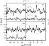 |
Fig. 4 The WBS spectra toward the positions O1 to O4 are shown for both the 774 GHz (upper) and 487 GHz (lower) lines in each frame. The average 774 GHz data are convolved to the 487 GHz beam of 44′′. Offsets relative to the origin O4 are shown along the upper and right-hand scales. |
3.2. 774 GHz
In Fig. 4 the convolved and averaged 774 GHz spectra are compared to the 487 GHz spectra, and the 6 × 6 map of the 774 GHz observations, convolved to the beam at 487 GHz, is displayed in Fig. 5. The line was not detected toward the east side of the cloud, i.e. toward O3 and O4, with 1σ-upper limits of 3 mK km s-1, but clearly detected toward the west side of the cloud, i.e. toward O1 and O2, at a signal-to-noise ratio of S/N = 4−6. The derived line parameters for the 774 GHz spectra, convolved to the 487 GHz beam, are reported in Table 3. We note that only the 3.6 km s-1 component is seen at the O1 position.
The O2 774 GHz line falls in the lower side band (LSB: 770.75−775.65 GHz). The entire observed spectral region is however totally dominated by the 13CO (7−6) transition at 771.2 GHz. This line exhibits significant variations on small angular scales, which is clearly evident in individual pointings of the 774 GHz beam of width 28′′ (FWHM). In the spectrum farthest to the northeast, the line reaches a peak Tmb of 25 K, whereas in the opposite corner in the southwest the intensity has decreased to less than 5 K.
In addition, in the upper side band (USB: 783.15−786.815 GHz), the strongest and clearly detected line is due to the C17O (7−6) transition at 786.3 GHz (Larsson et al., in prep.). In contrast to 13CO, the line of C17O reaches its maximum of almost 3 K at the O1 position.
4. Discussion
4.1. Observed quantities: temperature, line width, column density, and size of the O2 emission region
The O2 487 GHz and 774 GHz lines are clearly detected toward multiple positions. From the observation of more than one transition, some basic physical parameters of the source can be derived, where we assume that all transitions trace the same gas along the line of sight. In the case of the observed O2 emission, this should be straightforward, as detailed computations of statistical equilibrium and radiative transfer for a multi-level system demonstrate that this emission is optically thin and originates in conditions of local thermodynamic equilibrium (LTE).
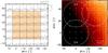 |
Fig. 5 Left: the regridded 6 × 6 map of the WBS 774 GHz spectra, weighted by the Gaussian profile of the 487 GHz beam of 44′′. The darker area shows roughly the region within the half power beam width (HPBW). The υLSR and TA scales are indicated in the upper right corner. Right: same as left panel but as an image of the spatial distribution of the integrated intensity, |

4.1.1. Temperature
At O1, the observed source extent of the 487 GHz and 774 GHz lines appears to be similar, hence the ratio of the beam fillings f487/f774 is probably not far from unity. In addition, the main beam efficiencies at these frequencies are also about equal (Table 1). Therefore, the observed ratio of integrated intensities I(487)/I(774)obs is directly comparable to the theoretical one, I(487)/I(774)theo, obtained from LTE calculations for optically thin O2 radiation, which depends only on the gas temperature (Fig. 7).
Observed O2 line intensity ratios.
From Table 4, we see that the measured intensity ratio of the 487 GHz to 774 GHz lines toward O1 implies a temperature of nearly 80 K, with the large error allowing a large range, from about 50 K to very much higher than 100 K (see also Fig. 7). If the beam filling at 774 GHz were smaller than that at 487 GHz, the actual temperatures would be even higher. Our value can be compared to earlier estimates, obtained at comparable spatial resolution, of both the dust and the gas temperature toward O1. From FIR continuum measurements with a 40′′ beam, Harvey et al. (1979) obtained the dust temperature Td = 41 K. Zeng et al. (1984) derived from NH3 observations, also with a 40′′ beam, the temperature of the gas, Tg ~ 45 K.
For the dense spot O4 (P 3, SM 1), the 3σ upper limit to the 774 GHz line yields a temperature that is strictly lower than 31 K, which would agree with the value of Tg = 22 ± 3 K obtained by Bergman et al. (2011b). For the dense core ρ Oph A, the average for ⟨ O1, O3, O4 ⟩ results in a value of about from 20 K to 25 K, which is entirely consistent with earlier determinations, based on a variety of techniques. Temperaturesbetween 9 K and 49 K have been derived, but with most values clustering around 20−30 K (e.g., Harvey et al. 1979; Loren et al. 1980; Ward-Thompson et al. 1989; Motte et al. 1998; Stamatellos et al. 2007; Bergman et al. 2011a; Ade et al. 2011).
As is also evident from Fig. 5, a temperature gradient or two distinctly different temperature regimes, i.e. higher than about 50 K and strictly lower than 30 K, exist within the boundaries of our limited map of roughly one square arcminute (see also Figs. 1 and 3).
4.1.2. Line width
Comparing the observed line widths, FWHM, of Table 3 with the resolutions offered by the HRS and WBS, we see that the HRS data for the 487 GHz line are all well-resolved (δυ = 0.15 km s-1), whereas the 774 GHz line toward O1 and O2 is just barely resolved with the WBS (δυ = 0.43 km s-1). However, the average 774 GHz spectrum ⟨ O1, O2 ⟩ is well-resolved with the HRS and the line has a comparable width to that observed with the WBS. It is remarkable that the lines in the cold regions O3 and O4 are observed to be broader than those in the warmer O1 and O2.
The non-thermal contribution to the observed width, Δυ = FWHM, of an unblended line is 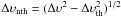 , where all radial velocities are expressed in terms of their FWHM. For T in the range 18 K to 30 K, Δυth = 0.27 to 0.35 km s-1, yielding Δυnth = 0.72 to 0.80 km s-1 for the cold region including O3 and O4 (Table 4). Hence, we find that there the line broadening is totally dominated by the non-thermal random motions, which are more than twice as high as the thermal ones. On the other hand, in the warm region O1 and O2, the thermal motions dominate over the non-thermal ones (0.57 km s-1 versus ≤ 0.44 km s-1 for T = 78 K) or are comparable at the lower limit temperature of 47 K. This could suggest that, if the non-thermal motions are identified with turbulence at O1 and O2, much of this turbulence has been dissipated and converted into heat.
The O2 source is seen in projection close to the outflow from VLA 1623 and judging from its position (Figs. 1 and 3), it is possible that the gas at O2 is enriched by shock-processed material. At the border of the outflow, a broader line might be expected due to enhanced turbulent motions. The 774 GHz line width appears (marginally) broader than that toward O1 (Table 3), but the uncertainties are large and the significance is low.
4.1.3. Source size
Having determined the temperature, we can use the theoretical line ratio for another transition and equate it to the ratio of the respective beam fillings, e.g. R ≡ (I119/I487)theo(T)/(I119/I487)obs = f487/f119. The relevant 119 GHz data were adopted from Larsson et al. (2007); they are compiled in Table 3 and all lines are displayed on the Tmb scale in Fig. 6. For a Gaussian beam at 119 GHz, the beam filling factor is given by 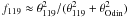 , where θ119 is the size of the source and θOdin that of the beam at 119 GHz. Re-arranging, this reads
  , where θOdin = 10′.
The 487 GHz source seems to be extended on the scale of at least the beam width, i.e. f487 ≥ 0.5, and for the average values of ⟨ O1, O3, O4 ⟩ in Table 4, we find a size of the Odin source of ≳ 4 to 5 arcmin, for gas at from 18 to 25 K, i.e. for (I119/I487)theo(T) = 11 to 8, respectively. The solution for much warmer gas (127 K for “ − 1σ” in Table 4) ought to be excluded, as the calculated source size would exceed 9′, whereas the 774 GHz line that traces high temperature has been detected only over a limited region ( ≲ 1′). On the basis of CS (2 − 1) mapping observations, Liseau et al. (1995) determined the deconvolved angular size of the densest regions of the ρ Oph A core as FWHM ~ 4′ (nH ≳ 105 cm-3), which is consistent with the HIFI and Odin observations of O2 in ρ Oph A taken together. It appears that the entire ρ Oph A core is faintly glowing in the 119 GHz line.
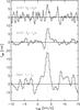 |
Fig. 6 Average data for the HIFI O2 observations (774 and 487 GHz) and the Odin 119 GHz spectrum toward ρ Oph A. For proper comparison, these spectra are given on the Tmb scale and for reference, a vertical dotted line is shown at υLSR = +3.5 km s-1. |
4.1.4. Column density
For the warm region O1, an O2 column density of 5 × 1015 cm-2 is derived, whereas for the cold O4, N(O2) > 6 × 1015 cm-2 (Table 4). These estimations are based on the assumption of optically thin emission in LTE at the kinetic gas temperature Tkin, i.e. for unit beam filling the O2 column is given by  when the integral is expressed in K cm s-1 and where
  in K-1 cm-3 s (cgs units throughout). Here, the transition temperature is Ttr ≡ hν/k, the quasi-Planck function is Fν(T) ≡ Ttr/(eTtr/T − 1), the partition function is Q(T), the upper level energy is Tup = Eup/k and the other symbols have their usual meaning. The background temperature is that of the cosmic microwave background, i.e. Tbg = TCMB1. The frequencies were adopted from Drouin et al. (2010) and the Einstein A-values from Maréchal et al. (1997) (see also Black & Smith 1984).
On the other hand, if ⟨ O1, O3, O4 ⟩ were taken as representative of ρ Oph A as a whole, column densities lower than 5 × 1015 cm-2 would be derived. Although there is a considerable range in gas kinetic temperature, the O2 column densities do not seem to vary that much. However, with the observed inhomogeneity of the emission in mind, the significance of such an average could be questioned.
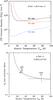 |
Fig. 7 Upper: LTE computations of the O2 column density N(O2) as a function of the temperature T for an extended homogeneous source, to yield a line intensity of 1.0 K km s-1. For optically thin emission, intensity and column density are linearly related. 119 GHz: blue dots; 487 Ghz: black solid line; 774 GHz: red short dashes. Lower: the ratio of the 487 GHz integrated line intensity to that at 774 GHz is shown by the curve for a range of temperatures. For O1 (=O1 |
4.2. O2 abundance
Once the O2 column density is known, the line-of-sight average O2 fractional abundance, with respect to H2 or H-nuclei, can be measured if the column density of H2 molecules is available. The hydrogen column density along the appropriate lateral and depth scales is not well-known from observations. However, we can get an approximate idea from the C18O observations by Liseau et al. (2010), where it was suggested, based on the line profiles, that the J = 3 − 2 line was a reasonably good proxy for the O2 119 GHz line observed with Odin (Larsson et al. 2007). If the O2 molecules were indeed cospatial with those of CO and its isotopic variants, their optically thin lines could be used to infer the H2 column densities relevant also to O2. We derive “local” C18O column densities by taking C18O intensity and O2 temperature variations into account. The gas and dust peaks coincide spatially (see also Table 2), i.e. there is no indication of significant CO freeze out (at levels higher than a factor of 2 to 3, see Fig. 10 of Bergman et al. 2011a). The C18O column density varies by less than 20% for 20 K ≤ Tkin ≤ 50 K. Assuming that C18O/H2 = 1.5 × 10⁻⁷ (likely within about 30%, e.g. Wannier et al. 1976; Goldsmith et al. 2000), H2 columns are found to be 1 × 1023 cm-2.
Hence, for the O2 column densities in Table 4, we find that X(O2) = 5 × 10⁻⁸ relative to H2 in the warm gas toward the west, at O1 (and likely also toward O2), and higher than that toward the east, at the colder O4. The C18O lines are slightly optically thick, implying that these H2 column densities are lower limits and need to be adjusted upwards by a factor of the order of τ/(1 − e − τ) ≳ 2, for τ ~ 2. Hence, these O2 abundances are upper limits, i.e. the fractional abundance of O2 in the gas phase is less than indicated above.
A way to obtain a more detailed picture of the source is to use detailed theoretical models to predict the O2 abundance or column and to compare these models with the observations. This is the topic of the next subsection.
4.3. Chemical models
Specifically for O2 (and H2O), Hollenbach et al. (2009) constructed theoretical models of photon-dominated regions (PDRs, Hollenbach & Tielens 1997), invoking also grain surface chemistry, including freeze-out and desorption of the species. These new models are models of the whole cloud, to arbitrary values of the extinction, and show that most of the gas phase O2, OH, and H2O is found at values of AV ~ 3 − 10 mag, where the details depend, as in a conventional PDR, on the ratio G0/nH. In many aspects, these models are similar to the traditional dense PDR models that include chemistry and gas heating and that explain the abundances and column densities of other molecules (including radicals and ions) at intermediate depths into the clouds (e.g., Fuente et al. 1993; Sternberg & Dalgarno 1995; Jansen et al. 1995; Simon et al. 1997; Pety et al. 2005). The current models are extended even deeper into the cloud where external UV photons no longer play a role in the chemistry, only cosmic-ray induced photons.
In the direction of ρ Oph A, a number of spectroscopic indicators suggest the presence of a PDR2. Liseau et al. (1999) inferred that the PDR is situated on the rear side of ρ Oph A, as seen from the Sun, and excited by the two stellar sources HD 147889 and S 1 (see Fig. 1 and Table 2) by their combined UV fields, corresponding to G0 ~ 102. For the densest parts of the [C II] emitting ρ Oph A-PDR, these authors empirically derived nH = 5 × 104 cm-3 and over more extended regions, from 1 to 3 × 104 cm-3.
The model of Hollenbach et al. (2009) predicts columns of O2 between about 1015 and a few times 1016 cm-2 depending on the grain temperature in the O2-emitting region, with higher columns in regions with warmer dust. Warmer (Td > 20 K) dust produces more O2 column because O atoms evaporate from grains before they can react with atomic hydrogen sticking to the grains. This increases the elemental gas phase O available to make O2, whose abundance in the ρ Oph model can locally reach above 10-5 for Td = 25 K. The results are quite insensitive to the gas temperature in the O2-emitting region for the range 10 K < Tg < 100 K.
However, the Hollenbach et al. (2009) models predict gas temperatures of only ~ 20 K, as would all thermochemical models with only cosmic ray heating and heating by the penetrating FUV. Gas temperatures as high as 80 K, as derived here, suggest that there are other heating mechanisms, such as slow shocks or turbulent dissipation (e.g., Goldsmith et al. 2010). Our observations show a slight increase in O2 column in cooler gas. If the dust is also cooler in the cooler gas region, as would be expected for the derived densities above 104 and, centrally, higher than 107 cm-3, this contradicts the predictions of this particular model.
On the other hand, geometry also plays a role in determining the column of O2 observed along the line of sight. The Hollenbach et al. (2009) models assume an illuminated slab face-on. However, clumpiness and more edge-on geometry could increase the observed column in some beams, and could explain the slightly higher column of O2 in the region with somewhat cooler gas. We conclude that these models are modestly consistent with the observations, but likely require some additional gas heating in the O2-emitting region. We defer detailed thermochemical modelling of these ρ Oph observations to a future paper.
4.4. Source(s) of O2 or the dearth of O2
The discussed models could be expected to apply quite generally to all externally illuminated molecular clouds developing PDR-like parts. It is therefore surprising that O2 has been detected only toward the dense cloud core ρ Oph A (Larsson et al. 2007, and this work) and a spot in OMC-1 (Goldsmith et al. 2011), despite numerous searches toward other regions. For instance, surveying twenty sources, Goldsmith et al. (2000) obtained limiting O2 abundances N(O2)/N(H2) of a few times 10-7, whereas Pagani et al. (2003) derived upper limits to the O2 column density of 1015 to a few times 1016 cm-2 for nearly a dozen objects. These surveys included dark clouds, regions of low-mass star formation in the solar neighbourhood and of high-mass star formation at different galactocentric distances, i.e. these surveys sampled a wide range of cloud properties and energetics, from quiescent cold clouds to turbulent shock-heated gas caused by mass infall and molecular outflows. Nevertheless, most of these regions escaped detection, although their limiting O2 column densities fall within the range predicted by the theoretical models.
One possibility could be that this apparent mismatch is due to observational bias, such as source distance and beam dilution. For instance, the limit on the O2 column in Ori A determined by Pagani et al. (2003) is entirely consistent with the HIFI beam-averaged detection obtained by Goldsmith et al. (2011), if proper correction for dilution in the Odin-beam is applied. We recall that the detected spot is not toward the Orion-PDR (Melnick et al. 2012), as one might have expected, but close to the outflow in the vicinity of IRc 2.
However, the difference in distance aside, ρ Oph A and Ori A represent very different environments in terms of the parameter G0/nH, viz. cold-core deuteration versus hot-core grain chemistry (Bergman et al. 2011a; Bisschop et al. 2007; Ceccarelli et al. 2007; Ratajczak et al. 2011). Star-forming regions such as IRAS 16293 in Ophiuchus, NGC 1333 in Perseus, or the Serpens core near S 68 are more akin to the conditions in ρ Oph A, yet no O2 detections have been reported. These complexes are at one to two times the distance to ρ Oph A, hence beam dilution issues should be unimportant. It is conceivable that the viewing geometry of ρ Oph A could be particularly favourable for the observability of O2, although this advantage may not be shared by other regions.
However, a clear difference is suggested by hydrogen peroxide (H2O2) only so far having been detected in ρ Oph A (Bergman et al. 2011b). H2O2 is thought to be a clear indicator of grain surface chemistry and relatively abundant at about 30 K (e.g., Cazaux et al. 2010).
In the specific model for ρ Oph conditions, Du et al. (2012) find that H2O2 is reasonably abundant only for some 105 yr (their Fig. 1). A similar, only slightly broader, profile is displayed by the abundance of O2, rendering this molecule essentially undetectable after about 2 × 10⁵ yr. Compared to other molecular species, which have attained chemical equilibrium and/or are abound on much longer timescales ( > 106 yr), the abundances of both H2O2 and O2 appear transient. Therefore, one may expect that the simultaneously detectable abundance of O2 and H2O2 could be used to infer the evolutionary chemical state of the cloud. If that is the case, this may also explain the paucity of known O2 line emitters.
5. Conclusions
We now summarise the main results of our present study:
-
We have successfully detected the 33−12 transition of O2 at 487 GHz with HIFI onboard Herschel toward three positions in the ρ Oph A core. In addition, we have also obtained a 6 × 6 oversampled map with 10′′ spacings in the 54 − 34 transition at 774 GHz.
-
The telescope pointings targeted two cold, high density cores, i.e. O4 [C18O P3 = SM 1] and O3 [C18O P2, near SM 1N], and two positions 30′′ west of these, labelled O2 and O1, respectively. All three observed positions (O1, O3 and O4) were detected in the 487 GHz line, with significant variations in the line intensity on scales as small as 30′′. At 774 GHz, emission was detected from only the western part of the map, including O1 and O2.
-
Combining the 487 GHz and 774 GHz data leads to the column density of N(O2) > 6 × 1015 cm-2, at the 3σ level and at T < 30 K, in the high density region O3 and O4, whereas in the warmer region of O1 and O2, N(O2) = 5.5 × 1015 cm-2 (T > 50 K). There, our standard analysis yields an abundance of N(O2)/N(H2) ~ 5 × 10⁻⁸ in the warm gas and somewhat higher in the cold region.
-
This result agrees with that for X(O2) based on the observation of the 119 GHz line with Odin (Larsson et al. 2007), assuming that the O2 source size has an angular extent of about 5′.
-
The question of why O2 is such an elusive molecule in the ISM is still unanswered. In the special case of ρ Oph A, there is some evidence that detectable amounts of gas phase O2 might be a relatively transient phenomenon, which could explain why interstellar O2 is generally not detected.
In our numerical radiative transfer calculations (Sect. 4.1), the dust continuum is also included. These calculations use the collision data of Lique (2010).
Atomic recombination lines of carbon, 12C, and sulfur, 32S, (Cesarsky et al. 1976; Pankonin & Walmsley 1978), fine structure lines: [C I] 492.2 GHz (Kamegai et al. 2003), [C I] 809.3 GHz (Kamegai et al. 2003; Kulesa et al. 2005), [C II] 157 μm (Yui et al. 1993; Liseau et al. 1999), [O I] 63 μm (Ceccarelli et al. 1997; Liseau et al. 1999), [O I] 145 μm (Liseau et al. 1999; Liseau & Justtanont 2009), and mid-infrared PAH emission (Liseau & Justtanont 2009).
Acknowledgments
We appreciate the thoughtful comments by the referee, Prof. Karl Menten, which have lead to an improvement of the manuscript. The Swedish authors are indebted to the Swedish National Space Board (SNSB) for its continued support. This work was also carried out in part at the Jet Propulsion Laboratory, California Institute of Technology, under contract with the National Aeronautics and Space Administration (NASA). We also wish to thank the HIFI-ICC for its excellent support. HIFI has been designed and built by a consortium of institutes and university departments from across Europe, Canada and the US under the leadership of SRON Netherlands Institute for Space Research, Groningen, The Netherlands with major contributions from Germany, France and the US. Consortium members are: Canada: CSA, U. Waterloo; France: CESR, LAB, LERMA, IRAM; Germany: KOSMA, MPIfR, MPS; Ireland, NUI Maynooth; Italy: ASI, IFSI-INAF, Arcetri-INAF; Netherlands: SRON, TUD; Poland: CAMK, CBK; Spain: Observatorio Astronomico Nacional (IGN), Centro de Astrobiologia (CSIC-INTA); Sweden: Chalmers University of Technology MC2, RSS & GARD, Onsala Space Observatory, Swedish National Space Board, Stockholm University Stockholm Observatory; Switzerland: ETH Zürich, FHNW; USA: Caltech, JPL, NHSC.
References
- Ade, P. A. R., Aghanim, N., Arnaud, M., et al. 2011, A&A, 536, A20 [NASA ADS] [CrossRef] [EDP Sciences] [Google Scholar]
- André, P., Martin-Pintado, J., Despois, D., & Montmerle, T. 1990, A&A, 236, 180 [NASA ADS] [Google Scholar]
- Bergman, P., Parise, B., Liseau, R., & Larsson, B. 2011a, A&A, 527, A39 [NASA ADS] [CrossRef] [EDP Sciences] [Google Scholar]
- Bergman, P., Parise, B., Liseau, R., et al. 2011b, A&A, 531, L8 [NASA ADS] [CrossRef] [EDP Sciences] [Google Scholar]
- Bisschop, S. E., Jørgensen, J. K., van Dishoeck, E. F., & de Wachter, E. B. M. 2007, A&A, 465, 913 [NASA ADS] [CrossRef] [EDP Sciences] [Google Scholar]
- Black, J. H., & Smith, P. L. 1984, ApJ, 277, 562 [NASA ADS] [CrossRef] [Google Scholar]
- Caratti o Garatti, A., Giannini, T., Nisini, B., & Lorenzetti, D. 2006, A&A, 449, 1077 [NASA ADS] [CrossRef] [EDP Sciences] [Google Scholar]
- Cazaux, S., Cobut, V., Marseille, M., Spaans, M., & Caselli, P. 2010, A&A, 522, A74 [NASA ADS] [CrossRef] [EDP Sciences] [Google Scholar]
- Ceccarelli, C., Haas, M. R., Hollenbach, D. J., & Rudolph, A. L. 1997, ApJ, 476, 771 [NASA ADS] [CrossRef] [Google Scholar]
- Ceccarelli, C., Caselli, P., Herbst, E., Tielens, A. G. G. M., & Caux, E. 2007, Protostars and Planets V, ed. B. Reipurth, D. Jewitt, & K. Keil (Tucson: University of Arizona Press), 47 [Google Scholar]
- Cesarsky, D. A., Encrenaz, P. J., Falgarone, E. G., et al. 1976, A&A, 48, 167 [NASA ADS] [Google Scholar]
- De Graauw, Th., Helmich, F. P., Phillips, T. G., et al. 2010, A&A, 518, L6 [NASA ADS] [CrossRef] [EDP Sciences] [Google Scholar]
- Dent, W. R. F., Matthews, H. E., & Walther, D. M. 1995, MNRAS, 277, 193 [NASA ADS] [Google Scholar]
- Di Francesco, J., André, P., & Myers, P. C. 2004, ApJ, 617, 425 [NASA ADS] [CrossRef] [Google Scholar]
- Du, F., Parise, B., & Bergman, P. 2012, A&A, 538, A91 [NASA ADS] [CrossRef] [EDP Sciences] [Google Scholar]
- Drouin, B. J., Yu, S., Miller, C. E., et al. 2010, JQSRT, 111, 1167 [Google Scholar]
- Elias, J. H. 1978, ApJ, 224, 453 [NASA ADS] [CrossRef] [Google Scholar]
- Frisk, U., Hagström, M., Ala-Laurinaho, J., et al. 2003, A&A, 402, L27 [NASA ADS] [CrossRef] [EDP Sciences] [Google Scholar]
- Fuente, A., Martin-Pintado, J., Cernicharo, J., & Bachiller, R. 1993, A&A, 276, 473 [NASA ADS] [Google Scholar]
- Goldsmith, P. F., & Langer, W. D. 1978, ApJ, 222, 881 [NASA ADS] [CrossRef] [Google Scholar]
- Goldsmith, P. F., Melnick, G. J., Bergin, E. A., et al. 2000, ApJ, 539, L123 [NASA ADS] [CrossRef] [Google Scholar]
- Goldsmith, P. F., Li, D., Bergin, E. A., et al. 2002, ApJ, 576, 814 [NASA ADS] [CrossRef] [Google Scholar]
- Goldsmith, P. F., Velusamy, T., Li, D., & Langer, W. D. 2010, ApJ, 715, 1370 [NASA ADS] [CrossRef] [Google Scholar]
- Goldsmith, P. F., Liseau, R., Bell, T. A., et al. 2011, ApJ, 737, 96 [Google Scholar]
- Grasdalen, G. L., Strom, K. M., & Strom, S. E. 1973, ApJ, 184, L53 [NASA ADS] [CrossRef] [Google Scholar]
- Harvey, P. M., Campbell, M. F., & Hoffmann, W. F. 1979, ApJ, 228, 445 [NASA ADS] [CrossRef] [Google Scholar]
- Hincelin, U., Wakelam, V., Hersant, F., et al. 2011, A&A, 530, A61 [NASA ADS] [CrossRef] [EDP Sciences] [Google Scholar]
- Hjalmarson, Å., Frisk, U., Olberg, M., et al. 2003, A&A, 402, L39 [NASA ADS] [CrossRef] [EDP Sciences] [Google Scholar]
- Hollenbach, D. J., & Tielens, A. G. G. M. 1997, ARA&A, 35, 179 [NASA ADS] [CrossRef] [Google Scholar]
- Hollenbach, D., Kaufman, M. J., Bergin, E. A., & Melnick, G. J. 2009, ApJ, 690, 1497 [CrossRef] [Google Scholar]
- Jansen, D. J., van Dishoeck, E. F., Black, J. H., Spaans, M., & Sosin, C. 1995, A&A, 302, 223 [NASA ADS] [Google Scholar]
- Johnstone, D., Wilson, C. D., Moriarty-Schieven, G., et al. 2000, ApJ, 545, 327 [NASA ADS] [CrossRef] [Google Scholar]
- Kamegai, K., Ikeda, M., Maezawa, H., et al. 2003, ApJ, 589, 378 [NASA ADS] [CrossRef] [Google Scholar]
- Kulesa, C. A., Hungerford, A. L., Walker, C. K., et al. 2005, ApJ, 625, 194 [NASA ADS] [CrossRef] [Google Scholar]
- Larsson, B., Liseau, R., Pagani, L., et al. 2007, A&A, 466, 999 [Google Scholar]
- Liseau, R., & Justtanont, K. 2009, A&A, 499, 799 [NASA ADS] [CrossRef] [EDP Sciences] [Google Scholar]
- Liseau, R., Lorenzetti, D., Molinari, S., et al. 1995, A&A, 300, 493 [NASA ADS] [Google Scholar]
- Liseau, R., White, G. J., Larsson, B., et al. 1999, A&A, 344, 342 [NASA ADS] [Google Scholar]
- Liseau, R., Larsson, B., Bergman, P., et al. 2010, A&A, 510, A98 [NASA ADS] [CrossRef] [EDP Sciences] [Google Scholar]
- Lique, F. 2010, J. Chem. Phys., 132, 04431 [Google Scholar]
- Loinard, L., Torres, R. M., Mioduszewski, A. J., & Rodríguez, L. F. 2008, ApJ, 675, L29 [NASA ADS] [CrossRef] [Google Scholar]
- Lombardi, M., Lada, C. J., & Alves, J. 2008, A&A, 480, 785 [NASA ADS] [CrossRef] [EDP Sciences] [Google Scholar]
- Loren, R. B., Wootten, A., & Wilking, B. A. 1990, ApJ, 365, 269 [NASA ADS] [CrossRef] [Google Scholar]
- Mamajek, E. E. 2008, Astron. Nachr., 329, 10 [Google Scholar]
- Maréchal, P., Viala, Y. P., & Benayoun, J. J. 1997, A&A, 324, 221 [NASA ADS] [Google Scholar]
- Melnick, G. J., Stauffer, J. R., Ashby, M. L. N., et al. 2000, ApJ, 539, L77 [NASA ADS] [CrossRef] [Google Scholar]
- Melnick, G. J., Tolls, V., Goldsmith, P. F., et al. 2012, ApJ, in press [Google Scholar]
- Motte, F., André, P., & Neri, R. 1998, A&A, 336, 150 [Google Scholar]
- Nord, H. L., von Schéele, F., Frisk, U., et al. 2003, A&A, 402, L21 [NASA ADS] [CrossRef] [EDP Sciences] [Google Scholar]
- Pagani, L., Olofsson, A. O. H., Bergman, P., et al. 2003, A&A, 402, L77 [NASA ADS] [CrossRef] [EDP Sciences] [Google Scholar]
- Pankonin, V., & Walmsley, C. M. 1978, A&A, 64, 333 [NASA ADS] [Google Scholar]
- Pety, J., Teyssier, D., Fossé, D., et al. 2005, A&A, 435, 885 [NASA ADS] [CrossRef] [EDP Sciences] [Google Scholar]
- Pilbratt, G. L., Riedinger, J. R., Passvogel, T., et al. 2010, A&A, 518, L1 [CrossRef] [EDP Sciences] [Google Scholar]
- Ratajczak, A., Taquet, V., Kahane, C., et al. 2011, A&A, 528, L13 [NASA ADS] [CrossRef] [EDP Sciences] [Google Scholar]
- Roelfsema, P. R., Helmich, F. P., Teyssier, D., et al. 2012, A&A, 537, A17 [NASA ADS] [CrossRef] [EDP Sciences] [Google Scholar]
- Simon, R., Stutzki, J., Sternberg, A., & Winnewisser, G. 1997, A&A, 327, L9 [NASA ADS] [Google Scholar]
- Snow, T. P., Destree, J., & Welty, D. E. 2008, ApJ, 679, 512 [NASA ADS] [CrossRef] [Google Scholar]
- Stamatellos, D., Whitworth, A. P., & Ward-Thompson, D. 2007, MNRAS, 379, 1390 [NASA ADS] [CrossRef] [Google Scholar]
- Sternberg, A., & Dalgarno, A. 1995, ApJ, 99, 565 [Google Scholar]
- Wannier, P. G., Penzias, A. A., Linke, R. A., & Wilson, R. W. 1976, ApJ, 204, 26 [NASA ADS] [CrossRef] [Google Scholar]
- Ward-Thompson, D., Robson, E. I., Whittet, D. C. B., et al. 1989, MNRAS, 241, 119 [NASA ADS] [Google Scholar]
- Yui, Y. Y., Nakagawa, T., Doi, Y., et al. 1993, ApJ, 419, L37 [NASA ADS] [CrossRef] [Google Scholar]
- Zeng, Q., Batrla, W., & Wilson, T. L. 1984, A&A, 141, 127 [NASA ADS] [Google Scholar]
All Tables
Source designations and coordinates for ρ Oph A, with positions observed in O2 in bold face.
All Figures
|
Fig. 1 Herschel beams of O2 487 GHz (44′′) superposed onto a grey scale C18O (3 − 2) map of ρ Oph A (Liseau et al. 2010). The + and × symbols designate the positions of the H- and V-polarization beam centres of HIFI, respectively, with a separation of 6 |
| In the text | |
|
Fig. 2 Average double side band (DSB) spectra of H- and V-polarizations for the three positions O1, O3, and O4 in the ρ Oph A cloud core, shown for the range 484.65 GHz to 489.85 GHz. The spectral lines are found exclusively in the lower side band (LSB) and the LSR velocity, υLSR, along the abcissa is in km s-1 and the antenna temperature TA along the ordinate in mK. a) 5 GHz wide band of the WBS around the 487 O2 line ( − 1600, + 1600 km s-1). b) The WBS spectrum at expanded scale, showing the O2 line at 487 GHz, which is detected in all three positions. Inspection of the individual on-off pairs suggests that the apparent absorption features next to the lines are not real but simply due to the noise. c) Similar to b) but for the corresponding HRS data. |
| In the text | |
|
Fig. 3 Outline of the oversampled 6 × 6 regular map with 10′′ spacings of the O2 774 GHz observations. At this frequency, the beam of the 3.5 m Herschel telescope has a size of 28′′ (small blue circles). The beam centres for the H- and V-polarisations are separated by 4 |
| In the text | |
|
Fig. 4 The WBS spectra toward the positions O1 to O4 are shown for both the 774 GHz (upper) and 487 GHz (lower) lines in each frame. The average 774 GHz data are convolved to the 487 GHz beam of 44′′. Offsets relative to the origin O4 are shown along the upper and right-hand scales. |
| In the text | |
|
Fig. 5 Left: the regridded 6 × 6 map of the WBS 774 GHz spectra, weighted by the Gaussian profile of the 487 GHz beam of 44′′. The darker area shows roughly the region within the half power beam width (HPBW). The υLSR and TA scales are indicated in the upper right corner. Right: same as left panel but as an image of the spatial distribution of the integrated intensity, |
| In the text | |
|
Fig. 6 Average data for the HIFI O2 observations (774 and 487 GHz) and the Odin 119 GHz spectrum toward ρ Oph A. For proper comparison, these spectra are given on the Tmb scale and for reference, a vertical dotted line is shown at υLSR = +3.5 km s-1. |
| In the text | |
|
Fig. 7 Upper: LTE computations of the O2 column density N(O2) as a function of the temperature T for an extended homogeneous source, to yield a line intensity of 1.0 K km s-1. For optically thin emission, intensity and column density are linearly related. 119 GHz: blue dots; 487 Ghz: black solid line; 774 GHz: red short dashes. Lower: the ratio of the 487 GHz integrated line intensity to that at 774 GHz is shown by the curve for a range of temperatures. For O1 (=O1 |
| In the text | |
Current usage metrics show cumulative count of Article Views (full-text article views including HTML views, PDF and ePub downloads, according to the available data) and Abstracts Views on Vision4Press platform.
Data correspond to usage on the plateform after 2015. The current usage metrics is available 48-96 hours after online publication and is updated daily on week days.
Initial download of the metrics may take a while.