| Issue |
A&A
Volume 541, May 2012
|
|
|---|---|---|
| Article Number | A15 | |
| Number of page(s) | 18 | |
| Section | Galactic structure, stellar clusters and populations | |
| DOI | https://doi.org/10.1051/0004-6361/201118381 | |
| Published online | 20 April 2012 | |
The double sub-giant branch of NGC 6656 (M 22): a chemical characterization⋆,⋆⋆
1
Max-Planck-Institut für Astrophysik
Karl-Schwarzschild-Str. 1
85741
Garching bei München
Germany
e-mail: This email address is being protected from spambots. You need JavaScript enabled to view it.
;
This email address is being protected from spambots. You need JavaScript enabled to view it.
; This email address is being protected from spambots. You need JavaScript enabled to view it.
2
Instituto de Astrofísica de Canarias, 38200 La Laguna, Tenerife, Canary Islands,
Spain
e-mail: This email address is being protected from spambots. You need JavaScript enabled to view it.
; This email address is being protected from spambots. You need JavaScript enabled to view it.
3
Department of Astrophysics, University of La Laguna,
38200 La Laguna, Tenerife,
Canary Islands,
Spain
4
Department of Astronomy and McDonald Observatory, The University
of Texas, Austin,
TX
78712,
USA
e-mail: This email address is being protected from spambots. You need JavaScript enabled to view it.
5
UCO/Lick Observatory, Department of Astronomy and Astrophysics,
University of California, Santa
Cruz, CA
95064,
USA
e-mail: This email address is being protected from spambots. You need JavaScript enabled to view it.
6
Department of Astronomy, University of Washington,
Seattle, WA
98195,
USA
e-mail: This email address is being protected from spambots. You need JavaScript enabled to view it.
7
INAF – Osservatorio Astronomico di Teramo, via M. Maggini,
64100
Teramo,
Italy
e-mail: This email address is being protected from spambots. You need JavaScript enabled to view it.
8
Research School of Astronomy & Astrophysics,
Australian National University, Mt Stromlo Observatory, via Cotter Rd, Weston, ACT
2611,
Australia
e-mail: This email address is being protected from spambots. You need JavaScript enabled to view it.
9
INAF – Osservatorio Astronomico di Padova, Vicolo
dell’Osservatorio 5, 35122
Padova,
Italy
e-mail: This email address is being protected from spambots. You need JavaScript enabled to view it.
10
European Southern Observatory, Karl-Schwarzschild-Str. 2, 85748
Garching bei München,
Germany
e-mail: This email address is being protected from spambots. You need JavaScript enabled to view it.
11
European Southern Observatory, Alonso de Cordova 3107, Santiago, Chile
e-mail: This email address is being protected from spambots. You need JavaScript enabled to view it.
12
Dipartimento di Astronomia, Università di Padova,
Vicolo dell’Osservatorio 3,
35122
Padova,
Italy
e-mail: This email address is being protected from spambots. You need JavaScript enabled to view it.
13
Carnegie Observatories, 813 Santa Barbara Street, Pasadena, CA
91101,
USA
e-mail: This email address is being protected from spambots. You need JavaScript enabled to view it.
14
Herzberg Institute of Astrophysics, National Research Council Canada, 5071 West Saanich Road,
Victoria, BC
V9E 2E7,
Canada
e-mail: This email address is being protected from spambots. You need JavaScript enabled to view it.
15
Pontificia Universidad Católica de Chile, Departmento de
Astronomía y Astrofisíca, Casilla
306, Santiago 22,
Chile
e-mail: This email address is being protected from spambots. You need JavaScript enabled to view it.
Received:
2
November
2011
Accepted:
11
February
2012
Abstract
We present an abundance analysis of 101 subgiant branch (SGB) stars in the globular cluster M 22. Using low-resolution FLAMES/GIRAFFE spectra we have determined abundances of the neutron-capture strontium and barium and the light element carbon. With these data we explore relationships between the observed SGB photometric split in this cluster and two stellar groups characterized by different contents of iron, slow neutron-capture process (s-process) elements, and the α element calcium, which we previously discovered in M 22’s red-giant stars. We show that the SGB stars correlate in chemical composition and the color–magnitude diagram position. The stars with higher metallicity and relative s-process abundances define a fainter SGB, while stars with lower metallicity and s-process content reside on a relatively brighter SGB. This result has implications for the relative ages of the two stellar groups of M 22. In particular, it is inconsistent with a broad spread in ages of the two SGBs. By accounting for the chemical content of the two stellar groups, isochrone fitting of the double SGB suggests that their agesare not different by more than ~300 Myr.
Key words: techniques: spectroscopic / stars: abundances / stars: Population II / globular clusters: individual: NGC 6656
Based on data collected at the European Southern Observatory with the FLAMES/GIRAFFE spectrograph under the program 085.D-0698A.
Tables 2 and 3 are available in electronic form at http://www.aanda.org
© ESO, 2012
1. Introduction
Thanks to the large amount of spectroscopic and photometric data assembled in the last couple of decades, the assumption that all globular clusters (GCs) contain a simple monometallic stellar population must be modified. Nearly all GC stars exhibit substantial star-to-star variations in light elements, mainly C, N, O, Na, Mg, and Al (e.g., Kraft 1994; Ramírez & Cohen 2002; Gratton et al. 2004). These anomalous abundances appear to be present in stars of all evolutionary states, including convectively unmixed subgiant branch (SGB) and main-sequence turnoff stars. This argues that many of the variations were in the birth material of the stars we see today. The light element abundances have various correlations and anticorrelations that point unmistakably to hot H-burning ON, NeNa, and MgAl proton-capture chains. These cannot be products of the present low-mass GC stars, so it is probable that a fraction of GC stars are made up of material processed through higher mass stars that are now compact objects in the GCs. Multiple stellar generations in GCs are therefore needed (e.g., Marino et al. 2008; Carretta et al. 2009).
In clusters that we may call normal GCs, stellar abundances of elements heavier than those affected by H-burning show both intra- and inter-cluster consistency, and their abundances resemble the halo field compositions at similar overall metallicities. For these GCs, a two-generation model is sufficient: a primordial generation similar to the field, and stars formed as second generation(s) enriched in material processed through hot H-burning. Powerful photometric tools to separate these stellar generations along the RGBs include the Johnson U band and specific Strömgren indices (Marino et al. 2008; Yong et al. 2008). The accepted cluster evolutionary scenario is that normal GCs have been polluted with hot H-burning products by first-generation asymptotic giant branch stars (AGB, Ventura et al. 2001; D’Antona & Caloi 2004), and/or fast rotating massive stars (Decressin et al. 2007). Massive binaries have also been proposed as an alternative source (de Mink et al. 2009; Vanbeveren et al. 2011). Stars formed as second-generation members were born from the material released by these proposed first-generation polluters.
Recent spectroscopic studies have revealed that some GCs have variations not only in light elements, but also in the bulk heavy-element content. These clusters, which we designate as anomalous GCs (AGCs), have significant metallicity dispersions (star-to-star variations in Fe-peak abundances). GCs that have displayed this anomalous behavior include NGC 6656 (M 22, Marino et al. 2009), NGC 2419 (Cohen et al. 2010), Terzan 5 (Ferraro et al. 2009), and NGC 1851 (discovered by Yong & Grundahl 2008; and confirmed by Carretta et al. 2010, 2011). All these objects share superficial similarities to the most massive GC ω Centauri, whose huge metallicity variations have been known since the 1970s (e.g. Dickens & Wooley 1967; Freeman & Rodgers 1975; and more recently Norris & Da Costa 1995; Suntzeff & Kraft 1996; Johnson & Pilachowski 2010; Marino et al. 2011b). Omega Cen shows a very broad metallicity distribution that could be consistent with five to six groups of stars with different metallicities, as both spectroscopic and photometric studies seem to suggest (Johnson & Pilachowski 2010; Marino et al. 2011b; Sollima et al. 2005; Bellini et al. 2010). The ω Cen metallicity spread is so wide that it may have a different origin from the other GCs. It could be the surviving nucleus of a dwarf galaxy tidally disrupted by the Milky Way, as suggested by Bekki & Norris (2006). Unlike the simple normal GCs, in these objects successive generation(s) may need to be invoked, with supernovae also playing a role in polluting intracluster medium.
In the AGCs NGC 1851 and M 22, different groups of stars with different slow-process (s-process) element abundances have been identified (Yong & Grundahl 2008, for NGC 1851; and Marino et al. 2009, 2011a, for M 22, hereafter M09 and M11a respectively). Multiple stellar groups in M 22 and NGC 1851 are also clearly manifest by a split in their SGB color–magnitude diagram domains, as revealed by Hubble Space Telescope (HST) images (Milone et al. 2008; M09; Piotto 2009). The split SGB in these two clusters appears to be related to chemical differences observed among their red-giant branch (RGB) stars.
The chemical complexities in M 22 RGB stars have been extensively studied by M09 and M11a. They show that this cluster hosts two metallicity groups, with mean abundances ⟨ [Fe/H] ⟩ = −1.82 (σ = 0.07) and −1.67 (σ = 0.05). These two metallicity groups are characterized principally by different relative contents of the n-capture elements that can be efficiently synthesized in the s-process; that is, ⟨ [Y, Zr, Ba, La, Nd/Fe] ⟩ = −0.01 (σ = 0.06) in the lower metallicity group and +0.35 (σ = 0.06) in the high metallicity group. On the other hand, Eu which is predominantly synthesized in the r-process, exhibits constant relative abundances, within the observational errors: ⟨ [Eu/Fe] ⟩ = + 0.49 (σ = 0.05) in the lower metallicity group and +0.42 (σ = 0.08) in the higher one. This clearly indicates that the higher n-capture element content in the higher metallicity M 22 RGB stars is due to addition of material produced via the s-process. The two stellar groups were named s-rich and s-poor by M09, and we follow that convention here.
For M 22, M09 also demonstrates that stellar models cannot entirely reproduce the size of the SGB photometric split by considering only its metallicity spread. They suggest that the origin of the split could be more complex and also involves a difference in age and/or variations in the total CNO abundance, as proposed by Cassisi et al. (2008) and Ventura et al. (2009) for NGC 1851. This scenario is supported by observational evidence of total C+N+O variations among RGB stars both in NGC 1851 (Yong et al. 2009) and M 22 (M11a).
Although photometric evidence of the population multiplicity of M 22 is most clearly evident in the SGB domain, previous detailed abundance studies only have been carried out for the brighter RGB and AGB stars. In this study we eliminate this sample mismatch by performing a chemical composition analysis of 101 SGB stars in M 22. The layout of this paper is as follows: Sect. 2 is an overview of the data set; Sect. 3 contains a description of model atmospheres and abundance derivations; Sect. 4 presents the abundance results, which are discussed in Sects. 5 and 6. The findings of this paper are summarized in Sect. 7.
2. Observations and data reduction
Basic information for M 22 can be found in Harris (1996)1. At a distance of ~3.2 kpc M 22 is one of the GCs that are closest to the Sun. It has a half-light radius of 3.36′ and a mass of  , as listed in Mandushev et al. (1991). In this section we consider in turn the photometric and spectroscopic data that we have employed in this study.
2.1. The photometric dataset
We first establish that the SGB of M 22 is photometrically split in a manner that mimics the division already established among the RGB (M11a). We then consider three distinct sets of photometry available in the literature, in order to investigate the distribution of spectroscopic targets in the color–magnitude diagram (CMD). Ground-based observations were used to analyze the CMD over a wide spatial field in the B and V bands and to estimate the atmospheric parameters of the spectroscopic targets. In addition, we used ground-based U images available for a smaller field, and images taken with the Advanced Camera for Surveys onboard the HST (ACS/HST; Clampin et al. 2002, and references therein) in the F606W and F814W bands to make our study of the double SGB extend from the ultraviolet to the infrared spectral regions.
The HST ACS/WFC images were obtained under program GO-10775 (PI Sarajedini). The data sets consist of (short exposure, deep exposures) = 3 s, 4 × 55 s in F606W, and 3 s, 4 × 65 s in F814W. We used the photometric catalogs provided by Anderson et al. (2008) reduced as described in Anderson & King (2006).
Ground-based photometric database.
The ground-based photometric database consists of a total of 533 individual CCD images taken with different telescopes (see Table 1). These images were taken as part of P. B. Stetson’s program to produce a large homogeneous GC database. The images were reduced and calibrated as described in detail by Stetson (2000, 2005). The final photometric catalog covers a total field of view of ~34′ × 33′ and contains 730 432 entries; of these, 604 979 objects had enough data to allow calibration in at least V and one other filter. We used the B and V magnitudes from this catalog.
In addition to this wide-field catalog, we used a separate photometric catalog derived from images collected by the SUperb-Seeing Imager (SUSI2) camera, previously mounted on the ESO-NTT telescope (Table 1). The SUSI2 camera was a mosaic of two 2k × 4k,  pixel CCDs, where each chip covered a field of view of
  . The photometric reduction and calibration of this dataset was presented in Momany et al. (2004). The U and V magnitudes are available in this catalog.
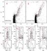 |
Fig. 1 Comparison of the U versus (U − V) CMD from NTT photometry (Momany et al. 2004) before (panel a)) and after (panel b)) the correction for differential (but not for the absolute) reddening. The horizontal branch stars lie at U ~ 17. The Δ(U − V) distributions of RGB stars with respect to the fiducial (red dash-dotted line on the CMDs) are shown in panels c) and d) for the uncorrected CMD, and in panels g) and h) for the corrected one. For SGB stars we show the distributions of the ΔU magnitude relative to the fiducial shown in the CMDs for the uncorrected (panels e) and f)) and the corrected (panels i) and l)) CMDs. |
Since we were interested only in target stars with high-accuracy photometry, we included in our analysis only relatively isolated stars with good values of PSF-fit quality indices and small errors in photometry and astrometry. A detailed description of the selection procedures is given in Milone et al. (2009).
M 22 has an average reddening E(B − V) = 0.34 (Harris 1996); such a high reddening value is rarely uniform over a cluster face. Corrections for differential reddening applied to the HST GC dataset is discussed in detail by Piotto et al. (2012) for M 22. To account for the color and magnitude differences that differential reddening produces in the ground-based CMDs, we used the procedure described by Milone et al. (2012). We first drew a main-sequence ridge (fiducial) line by putting a best-fit spline through the median colors found in successive short intervals of magnitude. We iterated this step with an outlier sigma clipping. Then for each program star, we estimated how much the observed stars in its spatial vicinity systematically lie to the red or the blue of the fiducial sequence. This systematic color and magnitude offset, measured along the reddening line, is indicative of the local differential reddening.
We corrected for differential reddening all of the HST and ground-based color–magnitude diagrams used in this paper. As an example, in Fig. 1, we compare the original (panel a) and the corrected U-(U − V) CMD (panel b) of M 22 for the SUSI2/NTT photometry from Momany et al. (2004). The choice of this combination of magnitude and color is due to its ability to separate photometric sequences at different evolutionary stages along the CMD. The blue and near-UV regimes of cool-star spectra contain many CH and CN molecular features. Stars with different amounts of these elements populate different RGB sequences in CMDs constructed by using the U-band (Marino et al. 2008).
Inspection of Fig. 1 shows that after the differential reddening correction has been applied, many features of the CMD became narrower and more clearly defined. To better demonstrate the quality of this correction we performed some tests represented in the lower panels of Fig. 1. We drew the fiducials for the brighter SGB and bluer RGB population by hand, and superimposed them on the CMDs. For each RGB star, we calculated the color difference Δ(U − V) from the fiducial at a given U magnitude, while for the SGB stars we calculated the difference in the U magnitude at a given color. These color and magnitude differences, as well as histogram plots, are represented in the lower panels of Fig. 1. The verticalized U versus Δ(U − V) diagram is plotted in panels c and g for RGB stars with 17.5 < U < 19.4 by using original and corrected photometry, respectively. The corresponding histogram color distributions are shown in panels d and h.
Panels e and i of Fig. 1 show the (U − V) versus ΔU diagram for SGB stars with 2.90 < (U − V) < 3.15 obtained from original and corrected magnitudes, respectively. The corresponding histogram color distributions are plotted in panels f and l. The better separation of the SGB and RGB sequences in the corrected diagram suggests that differential reddening has been substantially removed. Our differential reddening correction shows that the maximum values of ΔE(B − V) are approximately of 0.1 mag across the face of the cluster.
Examination of the reddening-corrected U versus (U − V) diagram (panel (b) of Fig. 1) clearly reveals that the bright SGB is connected to the blue RGB, while red RGB stars are the progeny of the faint SGB. We anticipate that this connection between the two SGBs and RGBs would be further confirmed by our M 22 SGB investigation, and we explore these relationships in Sect. 5.
2.2. The spectroscopic dataset
Our spectroscopic data consist of a large number of FLAMES/GIRAFFE spectra (Pasquini et al. 2002, 2003) observed under the program 085.D-0698A (PI: Marino). The low-resolution LR02 GIRAFFE setup was employed, which covers a spectral range of ~600 Å from 3964 Å to 4567 Å, and provides a resolving power R ≡ λ/Δλ ~ 6400. All our target stars were observed in the same FLAMES plate in four different exposures of 46 min plus one exposure of 26 min, for a total observing time of 210 min. The typical S/N of the fully reduced combined spectra is ~90−100 at the central wavelength of the spectral range. Data reduction involving bias subtraction, flat-field correction, wavelength calibration, and sky subtraction is done by using the dedicated pipeline BLDRS v0.5.32.
In total we gathered spectra for 109 candidate M 22 SGB stars. The M 22 SGB stars lie in a (B − V) color region ranging from ~0.8 to ~1, and extend in V magnitude from ~17.8 up to ~16.7. Cluster membership of the stars was established from the radial velocities obtained using the IRAF FXCOR task, which cross-correlates the object spectrum with a template. For the template we used a synthetic spectrum obtained through the spectral synthesis code SPECTRUM (Gray & Corbally 1994)3. This spectrum was computed with a model stellar atmosphere interpolated from the Kurucz (1992) grid4, adopting parameters (Teff, log g, ξt, [Fe/H]) = (6000 K, 3.5, 1 km s-1, −1.70). Observed radial velocities were corrected to the heliocentric system. The observed/template spectrum matches, after the heliocentric correction, yielded for the whole sample a mean radial velocity of −143 ± 1 km s-1 (σ = 9 km s-1). This value agrees reasonably with the values in the literature (e.g., −148.8 ± 0.8 km s-1, σ = 6.6 km s-1, Peterson & Cudworth 1994; −146.3 ± 0.2 km s-1, σ = 7.8 km s-1, Harris 1996). Then we rejected individual stars with values deviating by more than 3σ from this average velocity, deeming them to be probable field stars. After rejecting these field stars, our sample of bona fide cluster stars is composed of 101 SGBs.
Basic UBVI photometry for the M 22 spectroscopically analyzed stars is listed in Table 2, where we list the coordinates, the original U, B, V, and I magnitudes from the ground-based photometry, and the differential reddening correction ΔE(B − V) applied to each target.
3. Data analysis
3.1. Atmospheric parameters
Chemical abundances were derived from a local thermodynamic equilibrium (LTE) analysis by using the latest version of the spectral analysis code MOOG (Sneden 1973)5. Effective temperatures (Teff) were estimated by using the Casagrande et al. (2010) (B − V)-Teff calibrations (based on the “infrared flux method”) for main sequence and subgiant stars. Our colors were corrected for the mean M 22 reddening after accounting for differential reddening effects as described in Sect. 2.1. Indeed, as discussed in Casagrande et al. (2010), accurate reddening corrections are crucial for determining Teff via the infrared flux method: a shift of only + 0.01 mag in E(B − V) translates into a Teff change of about + 50 K. In the case of M 22, differential reddening effects are quite large, and, if left uncorrected, they would yield (B − V)-based Teff errors up to ~500 K. After applying the differential reddening corrections, we estimate that our internal color uncertainties are ≈0.01−0.015 mag, implying internal uncertainties of ~100 K in Teff. Of course, some stars in our sample, mainly those in the central crowded field of the cluster where the ground-based photometry is not good, have larger photometric errors. For these stars we expect to have larger errors in the colors that translate into larger internal errors in the derived temperatures.
Surface gravities (log g) were obtained from the apparent V magnitudes, the above Teff, assuming a mass M = 0.80 M⊙, bolometric corrections from Alonso et al. (1999), and an apparent distance modulus of (m − M)V = 13.60 (Harris 1996, 2010 updated). This value agrees with the one obtained by our best isochrone-fit value, (m − M)V = 13.64 (Piotto et al. 2012). Gravities derived in this manner are affected mainly by the adopted distance modulus and mass, whose variations systematically change the surface gravities. An internal variation of ~0.1 in the adopted stellar masses modifies log g values of ~0.05 dex, with lower gravities for lower masses. Such minor excursions in log g do not significantly affect the abundances derived in this paper (see the error analysis in Sect. 3.2). The derived values for Teff and log g are listed in Table 3. They span a range of ~900 K and ~0.70, respectively.
Microturbulent velocities cannot be independently determined from our spectra or photometry, so we adopted the Gratton et al. (1996) prescription:  (1)However, since all our SGB stars have similar gravities, this relation predicts very similar ξt values, with a mean ⟨ ξt ⟩ = 0.97 ± 0.01 km s-1 (σ = 0.04). Therefore we assumed a uniform microturbulence of 1.0 km s-1 for all our targets.
For the metallicity of our model atmospheres we used the results of M09 and M11a in a general way, derived from their analysis of high-resolution spectra of a large sample of RGB stars. Those papers demonstrate that M 22 hosts two groups of stars, one that is s-rich and one that is s-poor, with different metallicities by a mean [Fe/H] variation of ~0.15 dex. The different metallicities are accompanied by large difference in s-process elemental abundances, with the s-rich stars having higher metallicity with respect to the s-poor stars. Given the relatively low resolution of our spectra, it is very difficult to detect such small metallicity variations in our SGB program stars. A difference of 0.15 dex in metallicity does not lead to significant departures in the relevant model atmosphere quantities (such as opacity). Nevertheless, in our analysis we have accounted for this difference by using the following procedure. (i) First we adopted the mean metallicity of the cluster, [A/H] = −1.76 (M09 and M11a), as the metallicity for a given star. (ii) Then we derived the stars’s abundance of Sr, an element whose abundance in the Solar System is predominantly produced by the s-process. (iii) With an estimate of the s-process content of each star, we adopted the mean metallicity obtained in our previous work for the s-rich and s-poor stars in its final model atmospheres: [A/H] ≈ −1.67 for the s-rich stars, and [A/H] ≈ −1.82 for s-poor ones (see Table 7 in M11a).
In Fig. 2 we show two averaged spectra, covering three Fe i lines, obtained from a sample of s-rich and s-poor stars (see Sect. 4 for more details). On each observed line we have superimposed two synthetic spectra with appropriate atmospheric parameters, but one with [Fe/H] = −1.67 (the mean metallicity of s-rich stars) and the other with [Fe/H] = −1.82 (the mean metallicity of s-poor stars). The averaged s-poor star is consistent with having a lower metallicity than the s-rich one, and the level of the Fe difference is similar to the one that M09 and M11a found in RGB stars. However, the line strength differences are small, illustrating the difficulty of determining the small difference in metallicity among s-rich and s-poor SGB stars from our individual spectra.
The contributions to the continuum source function due to Thomson+Rayleigh scattering effects are small at our metallicity-temperature-gravity regime for our spectral lines. Indeed, we verified that the differences in Sr, Ba, and C abundances obtained with the scattering and non-scattering versions of our synthetic spectrum code MOOG are negligible. Therefore, we used the code version that does not take scattering into account.
To keep the present analysis consistent with our previous work on M 22, we used interpolated model atmospheres from the grid of Kurucz (1992), with fixed Teff, log g, ξt, and metallicity. These models were constructed by including convective overshooting. Our trial syntheses suggest that the use of these models produces an overestimation of ~0.10 dex in all abundances compared with those determined with model atmospheres from Castelli & Kurucz (2004), which do not assume convective overshooting. We emphasize that the metallicity assumptions had little influence on establishing the s-richness of individual stars. These were accomplished almost exclusively by the Sr abundances. More details on the segregation of stars on basis of s-element content are given in Sect. 4.1.
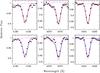 |
Fig. 2 Fe i lines for the combined s-poor (lower) and s-rich (upper) spectra of Fig. 7. Superimposed on the observed spectra are synthetic spectra corresponding to the [Fe/H] = −1.67 (red), [Fe/H] = −1.82 (blue), and with no Fe (magenta). |
 |
Fig. 3 Observed and synthetic spectra around the Sr lines at 4077 Å and 4215 Å and the G band for the s-rich star #2505. In each panel the points represent the observed spectrum, and the continuous lines are the synthesis computed with different strontium and carbon abundances. The magenta line is the spectrum computed with no contribution from Sr ii and C; the red line is the best-fitting synthesis (with the abundances given in Table 3); and the green and blue lines are the syntheses computed with Sr and C abundances altered by ± 0.3 dex from the best value. |
3.2. Chemical abundances
Using the model atmospheres and analysis code described in Sect. 3.1, we determined abundances for the neutron-capture (n-capture) elements Sr and Ba and for light element C. Limited by the relatively low resolution and the small wavelength range of our spectra, we derived Sr and Ba abundances only from the strong resonance transitions Sr ii 4077, 4215 Å, and Ba ii 4554 Å. Both the Sr lines suffer from many blends with other surrounding transitions, mostly Fe features and also other n-capture species (Dy and La) in the case of the Sr ii 4077. Spectral synthesis in the analysis of these lines (and particularly at our moderate resolution) is needed to take these blends into account. Although the Ba ii 4554 Å is isolated from contaminating transitions, we also computed synthesis for the Ba spectral line, to take its isotopic splitting into account. The linelists are based on Kurucz line compendium6, apart from the Ba transition for which we added hyperfine structure and isotopic data from Gallagher et al. (2010). For Sr our linelists neglect hyperfine/isotopic splitting, the wavelength shifts are very small, and Sr has one dominant isotope.
The resonance lines of Sr ii and Ba ii are formed relatively far out in the atmosphere, and, according to our NLTE calculations, are affected by departures from LTE (see e.g. Bergemann & Gehren 2008, for details on these calculations). Here, we note that Sr ii and Ba ii are the majority ions of their elements in the atmospheres of late-type stars (as also demonstrated by Short & Hauschildt 2006), and the major deviations from LTE are due to the non-equilibrium excitation effects in the line transitions. In particular, deviation of the line source functions from the Planck function leads to the NLTE profile strengthening, thus requiring somewhat lower abundances to fit observed spectral lines. For further details on the NLTE effects affecting our lines, we refer the reader to Bergemann et al. (in prep.). Here, we use these NLTE corrections to estimate how much our abundances could be affected by these effects. According to our NLTE calculations, we estimated NLTE corrections to range from −0.12 to + 0.04 dex for the Ba ii 4554 Å line, and only from −0.05 to 0.00 dex for the two Sr ii lines.
An additional difficulty in the analysis of Ba is that it has five major naturally occurring isotopes whose production fractions in the rapid-process (r-process) and s-process are significantly different (e.g., Kappeler et al. 1989). In particular, abundances derived from the Ba ii 4554 Å transition are very sensitive to the adopted r/s fraction (e.g. Mashonkina & Zhao 2006; Collet et al. 2009). This is an issue in the analysis of M 22, which hosts stars with different contribution from the s-process material, as demonstrated in M09 and M11a.
The M 22 s-poor stars have n-capture abundance distributions that are compatible with pure r-process material, as shown in Roederer et al. (2011). Since the s-rich stars should have a larger nucleosynthetic contribution from the s-processes (recalling that within observational errors, Eu is constant in the two M 22 s-groups), a two-step abundance analysis needed to be adopted. We first determined Ba abundances by adopting a scaled solar-system Ba abundance and isotopic fractions (Lodders 2003) for all the stars in our sample. Then the initial Sr syntheses were used to divide the total sample into s-poor and s-rich groups of stars (as discussed further in Sect. 4.1). Finally we recalculated the Ba abundances of the s-poor stars, assuming a pure r-process isotopic ratio (Arlandini et al. 1999). The recomputed Ba abundances in s-poor stars are lower by ~0.20 dex than the ones obtained in our first abundance estimates. Of course a similar systematic shift towards lower Ba abundances is also obtained for the s-rich stars if a pure r-process isotopic ratio is assumed. However, for the s-rich stars, we kept our original Ba abundance values, because the solar-system isotopic fractions for the s-rich stars appear to be a good approximation. This is justified since M11a showed that the M 22 s-rich RGB stars have a solar-system n-capture-element mix; i.e., [Y, Zr, Ba, La, Nd/Eu] ≈ 0.
Carbon was measured from spectral synthesis of the CH (A2Δ − X2Π) G-band heads near 4314 and 4323 Å. The molecular line data employed for CH were provided by B. Plez (priv. comm.; some basic details of the linelist are given in Hill et al. 2002). As an example, we show in Fig. 3 the spectral synthesis of the Sr lines and the G band for the s-rich star #2505 (Teff = 5923 K, log g = 3.97, [A/H] = −1.67). A list of the derived chemical abundances, together with the atmospheric parameters, is provided in Table 3.
An internal error analysis was accomplished by varying the temperature, gravity, metallicity, and microturbulence one by one, and re-determining the abundances for three stars spanning the entire range in Teff. The parameters were varied by ΔTeff = ± 100 K, Δlog g = ± 0.2, Δ[Fe/H] = ± 0.1, and Δξt = ± 0.2, typical uncertainties associated with our atmospheric parameters. The contribution of continuum placement errors was estimated by determining the change in abundances as the synthetic/observed continuum normalization was varied: generally this uncertainty added 0.10 dex to the abundances. The various errors were added in quadrature, resulting in typical uncertainties of ≈ 0.15 for the C abundances, ≈0.25 for the individual Sr line abundances, and ≈0.22 dex for Ba. The standard errors σ associated with the mean Sr abundances obtained from the two available spectral lines, are listed in Table 3. The mean of these σ values, which is 0.08 ± 0.01, is an estimate of the error associated with the mean Sr abundance of each star. Systematic effects could affect our atmospheric parameters, which would lead to systematic abundance differences that could be larger than those introduced by internal uncertainties. However, we are only interested here in relative star-to-star chemical variations among a set of M 22 SGB stars with a restricted parameter range. This renders systematic abundance uncertainties unimportant for our purposes. Investigation of such systematics is worth pursuing in the future, but is beyond the aims of our work here.
4. Results
Our results for C, Sr, and Ba abundances in all program stars are listed in Table 3. These three elements all show a wide spread that cannot be entirely accounted for by observational errors. The mean abundances for all the analyzed stars are ⟨ [C/H] ⟩ = −1.75 (⟨ [C/Fe] ⟩ = 0.00, σ = 0.22, for 100 stars); ⟨ [Sr/H]NLTE ⟩ = −1.66 (⟨ [Sr/Fe]NLTE ⟩ = 0.10, σ = 0.21, for 101 stars); and ⟨ [Ba/H]NLTE ⟩ = −1.63 (⟨ [Ba/Fe]NLTE ⟩ = 0.13, σ = 0.26, for 100 stars).
For strontium and barium the mean abundances are those corrected for NLTE. In the following we discuss the spreads of each single element.
4.1. Strontium
In Fig. 4 we plot the LTE and NLTE Sr abundances for our program stars, both in “absolute” log ϵ units and relative [Sr/Fe] ratios. The wide spreads in Sr that we observe here are consistent with our findings on RGB stars. The small NLTE corrections make no significant alterations to these spreads. No Sr abundances were reported in M09 and M11a. However, the Sr distribution for our SGB sample is clearly bimodal, similar to the M 22 distributions of many other n-capture elements among RGB stars.
In the following, we use the Sr abundances to divide s-rich from s-poor stars. Our working hypothesis is to consider the stars having log ϵ(SrLTE) > 1.40 to be s-rich, and the ones with log ϵ(SrLTE) ≤ 1.40 to be s-poor. The Sr distributions, in the lefthand panel of Fig. 4, illustrate our chosen selection of s-rich and s-poor stars. In the righthand panel we show the two histogram distributions in [Sr/Fe] of the selected s-rich and s-poor stars, constructed by using for the two groups the mean [Fe/H] values of −1.67 and −1.82, respectively. The adoption of one [Fe/H] value for the s-poor stars and one for the s-rich stars does not appear to introduce additional spread to the distributions of the two groups, and the apparent wider spreads for the [Sr/Fe] are only due to weak binning effects.
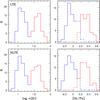 |
Fig. 4 Left panels: observed distribution of strontium abundances in logϵ(Sr). Right panels: histogram distribution of [Sr/Fe] for the stars colored in red and blue in the left histograms. Upper panels show the LTE Sr abundances, lower panels represent the abundances corrected for NLTE effects. |
Based on our selection, our sample is composed of 56 s-poor and 45 s-rich stars. The s-poor stars have logϵ(Sr) = 1.09 ± 0.02 and σ = 0.11 (⟨ [Sr/Fe] ⟩ = −0.06 ± 0.02), while the s-rich ones have logϵ(Sr) = 1.59 ± 0.02 and σ = 0.11 (⟨ [Sr/Fe] ⟩ = 0.29 ± 0.02). The difference in Sr abundances between the two selected groups is logϵ(Sr) = 0.40 ± 0.03. To compare this result with the ones in M11a, we define the difference in abundance ratio for two elements A and B between the s-rich and s-poor stars as  [A/B] ≡ [A/B]s-rich − [A/B]s-poor, we obtain [Sr/Fe] ≡ + 0.35 ± 0.03. This difference and the mean [Sr/Fe] values for s-rich and s-poor stars agree well with the ones of the other n-capture elements reported in M09 and M11a. Since in the M 22 RGB stars the additional content of n-capture elements develops from s-processes (M11a; Da Costa & Marino 2009; Roederer et al. 2011), the observed Sr increase in a group of SGB stars must also have a s-process origin.
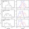 |
Fig. 5 Observed distribution of Ba in log(ϵ) abundances (left panels) and in abundance ratios relative to iron (right panels). The histogram distributions of [Ba/Fe] for s-rich and s-poor stars selected as in Fig. 4, have been represented in red and blue, respectively. The upper panels represent Ba abundances with Solar System (S.S.) isotopic ratios adopted for both s-rich and s-poor stars. In the middle panels, an r-only isotopic ratio has been applied for the s-poor stars. The lower panels represent the same abundances represented in the middle panels corrected for NLTE effects. |
4.2. Barium
In our previous work on RGB M 22 stars, we have found a bimodality in the Ba abundances (M09 and M11a). However, from our analysis of SGB stars, the various Ba abundance distributions shown in Fig. 5 fail to cleanly support the expected bimodality. This is likely due to the larger uncertainty introduced by the high sensitivity of the very strong Ba ii 4554 Å line to microturbulent velocity choices and to assumptions about r/s isotopic fractions, as discussed in Sect. 3.2. Here we just consider the isotopic dependence.
In the top panel of Fig. 5 we show the Ba abundances derived under assumption that the isotopic ratios are simply those of solar material. The s-poor and s-rich histograms show very little separation in [Ba/Fe]. In the middle panel we show a more realistic situation by showing LTE Ba abundances computed using a pure r isotopic ratio for s-poor stars. The mean Ba abundance of the s-poor stars decreases from logϵ(Ba) = 0.87 ± 0.02 (⟨ [Ba/Fe] ⟩ LTE = 0.24 ± 0.02, σ = 0.18) to logϵ(Ba) = 0.67 ± 0.02 (⟨ [Ba/Fe] ⟩ LTE = 0.04 ± 0.02, σ = 0.18). Finally, in the bottom panel we apply NLTE corrections to the abundances from the middle panel. Clearly there is still significant overlap in s-poor and s-rich distributions. However, considering only the NLTE Ba abundances, the mean value for the s-poor stars is logϵ(Ba) = 0.60 ± 0.02 (⟨ [Ba/Fe] ⟩ NLTE = −0.03 ± 0.02 (σ = 0.16). This value is very close to the one obtained for RGB stars by analyzing transitions in the yellow/red spectral regions, ⟨ [Ba/Fe] ⟩ = −0.05 ± 0.03 (Table 7 of M11a). The mean Ba content for s-rich stars, logϵ(Ba) = 1.10 ± 0.03 (⟨ [Ba/Fe] ⟩ NLTE = 0.32 ± 0.03, σ = 0.22), also agrees with the RGB value, ⟨ [Ba/Fe] ⟩ = 0.31 ± 0.04 (also Table 7 from M11a).
In comparing the Ba and Sr distributions in Figs. 4 and 5, the less precise results for Ba are apparent. The Ba dispersions for both s-rich and s-poor stars are much higher than the ones for Sr. But confidence in the basic results for Ba increases by plotting the individual Ba and Sr abundances. We show this in Fig. 6, where our selected s-rich and s-poor stars have been represented with different symbols in the [Sr/Fe]-[Ba/Fe] and in the [Sr/H]-[Ba/H] planes. These elements in the solar system are expected to be equally sensitive to s-process nucleosynthesis (see Table 10 in Simmerer et al. 2004). In M 22 they correlate closely on average. In conclusion, we confirm for SGB stars the s-process abundance bimodality found among the RGB stars in M09 and M11a.
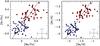 |
Fig. 6 [Sr/Fe] and [Sr/H] as a function of [Ba/Fe] and [Ba/H]. s-rich and s-poor stars are plotted in red circles and blue triangles, respectively. The dash-dotted line represents the perfect agreement. |
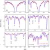 |
Fig. 7 Combined s-poor (blue) and s-rich (red) spectra constructed by averaging the spectra for eight s-poor stars (#2544, #2207, #2201, #2801, #1913, #735, #3, #768) and eight s-rich stars (#1924, #2659, #2153, #2414, #2404, #2099, #2607, #729) with similar atmospheric parameters. |
4.3. Carbon
Carbon abundances among RGB stars in M 22 have been determined by M11a. They found a wide spread in C content both among s-poor and s-rich stars, with the mean C abundance higher for s-rich stars by 0.35 ± 0.13. In addition, in each s-group C was found to be anticorrelated with N. This implies that in each s-group, separately, a subsample of stars is present that have undergone high-temperature H burning.
We find a wide spread of carbon also among the SGB stars. The s-rich stars have significantly larger mean carbon abundances than those of the s-poor stars: logϵ(C) = 6.99 ± 0.03 (⟨ [C/Fe] ⟩ = + 0.10 ± 0.03, σ = 0.23), while s-poor stars have logϵ(C) = 6.67 ± 0.02 (⟨ [C/Fe] ⟩ = −0.07 ± 0.03, σ = 0.19). Thus the abundance difference between the two groups is [C/Fe] = 0.17 ± 0.04, a more than 2σ difference, consistent with the difference found for RGB stars ([C/Fe] = 0.35 ± 0.13, M11a).
To visualize our results better, we computed an average-s-rich and an average-s-poor spectrum by combining stars with very similar atmospheric parameters. The comparison between the two averaged spectra around the spectral features of greatest interest is shown in Fig. 7. The s-rich spectrum clearly shows stronger Sr, Ba CH features with respect to the s-poor one. The two available H-lines, shown in the upper panels, show very similar wings, implying that our atmospheric parameters are reasonably correct and that the averaged stars have similar parameters.
The mean C abundance among RGB stars (M11a) is ~0.5 lower than among SGB stars. This is likely due to the decrease in [C/Fe] ratios around the RGB bump (MV ~ 0.5), and can be explained by the onset of a second mixing episode during the red-giant evolution of a population II star, once the molecular weight barrier established by the retreating convective envelope is wiped out by the advancing shell of H-burning (e.g. Sweigart & Mengel 1979; Charbonnel 1995). From that time onward, CN-processed material is able to reach the surface layer, where a decrease in C is visible.
We also see a trend in [C/Fe] with evolutionary phase, as shown in panels (a) and (b) of Fig. 8, where C abundances are plotted as a function of Teff. As a comparison, Sr abundances represented in panels (c) and (d) do not show any trend with Teff. For clarity, we binned abundances in intervals of 200 K in Teff and determined the mean [C/Fe] and [Sr/Fe] abundances for each bin for s-rich and s-poor stars individually, and for the total sample. To these mean abundances for each bin, we associated the error bars corresponding to the σ divided by  , with N being the number of measurements per bin. Error bars in the righthand corner of panels (a) and (c) represent the σ values for the s-rich, s-poor, and for the entire sample.
The carbon rise is particularly pronounced for Teff > 6000 K. The reason for this trend is not clear. For stars with Teff > 6000 K the uncertainties associated to the C abundances are surely higher due to the lower line strengths, and reach values of ~0.20–0.25. These uncertainties could have led to a systematic overestimation of C for the hotter stars. The C rise could also likely come from our 1D approximation for model atmospheres. A more appropriate analysis of molecular bands should consider 3D effects that strongly depend on temperature (Collet et al. 2007). However, since this effect does not appear to be significantly different between s-rich and s-poor stars, it does not affect our differential abundance analysis between s-rich and s-poor stars in M 22.
We have already established that the mean value of [C/Fe] is substantially higher for the s-rich stars than for the s-poor stars over the entire range of SGB Teff. In Fig. 9 the C distribution is represented for the s-poor stars (upper panel) and s-rich stars (lower panel). The distribution of carbon for the two groups of stars suggests there is an intrinsic dispersion in C among both s-rich and s-poor stars. Indeed, both show intrinsic variations of C, N, O, and Na with the presence of N-C and Na-O anticorrelations, as revealed in our high-resolution spectroscopic study of RGBs (M11a). The [C/Fe] abundance dispersion for the s-rich and the s-poor groups here (σ is 0.23 and 0.19 dex, respectively) are marginally larger than the measurement error, which is typically 0.15 dex, and indicate the presence of an intrinsic [C/Fe] spread.
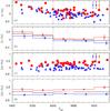 |
Fig. 8 C and Sr abundance ratios relative to Fe as a function of Teff. In panels a) and c), s-poor and s-rich stars are represented by blue triangles and red circles, respectively. The observed dispersions for s-poor (blue), s-rich (red), and the total sample of stars (black) are also shown. In panels b) and d) we plot the mean [C/Fe] and [Sr/Fe] values in intervals of 200 K in Teff, with associated errors, for the two s groups (red and blue lines), and for the total sample (black line). |
5. The double sub-giant branch of M 22
M 22 is among the GCs showing a double SGB (Piotto 2009, 2012; M09). In the cluster center the bright SGB component is made up of about 65% of SGB stars while the remaining ~35% of stars defines the fainter SGB component. The multi-wavelength study of M 22 from Piotto et al. (2012) reveals that the SGB bimodality is visible in all the bands, from the far ultraviolet (the F275W HST/WFC3 filter) up to the near infrared (the F814W HST/WFC3 filter). These authors also found that the average magnitude difference between the bright SGB and the faint SGB is almost the same at different wavelengths, suggesting that the split reflects internal structural properties of the stars, and not only the surface composition.
The RGB of M 22 is also made up of two main components, but the RGB split is only visible when appropriate photometric bands are used, such as m1 and the hk Strömgren indices (Richter et al. 1999; Lee et al. 2009) or the U band (see Fig. 1). While the SGB split is consistent with two stellar groups with either an age difference of ~1–2 Gyr, or a difference in their overall C+N+O content, the occurrence of simultaneous RGB and SGB bimodality observed in the U − V color seems to rule out the first hypothesis of a significant age difference (as suggested by Sbordone et al. 2011, for the case of NGC 1851).
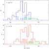 |
Fig. 9 Carbon abundance relative to Fe distributions for the s-poor (upper panel) and s-rich (lower panel) stars. In each panel the dashed line represents the mean [C/Fe] abundance. The location of the stars selected for constructing the average s-rich and s-poor spectrum (see Fig. 7) has been indicated with dashed red and blue histograms, respectively. The dashed green histogram represents the location of stars with Teff > 6000 K, showing a rise in C with temperature. |
M11a have shown that the blue and the red RGB sequences appearing in the I versus m1 diagram in lefthand panel of Fig. 10 are made of s-poor (iron/CNO-poor) and s-rich (iron/CNO-rich) stars, respectively. This CMD is a reproduction of the same I versus m1 diagram of Fig. 19 in M11a, but now we have color-coded the stars photometrically belonging to the two RGBs. The same color codes are used to plot these selected stars in common with the SUSI photometry, represented in the U-(U − V) CMD (right panel of Fig. 10). In the latter CMD the two RGBs are clearly connected to the two SGBs, providing photometric evidence that the bright SGB and the faint SGB are the sub-giant counterparts of the s-poor and s-rich RGB, respectively.
Here we can provide direct evidence of the RGBs-SGBs connection, already clear from the CMD inspection, by matching our spectroscopic data on M 22 SGB stars with the CMDs where the split is more clearly visible. We remind the reader that our photometry has been corrected for differential reddening effects by applying the procedure described in Milone et al. (2012, see Sect. 2).
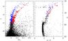 |
Fig. 10 Left panel: I versus the Strömgren index m1 diagram. Stars belonging to the two RGBs are represented in red and blue colors. Right panel: Stars selected in the double RGB of the I-m1 diagram are represented in the U-(U − V) CMD. |
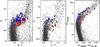 |
Fig. 11 M 22 double SGB in B-(B − V), U-(U − V), and in the mF606W-(mF606W − mF814W) CMDs, with the s-rich and s-poor stars superimposed. |
The ground-based and HST CMDs are shown in Fig. 11, with our s-rich and s-poor stars superimposed. The lefthand panel shows a ground-based B-(B − V) CMD for stars distributed in a large field (34′ × 33′) of M 22 where we have plotted relatively isolated, unsaturated stars with accurate values of the PSF-fitting quality index and small σ errors in photometry and astrometry (see Sect. 2.1). The U-(U − V) CMD in the middle panel is from SUSI2 ground-based photometry, but it covers a small field (two chips of 2.7′ × 5.5′) on the outskirts of the cluster. The righthand panel contains the ACS/HST CMD representing stars lying in the most central field (3′ × 3′) of the cluster. The double SGB of M 22 is clear in all these photometric systems. By coupling our spectroscpic results with these CMDs, it turns out that the s-rich stars occupy the fainter SGB, while the s-poor ones lie on the upper brighter SGB. All the CMDs of Fig. 11 suggest the same: the s-rich and s-poor stars segregate along two different branches on the M 22 SGB, as predicted by M09. The fact that both the fainter SGB and the redder RGB are made of s-rich stars, while s-poor stars are located on the brighter SGB and the bluer RGB, further confirms the connection between the two RGBs and SGBs.
Our results suggest that (i) the two SGBs are populated by stars with different s-process element content; (ii) the two SGBs evolve to the two sequences on the RGB observed in various M 22 CMDs and populated by stars with different s-process elements, overall metallicity, overall C+N+O, and slightly different Ca, as demonstrated in M11a. Unfortunately, given the moderate resolution of our SGB spectra, we cannot distinguish the small differences in [Fe/H] and [Ca/Fe] for SGBs stars between s-rich and s-poor stars as found from high-resolution spectroscopy on RGB. As found for RGB stars, the SGB s-rich and s-poor stars have slightly different C abundances, but we have no information on N and O for SGB stars. However, given that we have demonstrated that the two SGBs, in the same way as the two RGBs, have different s-process content and C, and that the sequences are photometrically linked, we can fairly extend the results on the two RGBs to the two SGBs for those elements not studied in the present work.
In the light of our results and previous results on the RGB stars by M09 and M11a, we can, for the first time, fully characterize the two SGBs of M 22 in terms of chemical composition, as follows:
-
faint-SGB: s-rich stars, with higher metallicity, Ca and enhanced C+N+O abundance;
-
bright-SGB: s-poor stars, with lower metallicity, Ca and unenhanced C+N+O abundance.
The chemical properties for the two SGBs are summarized in Table 4. For the present discussion we consider calcium and the C+N+O sum as part of the overall metallicity. Thus we take those values determined from RGB high-resolution spectroscopy in M11a, and extend them to the two SGBs with different s-process contents. As discussed in Sect. 4.3, elements like C are highly affected by evolutionary effects that change the surface abundances for stars at different evolutionary stages, but the total C+N+O is not affected by these effects.
Chemical features of the two M 22 SGBs.
Theoretical isochrones can reproduce SGB sequences with different luminosities by assuming an age difference among the two SGB populations. In this scenario, in M 22 the fainter-SGB would be populated by younger stars and the brighter SGB by older ones. If age is assumed to be the lone factor responsible for the M 22 SGB split, our isochrones can reproduce the observed separation in magnitude with an age difference of ~1 Gyr between the two SGB populations. Of course, this is only true in the case of two stellar populations with identical chemical properties.
However, our results show that there are chemical differences among the two SGBs, so that the scenario of a simple age difference cannot work for this cluster. In particular, the overall C+N+O abundance has a strong impact on isochrones at SGB luminosities. This has fundamental consequences for GC age dating, as demonstrated in recent literature by Cassisi et al. (2008) and D’Antona et al. (2009). For NGC 1851, Cassisi et al. (2008) and Ventura et al. (2009) suggested that the fainter SGB stars could be younger by a few hundred Myrs, if enhanced in the total C+N+O content. Following this scenario large age differences among the two SGBs could be ruled out.
In M 22 the SGB s-rich stars are distributed along the faint SGB, indicating that the faint SGB is composed of stars enriched in s-process elements, and additionally in the total CNO and metallicity, as suggested by our previous study on RGB stars. Here, we use isochrones interpolated in the BASTI database7 with the exact CNO and metallicity (determined in our previous work and listed in Table 4), to investigate the relative age difference among the s-rich and s-poor stars. As demonstrated by M09 (see their Fig. 19), isochrones at the same age, and with metallicity different by 0.15 dex (as observed from high-resolution spectra), cannot reproduce the entire size of the split. The isochrone fitting accounting for both the metallicity and CNO variation to the SGB region is shown in Fig. 12 for the mF606W versus mF606W − mF814W CMD. The middle blue and red tracks represent the best fitting isochrones to the brighter and the fainter SGB respectively. The age was assumed equal to 13.5 Gyr, which is the value for which the models give the best fit to the data. For each of the best-fitting tracks we also show isochrones with the same chemistry but with the age varied by ± 300 Myr, which is the typical error affecting the determination of relative ages from isochrone fitting. It is clear that, by taking the observed difference in the CNO total content into account, the size of the SGB split is consistent with isochrones of the same age. A possible He variation (if any) in this range of metallicity and ages is not expected to change the separation in luminosity between the two SGBs, but only modify the SGB shape (Ventura et al. 2009). From this analysis, the s-rich stars appear to be coeval (or possibly slightly younger) to the s-poor stars, indicating that star formation in M 22 could have developed very rapidly. Possible age differences smaller than ~300 Myr cannot be distinguished by our results.
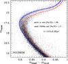 |
Fig. 12 Isochrones computed with the observed CNO and metallicity of the two s groups and the same age (13.5 Gyr) superimposed on the M 22 SGBs. The red and blue central tracks are the CNO-higher (s-rich) and CNO-lower (s-poor) best-fitting isochrones, respectively. For both we computed a couple of isochrones with the same chemistry, but with age varying of ± 300 Myr. |
6. Formation scenarios
In the attempt to understand the chemical and photometric observations in M 22, two different scenarios can basically be explored, depending on how different bursts of star formation could have occurred, spatially or temporally separated.
In the first case we may “simply” assume that star formation bursts occurred in separated regions that eventually merged together. Then, the s-poor and s-rich stars could have been formed out of interstellar mediums with slightly different metallicities, and with differences in the total C+N+O and s-process elements.
If instead, the different bursts of star formation have occurred at different epochs of the cluster evolution, multiple stellar populations in M 22 are assumed to be the result of self-pollution, with the s-rich (metal-richer) stars the younger population, since they show signatures of pollution from neutron-capture material. As far as we know, the self-pollution hypothesis in M 22 would require a number of complex and “fine-tuned” assumptions to reconcile the stellar yields and the lifetimes of possible polluters with the observations (see Sect. 6.1 for more details). In this scenario, any attempt to identify the responsible polluters should take the rapid evolution of the cluster into account, which we argued on the basis of observational spectroscopic and photometric results coupled with theoretical isochrones.
6.1. Chemical enrichment
Favorable nucleosynthetic sites for the s-process production are AGB stars with M ≲ 3–4 M⊙, which are predicted to experience multiple third dredge-up events (TDU). The number of TDUs decreases for lower mass AGB stars until a minimum mass for which the conditions for the activation of the TDU are never reached. This minimum mass is an increasing function of metallicity (e.g., Straniero et al. 2003). AGB stars more massive than 3–4 M⊙ do not experience many third dredge-up events. They are predicted to pollute the intracluster medium only in the p-capture products and, for this reason, have been proposed as candidate polluters responsible for the light-element (anti)correlations typical of GCs (D’Antona & Caloi 2004). The evolutionary timescale of the less massive AGBs (some hundreds of Myrs; see Table 1 in Ventura et al. 2009), may be consistent with the uncertainty associated to the zero age difference obtained from our isochrones constructed with different CNO contents. However, this still leaves problems in completely accounting for the chemical enrichment history of M 22.
A primary difficulty is the bimodal metallicity distribution of M 22, with the s-rich stars having higher Fe abundances (M09). This suggests that M 22 has also undergone enrichment in metallicity, so has been likely polluted by yields from Supernovae Type II (SN II, M09).
Moreover, in M 22 each s-group individually defines a Na-O anticorrelation, suggesting that both have suffered further enrichment from other polluters, e.g., intermediate-mass AGBs, fast-rotating massive stars, and/or massive binaries. Each of the two M 22 s-groups shows its own second-generation enriched in Na and depleted in O (see Fig. 14 in M11a), just like the patterns seen in all the GCs studied so far with sufficient statistics (e.g. Ramírez & Cohen 2002; Carretta et al. 2009). This chemical pattern is difficult to understand. We may speculate that the first stars to form after the first population of metal-poor, s-poor-poor, and Na-poor stars could have been the more metal-rich and s-rich Na-poor stars, as tentatively suggested by Marino et al. (2012) to interpret observations in ω Cen. These two populations could form their own Na-O anticorrelation at later times. A similar scenario would require efficient star formation and consuming of the available intracluster material to prevent each stellar burst being contaminated by the preceding one.
A chemical pattern similar to the one observed in M 22 is seen in ω Cen, even if much more complex (Johnson & Pilachowski 2010; Marino et al. 2011b; see Sect. 1 for more details). For this most peculiar GC, D’Antona et al. (2011) compared the Na and O abundances with theoretical AGB yields to account for the presence of the Na-O anticorrelation at different metallicities. They envisaged a chemical evolutionary scenario in which the high mass of ω Cen meant that the material ejected by SN II could survive in a torus that collapses back onto the cluster after the SN II epoch (see also D’Ercole et al. 2008). The 3D hydro simulations by Marcolini et al. (2006) in fact show that the collapse back includes the matter enriched by the SN II ejecta. A similar scenario could be tentatively extended to M 22.
Alternatively, because observations in GCs strongly suggest that the increase in s-process elements is linked to an increase in Fe, it would be tempting to speculate that s-process elements and Fe may have been produced by the same polluters. Indeed, as outlined in D’Antona et al. (2011), there are other possible sites of s-nucleosynthesis that have not been explored well at present, e.g. the carbon-burning shells of lower-mass progenitors of SN II (e.g., The et al. 2007). The pollution from these objects may become peculiarly apparent in the evolution of the progenitor systems of ω Cen and M 22.
Interestingly, Roederer et al. (2011) note that the s-process abundances in the s-rich stars could be more consistent with predictions for more massive AGB stars, those capable of activating the 22Ne(α, n)25 Mg reaction. The main difficulty with this scenario is the lack of a correlation between s-process enrichment and Na within the two groups, which would be expected if these elements are all produced by the same AGB stars of higher masses. However, stars with initial masses >3 M⊙ will evolve in ≲ 300 Myr, which would agree with our derived upper limit on the age difference of the two SGBs in M 22. We note here that the efficiency of s-processes depends not only on the number of neutrons but also on the neutron-to-seed nuclei (most likely Fe) ratio. However, the lack of complete grids of theoretical yields for various masses at the exact metallicity of M 22 (Cristallo et al. 2011) makes it difficult to draw definitive conclusions about the mass of the AGB polluters, in the hypothesis that AGBs are effectively the producers of the extra s-material in M 22 s-rich stars. More generally, we admit that the proposed self-pollution channels require an uncomfortable level of fine-tunings. The uncertainties, and in some cases the lack, of predicted theoretical yields from different kinds of polluters, introduces further difficulties in interpreting data in the self-pollution framework.
Some of the difficulties encountered by the self-pollution scenario may be overcome by invoking a spatial separation (instead of a temporal one) for the different bursts of star formation in a merger scenario. Very recently, dynamical simulations by Bekki & Yong (2012) have shown that it is dynamically plausible that two GCs merge and form a new GC in the central region of its host dwarf galaxy. The host dwarf galaxy is cannibalized through tidal interactions with the Milky Way, and only the compact nucleus survives as a present-day AGC. This scenario has the advantage of explaining the chemical features of the two s-groups of stars in M 22 in a simple manner (e.g., their different metallicity and s-process elements content, and the presence of an individual Na-O anticorrelation). However, one still has to understand why the multiple stellar population phenomenon looks similar in all the AGCs investigated so far. As an example, in both M 22 and NGC 1851, the s-rich stars are slightly enriched in metallicity. In addition if we consider M 22 and ω Cen, the metal-richer and s-richer stars populate fainter SGBs in both of those clusters. The occurrence of these similarities may be more easily understood in a self-enrichment scenario. However, for completeness we note the distribution of s-rich and s-poor stars on the SGBs of NGC 1851 could be inverted with respect to M 22, as suggested by Carretta et al. (2011), but no direct observations of SGB are currently available for this GC.
At present we are unable to provide a definitive and clear explanation for the M 22’s formation and evolution. Both the self-enrichment and the merger scenarios have pros and cons. We only note here that they represent a very different way to interpret M 22 and other AGCs. In the first hypothesis, they could be similar to normal clusters, but the star formation could have occurred further and/or, owing to their initial higher masses, could have retained material that escaped from normal GCs. In the second hypothesis, the AGCs may have been formed through different mechanisms (i.e. a merger) in exceptional conditions, most probably in extragalactic environments.
7. Conclusion
We have presented a medium-resolution spectroscopic analysis of a hundred SGB stars in the double-SGB GC M 22. The faint SGB is populated by s-rich (metal-rich) stars, and the bright SGB by s-poor (metal-poor) stars. Our abundance analysis constitutes the first direct evidence of a connection between the two RGBs populated by the two s-process stellar groups, as discovered in our previous work, and the double SGB. This SGBs-RGBs connection was also confirmed by inspecting the U-(U − V) CMD: the fainter SGB population clearly evolves in a redder RGB sequence populated by s-rich stars, and the brighter SGB in a bluer branch populated instead by the s-poor stars (M11a). Among the RGB stars studied by M11a, the s-rich stars are also enhanced in the total CNO with respect to the s-poor ones. We can at least extend their conclusions about the total CNO to the present SGB sample.
Isochrones constructed with our observed metallicities and C+N+O content for the two s groups observed on the RGB suggest that the split SGB is consistent with the two stellar groups being coeval within an uncertainty of ~300 Myr.
Based on our observations, we discussed possible evolutionary histories for the cluster, both in a self-enrichment and in a merger scenario. We underline the difficulties that both scenarios have to overcome and encourage further investigations into both the theoretical and observational sides to finally shed light on the nature of the Milky Way AGCs.
Online material
M 22 targets: positions and photometric data.
M 22 C, Sr, Ba abundances for SGB stars, listing standard deviation σSr for the two Sr lines and the s-group for each star.
The 2010 updated version of the Harris catalog is available at http://www.physics.mcmaster.ca/~harris/mwgc.dat
See http://www.phys.appstate.edu/spectrum/spectrum.html for more details.
Available at http://www.as.utexas.edu/~chris/moog.html
Acknowledgments
We thank F. D’Antona, R. Gratton, and C. Allende Prieto for useful comments on the manuscript, and the anonymous referee for his/her suggestions. A.P.M., G.P., S.C., and A.A. are funded by the Ministry of Science and Technology of the Kingdom of Spain (grant AYA 2010-16717). A.P.M. and A.A. are also funded by the Instituto de Astrofŋsica de Canarias (grant P3-94). I.U.R. is supported by the Carnegie Institution of Washington through the Carnegie Observatories Fellowship. C.S. is funded by US National Science Foundation grant AST-0908978. M.Z. acknowledges the FONDAP Center for Astrophysics 15010003, the BASAL CATA PFB-06, the Milky Way Millennium Nucleus from the Ministry of Economics ICM grant P07-021-F, Proyecto FONDECYT Regular 1110393, and Proyecto Anillo ACT-86 CS.
References
- Alonso, A., Arribas, S., & Martinez-Roger, C. 1999, A&A, 140, 261 [Google Scholar]
- Anderson, J., & King, I. R. 2006, Instrument Science Report ACS 2006-01, 34, 1 [Google Scholar]
- Anderson, J., Sarajedini, A., Bedin, L. R., et al. 2008, AJ, 135, 2055 [NASA ADS] [CrossRef] [Google Scholar]
- Arlandini, C., Käppeler, F., Wisshak, K., et al. 1999, ApJ, 525, 886 [NASA ADS] [CrossRef] [Google Scholar]
- Bekki, K., & Norris, J. E. 2006, ApJ, 637, L109 [NASA ADS] [CrossRef] [Google Scholar]
- Bekki, K., & Yong, D. 2012, MNRAS, 419, 2063 [NASA ADS] [CrossRef] [Google Scholar]
- Bellini, A., Bedin, L. R., Piotto, G., et al. 2010, AJ, 140, 631 [NASA ADS] [CrossRef] [Google Scholar]
- Bergemann, M., & Gehren, T. 2008, A&A, 492, 823 [NASA ADS] [CrossRef] [EDP Sciences] [Google Scholar]
- Carretta, E., Bragaglia, A., Gratton, R. G., et al. 2009, A&A, 505, 117 [NASA ADS] [CrossRef] [EDP Sciences] [Google Scholar]
- Carretta, E., Gratton, R. G., Lucatello, S., et al. 2010, ApJ, 722, L1 [NASA ADS] [CrossRef] [Google Scholar]
- Carretta, E., Lucatello, S., Gratton, R. G., Bragaglia, A., & D’Orazi, V. 2011, A&A, 533, A69 [NASA ADS] [CrossRef] [EDP Sciences] [Google Scholar]
- Casagrande, L., Ramírez, I., Meléndez, J., Bessell, M., & Asplund, M. 2010, A&A, 512, A54 [NASA ADS] [CrossRef] [EDP Sciences] [Google Scholar]
- Cassisi, S., Salaris, M., Pietrinferni, A., et al. 2008, ApJ, 672, L115 [NASA ADS] [CrossRef] [Google Scholar]
- Castelli, F., & Kurucz, R. L. 2004 [arXiv:astro-ph/0405087] [Google Scholar]
- Charbonnel, C. 1995, ApJ, 453, L41 [NASA ADS] [CrossRef] [Google Scholar]
- Clampin, M., Sirianni, M., Hartig, G. F., et al. 2002, Exper. Astron., 14, 107 [NASA ADS] [CrossRef] [Google Scholar]
- Cohen, J. G., Kirby, E. N., Simon, J. D., & Geha, M. 2010, ApJ, 725, 288 [NASA ADS] [CrossRef] [Google Scholar]
- Collet, R., Asplund, M., & Trampedach, R. 2007, A&A, 469, 687 [NASA ADS] [CrossRef] [EDP Sciences] [Google Scholar]
- Collet, R., Asplund, M., & Nissen, P. E. 2009, PASA, 26, 330 [NASA ADS] [CrossRef] [Google Scholar]
- Cristallo, S., Piersanti, L., Straniero, O., et al. 2011, ApJS, 197, 17 [NASA ADS] [CrossRef] [Google Scholar]
- Da Costa, G. S., & Marino, A. F. 2011, PASA, 28, 28 [NASA ADS] [Google Scholar]
- Da Costa, G. S., Held, E. V., Saviane, I., & Gullieuszik, M. 2009, ApJ, 705, 1481 [NASA ADS] [CrossRef] [Google Scholar]
- D’Antona, F., & Caloi, V. 2004, ApJ, 611, 871 [NASA ADS] [CrossRef] [Google Scholar]
- D’Antona, F., Stetson, P. B., Ventura, P., et al. 2009, MNRAS, 399, L151 [NASA ADS] [Google Scholar]
- D’Antona, F., D’Ercole, A., Marino, A. F., et al. 2011, ApJ, 736, 5 [NASA ADS] [CrossRef] [Google Scholar]
- Decressin, T., Meynet, G., Charbonnel, C., Prantzos, N., & Ekström, S. 2007, A&A, 464, 1029 [NASA ADS] [CrossRef] [EDP Sciences] [Google Scholar]
- de Mink, S. E., Pols, O. R., Langer, N., & Izzard, R. G. 2009, A&A, 507, L1 [NASA ADS] [CrossRef] [EDP Sciences] [Google Scholar]
- D’Ercole, A., Vesperini, E., D’Antona, F., McMillan, S. L. W., & Recchi, S. 2008, MNRAS, 391, 825 [NASA ADS] [CrossRef] [Google Scholar]
- Dickens, R. J., & Woolley, R. v. d. R. 1967, Royal Greenwich Observatory Bulletins, 128, 255 [NASA ADS] [Google Scholar]
- Ferraro, F. R., Dalessandro, E., Mucciarelli, A., et al. 2009, Nature, 462, 483 [NASA ADS] [CrossRef] [PubMed] [Google Scholar]
- Freeman, K. C., & Rodgers, A. W. 1975, ApJ, 201, L71 [NASA ADS] [CrossRef] [Google Scholar]
- Gallagher, A. J., Ryan, S. G., García Pérez, A. E., & Aoki, W. 2010, A&A, 523, A24 [NASA ADS] [CrossRef] [EDP Sciences] [Google Scholar]
- Gratton, R. G., Carretta, E., & Castelli, F. 1996, A&A, 314, 191 [NASA ADS] [Google Scholar]
- Gratton, R., Sneden, C., & Carretta, E. 2004, ARA&A, 42, 385 [NASA ADS] [CrossRef] [Google Scholar]
- Gray, R. O., & Corbally, C. J. 1994, AJ, 107, 742 [NASA ADS] [CrossRef] [Google Scholar]
- Harris, W. E. 1996, AJ, 112, 1487 [NASA ADS] [CrossRef] [Google Scholar]
- Hill, V., Plez, B., Cayrel, R., et al. 2002, A&A, 387, 560 [NASA ADS] [CrossRef] [EDP Sciences] [Google Scholar]
- Johnson, C. I., & Pilachowski, C. A. 2010, ApJ, 722, 1373 [NASA ADS] [CrossRef] [Google Scholar]
- Kappeler, F., Beer, H., & Wisshak, K. 1989, Rep. Prog. Phys., 52, 945 [Google Scholar]
- Kraft, R. P. 1994, PASP, 106, 553 [NASA ADS] [CrossRef] [Google Scholar]
- Kurucz, R. L. 1992, The Stellar Populations of Galaxies (Dordrecht: Kluwer), IAU Symp., 149, 225 [NASA ADS] [CrossRef] [Google Scholar]
- Lee, J.-W., Kang, Y.-W., Lee, J., & Lee, Y.-W. 2009, Nature, 462, 480 [NASA ADS] [CrossRef] [PubMed] [Google Scholar]
- Lodders, K. 2003, ApJ, 591, 1220 [NASA ADS] [CrossRef] [Google Scholar]
- Mandushev, G., Staneva, A., & Spasova, N. 1991, A&A, 252, 94 [NASA ADS] [Google Scholar]
- Marcolini, A., D’Ercole, A., Brighenti, F., & Recchi, S. 2006, MNRAS, 371, 643 [NASA ADS] [CrossRef] [Google Scholar]
- Marino, A. F., Villanova, S., Piotto, G., et al. 2008, A&A, 490, 625 [NASA ADS] [CrossRef] [EDP Sciences] [Google Scholar]
- Marino, A. F., Milone, A. P., Piotto, G., et al. 2009, A&A, 505, 1099 [NASA ADS] [CrossRef] [EDP Sciences] [Google Scholar]
- Marino, A. F., Sneden, C., Kraft, R. P., et al. 2011a, A&A, 532, A8 [NASA ADS] [CrossRef] [EDP Sciences] [Google Scholar]
- Marino, A. F., Milone, A. P., Piotto, G., et al. 2011b, ApJ, 731, 64 [NASA ADS] [CrossRef] [Google Scholar]
- Marino, A. F., Milone, A. P., Piotto, G., et al. 2012, ApJ, 746, 14 [NASA ADS] [CrossRef] [Google Scholar]
- Mashonkina, L., & Zhao, G. 2006, A&A, 456, 313 [NASA ADS] [CrossRef] [EDP Sciences] [Google Scholar]
- Milone, A. P., Bedin, L. R., Piotto, G., et al. 2008, ApJ, 673, 241 [NASA ADS] [CrossRef] [Google Scholar]
- Milone, A. P., Stetson, P. B., Piotto, G., et al. 2009, A&A, 503, 755 [NASA ADS] [CrossRef] [EDP Sciences] [Google Scholar]
- Milone, A. P., Piotto, G., Bedin, L. R., et al. 2012, A&A, 537, A77 [NASA ADS] [CrossRef] [EDP Sciences] [Google Scholar]
- Momany, Y., Bedin, L. R., Cassisi, S., et al. 2004, A&A, 420, 605 [NASA ADS] [CrossRef] [EDP Sciences] [Google Scholar]
- Norris, J. E., & DaCosta, G. S. 1995, ApJ, 447, 680 [NASA ADS] [CrossRef] [Google Scholar]
- Pasquini, L., Avila, G., Blecha, A., et al. 2002, The Messenger, 110, 1 [NASA ADS] [Google Scholar]
- Pasquini, L., Alonso, J., Avila, G., et al. 2003, Proc. SPIE, 4841, 1682 [NASA ADS] [CrossRef] [Google Scholar]
- Peterson, R. C., & Cudworth, K. M. 1994, ApJ, 420, 612 [NASA ADS] [CrossRef] [Google Scholar]
- Piotto, G. 2009, IAU Symp., 258, 233 [NASA ADS] [Google Scholar]
- Piotto, G., & Milone, A. P., Bedin, L. R., et al. 2012, ApJ, submitted [Google Scholar]
- Ramírez, S. V., & Cohen, J. G. 2002, AJ, 123, 3277 [NASA ADS] [CrossRef] [MathSciNet] [Google Scholar]
- Richter, P., Hilker, M., & Richtler, T. 1999, A&A, 350, 476 [NASA ADS] [Google Scholar]
- Roederer, I. U., Marino, A. F., & Sneden, C. 2011, ApJ, 742, 37 [Google Scholar]
- Sbordone, L., Salaris, M., Weiss, A., & Cassisi, S. 2011, A&A, 534, A9 [NASA ADS] [CrossRef] [EDP Sciences] [Google Scholar]
- Short, C. I., & Hauschildt, P. H. 2006, ApJ, 641, 494 [NASA ADS] [CrossRef] [Google Scholar]
- Simmerer, J., Sneden, C., Cowan, J. J., et al. 2004, ApJ, 617, 1091 [NASA ADS] [CrossRef] [Google Scholar]
- Sirianni, M., Jee, M. J., Benítez, N., et al. 2005, PASP, 117, 1049 [NASA ADS] [CrossRef] [Google Scholar]
- Sneden, C. 1973, ApJ, 184, 839 [NASA ADS] [CrossRef] [Google Scholar]
- Sollima, A., Ferraro, F. R., Pancino, E., & Bellazzini, M. 2005, MNRAS, 357, 265 [NASA ADS] [CrossRef] [Google Scholar]
- Stetson, P. B. 2000, PASP, 112, 925 [NASA ADS] [CrossRef] [Google Scholar]
- Stetson, P. B. 2005, PASP, 117, 563 [CrossRef] [Google Scholar]
- Straniero, O., Domínguez, I., Cristallo, S., & Gallino, R. 2003, PASA, 20, 389 [NASA ADS] [CrossRef] [Google Scholar]
- Suntzeff, N. B., & Kraft, R. P. 1996, AJ, 111, 1913 [NASA ADS] [CrossRef] [Google Scholar]
- Sweigart, A. V., & Mengel, J. G. 1979, ApJ, 229, 624 [NASA ADS] [CrossRef] [Google Scholar]
- The, L.-S., El Eid, M. F., & Meyer, B. S. 2007, ApJ, 655, 1058 [NASA ADS] [CrossRef] [Google Scholar]
- Vanbeveren, D., Mennekens, N., & De Greve, J. P. 2011 [arXiv:1109.2713] [Google Scholar]
- Ventura, P., D’Antona, F., Mazzitelli, I., & Gratton, R. 2001, ApJ, 550, L65 [NASA ADS] [CrossRef] [Google Scholar]
- Ventura, P., Caloi, V., D’Antona, F., et al. 2009, MNRAS, 399, 934 [NASA ADS] [CrossRef] [Google Scholar]
- Yong, D., & Grundahl, F. 2008, ApJ, 672, L29 [NASA ADS] [CrossRef] [Google Scholar]
- Yong, D., Grundahl, F., Johnson, J. A., & Asplund, M. 2008, ApJ, 684, 1159 [NASA ADS] [CrossRef] [Google Scholar]
- Yong, D., Grundahl, F., D’Antona, F., et al. 2009, ApJ, 695, L62 [NASA ADS] [CrossRef] [Google Scholar]
All Tables
M 22 C, Sr, Ba abundances for SGB stars, listing standard deviation σSr for the two Sr lines and the s-group for each star.
All Figures
|
Fig. 1 Comparison of the U versus (U − V) CMD from NTT photometry (Momany et al. 2004) before (panel a)) and after (panel b)) the correction for differential (but not for the absolute) reddening. The horizontal branch stars lie at U ~ 17. The Δ(U − V) distributions of RGB stars with respect to the fiducial (red dash-dotted line on the CMDs) are shown in panels c) and d) for the uncorrected CMD, and in panels g) and h) for the corrected one. For SGB stars we show the distributions of the ΔU magnitude relative to the fiducial shown in the CMDs for the uncorrected (panels e) and f)) and the corrected (panels i) and l)) CMDs. |
| In the text | |
|
Fig. 2 Fe i lines for the combined s-poor (lower) and s-rich (upper) spectra of Fig. 7. Superimposed on the observed spectra are synthetic spectra corresponding to the [Fe/H] = −1.67 (red), [Fe/H] = −1.82 (blue), and with no Fe (magenta). |
| In the text | |
|
Fig. 3 Observed and synthetic spectra around the Sr lines at 4077 Å and 4215 Å and the G band for the s-rich star #2505. In each panel the points represent the observed spectrum, and the continuous lines are the synthesis computed with different strontium and carbon abundances. The magenta line is the spectrum computed with no contribution from Sr ii and C; the red line is the best-fitting synthesis (with the abundances given in Table 3); and the green and blue lines are the syntheses computed with Sr and C abundances altered by ± 0.3 dex from the best value. |
| In the text | |
|
Fig. 4 Left panels: observed distribution of strontium abundances in logϵ(Sr). Right panels: histogram distribution of [Sr/Fe] for the stars colored in red and blue in the left histograms. Upper panels show the LTE Sr abundances, lower panels represent the abundances corrected for NLTE effects. |
| In the text | |
|
Fig. 5 Observed distribution of Ba in log(ϵ) abundances (left panels) and in abundance ratios relative to iron (right panels). The histogram distributions of [Ba/Fe] for s-rich and s-poor stars selected as in Fig. 4, have been represented in red and blue, respectively. The upper panels represent Ba abundances with Solar System (S.S.) isotopic ratios adopted for both s-rich and s-poor stars. In the middle panels, an r-only isotopic ratio has been applied for the s-poor stars. The lower panels represent the same abundances represented in the middle panels corrected for NLTE effects. |
| In the text | |
|
Fig. 6 [Sr/Fe] and [Sr/H] as a function of [Ba/Fe] and [Ba/H]. s-rich and s-poor stars are plotted in red circles and blue triangles, respectively. The dash-dotted line represents the perfect agreement. |
| In the text | |
|
Fig. 7 Combined s-poor (blue) and s-rich (red) spectra constructed by averaging the spectra for eight s-poor stars (#2544, #2207, #2201, #2801, #1913, #735, #3, #768) and eight s-rich stars (#1924, #2659, #2153, #2414, #2404, #2099, #2607, #729) with similar atmospheric parameters. |
| In the text | |
|
Fig. 8 C and Sr abundance ratios relative to Fe as a function of Teff. In panels a) and c), s-poor and s-rich stars are represented by blue triangles and red circles, respectively. The observed dispersions for s-poor (blue), s-rich (red), and the total sample of stars (black) are also shown. In panels b) and d) we plot the mean [C/Fe] and [Sr/Fe] values in intervals of 200 K in Teff, with associated errors, for the two s groups (red and blue lines), and for the total sample (black line). |
| In the text | |
|
Fig. 9 Carbon abundance relative to Fe distributions for the s-poor (upper panel) and s-rich (lower panel) stars. In each panel the dashed line represents the mean [C/Fe] abundance. The location of the stars selected for constructing the average s-rich and s-poor spectrum (see Fig. 7) has been indicated with dashed red and blue histograms, respectively. The dashed green histogram represents the location of stars with Teff > 6000 K, showing a rise in C with temperature. |
| In the text | |
|
Fig. 10 Left panel: I versus the Strömgren index m1 diagram. Stars belonging to the two RGBs are represented in red and blue colors. Right panel: Stars selected in the double RGB of the I-m1 diagram are represented in the U-(U − V) CMD. |
| In the text | |
|
Fig. 11 M 22 double SGB in B-(B − V), U-(U − V), and in the mF606W-(mF606W − mF814W) CMDs, with the s-rich and s-poor stars superimposed. |
| In the text | |
|
Fig. 12 Isochrones computed with the observed CNO and metallicity of the two s groups and the same age (13.5 Gyr) superimposed on the M 22 SGBs. The red and blue central tracks are the CNO-higher (s-rich) and CNO-lower (s-poor) best-fitting isochrones, respectively. For both we computed a couple of isochrones with the same chemistry, but with age varying of ± 300 Myr. |
| In the text | |
Current usage metrics show cumulative count of Article Views (full-text article views including HTML views, PDF and ePub downloads, according to the available data) and Abstracts Views on Vision4Press platform.
Data correspond to usage on the plateform after 2015. The current usage metrics is available 48-96 hours after online publication and is updated daily on week days.
Initial download of the metrics may take a while.