| Issue |
A&A
Volume 541, May 2012
|
|
|---|---|---|
| Article Number | A108 | |
| Number of page(s) | 11 | |
| Section | The Sun | |
| DOI | https://doi.org/10.1051/0004-6361/201118275 | |
| Published online | 10 May 2012 | |
High spatial resolution VAULT H-Lyα observations and multiwavelength analysis of an active region filament⋆
1 Institut d’Astrophysique Spatiale, UMR 8617, Université Paris 11, 91405 Orsay Cedex, France
e-mail: This email address is being protected from spambots. You need JavaScript enabled to view it.
2 Naval Research Laboratory, 4555 Overlook avenue SW, Washington, DC 20375, USA
3 Big Bear Solar Observatory of New Jersey Institute of Technology, 40386 North Shore Lane, Big Bear City, CA92314-9672, USA
Received: 14 October 2011
Accepted: 9 March 2012
Abstract
Context. The search for the fine structure of prominences has received considerable new attention thanks to the Swedish Solar Telescope (SST) Hα pictures that provide an unsurpassed spatial resolution. Recently, it has been shown that the filaments’ coronal environment, at least for quiescent filaments, is perturbed by either cool absorbing material (in the EUV) or an “emissivity blocking” (actually a lack of transition region and coronal material).
Aims. The aim is to assess the fine structure in an active region filament and to determine the nature of the EUV absorption or lack of emission phenomena, using the very optically thick line H-Lyα, formed at a temperature higher than Hα.
Methods. We performed a multiwavelength study where high-resolution imaging in the H-Lyα line (VAULT) was analysed and compared with observations of an active region filament in Hα (BBSO) and EUV lines (EIT and TRACE).
Results. As for the SST data, small-scale structures were detected at a typical scale of about one to two arcseconds with, for some cuts, an indication of fine scales down to 0.4 arcsec in the optically thick H-Lyα line. The filament intensity relative to the intensity of the (active) region it is embedded in is about 0.2 in H-Lyα. This ratio (Lymanα ratio intensity or “LRI”) is the lowest value compared to other lines, e.g. Hα. The filament environment was also investigated and evidence of an UV extension was found. The comparison of spatial cuts in different lines across the filament shows evidence of strong absorption, and consequently of cool plasma on one side of the filament, but not on the other (that side is obscured by the filament itself).
Conclusions. The absence of very fine structure in H-Lyα compared to Hα is explained by the formation temperature of the H-Lyα line (~20 000 K), where the transition regions of the thin threads begin to merge. From the detection of H-Lyα absorption on the observable side of the filament side, we derive the presence of absorbing (cool) material and possibly also of emissivity blocking (or coronal void). This poses the question whether these absorption effects are typical of active region filaments.
Key words: Sun: filaments, prominences / Sun: UV radiation / opacity
Appendix A is available in electronic form at http://www.aanda.org
© ESO, 2012
1. Introduction
Solar prominences and filaments have been studied extensively in terms of structure, formation, and disappearance with the help of ground-based and space observatories (for a general overview, see Tandberg-Hanssen 1995; for SOHO results, see Patsourakos & Vial 2002; for more recent results, see, e.g. Vial 2006b; Heinzel 2007; Labrosse et al. 2010; and Mackay et al. 2010). The plasma diagnostics (in terms of density, temperature and magnetic field) are of major importance for determining the stability conditions of prominences or filaments. The density structure highly depends on the fine structure, a relationship often expressed in terms of the filling factor, which can be fully determined only with ideal observations (i.e. an ultra-high spatial resolution unattainable at present). The fine-structure traces the magnetic field morphology, which is an important parameter for understanding active regions. It is instructive to note that whenever progress in terms of spatial resolution has been made, a new picture of prominences has emerged. A first instance can be found in the historical observations of Dunn (1959), which already showed a filamentation of prominences at the arcsecond scale. Very recently, the Swedish Solar Telescope with its diffraction-limited and adaptive optics capabilities (Scharmer et al. 2003) has brought about a major advance with a spatial resolution close to 0.12 arcsec. With it, a new picture of filamentation in quiescent filaments has emerged with fibrils about 0.16 arcsec wide and very elongated along and across the filament channel (Lin et al. 2005, 2007). Moreover, the connection of these magnetic field structures with the filament’s outer environment was found to take place in regions of fairly weak photospheric magnetic fields. These observations were performed in the Hα line of hydrogen along with G-band and Ca II H. These lines trace the coolest and densest plasma in the prominence. In contrast, the H-Lyα line of hydrogen (and more generally the Lyman series of H and He II) traces the material at the bottom of the so-called prominence-corona transition region (PCTR), a layer (or a set of layers) where the temperature may reach 20 000 K. This can be detected in off-limb observations but it is unclear for disk (filament) observations for which the line of sight (LOS) crosses the strong underlying chromospheric radiation. Accordingly H-Lyα images are of prime importance because of their high optical depth for understanding the morphology and in particular the T ≈ 20 000 K layer of filaments. The investigation of the H-Lyα line is also of special importance because of the high radiative losses in this line, which have a strong weight in the energy balance. Prominence profiles have been obtained in this line as early as 1982 (Vial 1982), but with a poor spatial resolution. Prominence fine structure was obtained by the transition region camera (TRC) rocket (Bonnet et al. 1980), and loops were analysed by Tsiropoula et al. (1986), but no filament was visible in the TRC images.
The Naval Research Laboratory (NRL) group performed two rocket launches of the VAULT telescope (Korendyke et al. 2001; Vourlidas et al. 2001), working in the H-Lyα line, with a pixel size of 0.125 arcsec and a resolution of about 0.4 arcsec (Vourlidas et al. 2010). Among the observed features was an extended active region filament fully covering a substantial area from the disk to the limb. This is the first time that a filament has been observed in H-Lyα with high spatial resolution and high signal-to-noise ratio. These unique data (see a preliminary analysis by Vourlidas et al. 2010) offer the possibility to study the filament fine structure in an emission line that is far more optically thick than the Hα line (Vial 2006a). This is confirmed by the strong absorption of the first SUMER filament profiles obtained in H-Lyα by Vial et al. (2005).
Perturbations of the filament’s coronal environment have been deduced from the strong absorption of EUV lines in Lyman continua of H and He (see Engvold et al. 2001; Heinzel et al. 2001; Schmieder et al. 2004; Schwartz et al. 2004, 2006; and more recently Heinzel 2007; Gunár et al. 2007). Indeed, if there is any substantial amount of cool material in the vicinity of filaments, it should be immediately visible as a broad absorption feature in the H-Lyα line. The coupling of the VAULT H-Lyα measurements with Hα and coronal line observations should allow us to confirm these findings and to better understand the chromospheric and coronal environment of filaments.
Finally, the modelling of the H-Lyα line, often considered to be very complex, has been relatively easy thanks to the progress made in non-LTE radiative transfer codes (see e.g. Heinzel & Anzer 2003, 2006). However, in spite of extreme sophistication in the geometry, e.g. cylinders (series of Gouttebroze’s papers, references in Gouttebroze & Labrosse 2009; Labrosse et al. 2010), the situation of filaments, threads, and loops has been scarcely addressed (Patsourakos et al. 2007). We used here a 1D (and cylindrical) modelling performed by Gouttebroze et al. (1986), which has been used in the analysis of out-of-limb TRC measurements (Tsiropoula et al. 1986) but it can also be applied to loop-like structures.
The paper is organized as follows: in Sect. 2, we present the filament as observed with VAULT, BBSO, EIT, and TRACE. In Sect. 3, we describe the data processing (coalignment and calibration). Section 4 is devoted to the data analysis with special focus on the spatial cuts across the filament. We discuss our data in the context of previous observations and models in Sect. 5 and provide a conclusion.
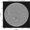 |
Fig. 1 MDI magnetogram (14 June 2002) showing the active region 09997 at 9N59E. |
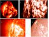 |
Fig. 2 Images of the filament. a) TRACE, 17.1 nm, 14 June 2002 18:15 UT. b) VAULT, 121.6 nm, 14 June 2002 18:15 UT. c) EIT, 30.4 nm, 14 June 2002 18:04 UT. d) BBSO, 656.3 nm, 14 June 2002 18:15 UT. The TRACE and VAULT fields of view (FOV) are 500 arcsec (diameter) and 350 × 235 arcsec, respectively. The VAULT FOV was superimposed on the EIT c) and BBSO d) images. |
2. Observations of the filament with VAULT and other instruments
The filament under study lays just north of the solar equator from 12 June 2002 to 17 June 2002. The filament separates the polarities of active region NOAA number 9997 located at 9N59E, as can be seen in the MDI magnetogram of 14 June 2002 (Fig. 1).
The filament as observed from the Big Bear Solar Observatory (BBSO) is approximately 10 arcsec wide and more than 120 arcsec long (Fig. 2d).
The Very high Angular resolution ULtraviolet Telescope (VAULT, see Korendyke et al. 2001) observed the filament during its second flight on 14 June 2002. The instrument obtained 21 images with a one-second exposure time during the flight. The spatial resolution of those images is 0.4 arcsec, which was the best ever obtained from space at the time. These observations were the first to show the detailed filament structure in H-Lyα (Fig. 2b) with high contrast; the fine structure of a filament in H-Lyα was unknown until now probably because of the lower contrast in the TRC images in 1980 (Bonnet et al. 1980).
The filament has been observed by several space and ground-based observatories as part of a coordinated campaign in support of the VAULT launch. The BBSO acquired Hα images of the filament close in time to the VAULT observations (see Fig. 2d). EIT (extreme UV imaging telescope) on board SOHO and TRACE were observing at the same time (Figs. 2c and a, respectively). Observations with the coronal diagnostic spectrometer (CDS) on board SOHO were also made as part of a joint observation programme (JOP148) with VAULT (Vourlidas et al. 2010).
To obtain a better understanding of the geometry of the filament, we searched for images of the filament when it appeared a few days earlier as a prominence (Fig. 3). The BBSO Hα image of June 11 (Fig. 3a) shows a very low-lying and compact structure. The EIT (17.1 nm and 30.4 nm) images essentially show the hot loops around the filament (at the limb) without a clear trace of absorbing material. Some morphological information came from the BBSO Hα (Fig. 3d) image, which clearly shows that the filament is rather vertical. Because of the inclination of the filament and its distance to the central meridian, it is seen edge-on; thus one only sees one flank of it (the upper and more diffuse part), and not the other one, because this is hidden behind the top of the structure corresponding to the sharp lower observed edge.
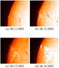 |
Fig. 3 Hα filament images from BBSO from 11 to 14 June 2002. |
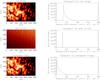 |
Fig. 4 Suppression of the dark current in VAULT images. Top: raw image and its histogram. Middle: dark current image and its histogram. Bottom: processed image and its histogram. The pixel is worth approximately 0.125 arcsec. |
3. Data processing
Of the 21 images recorded by VAULT, 17 have the same pointing and were used for the study of the filament. The first step in the data processing was to subtract the dark current from the images. The dark current was obtained by recording an image before opening the door of the instrument. The dark current image and its histogram are shown in Fig. 4, as well as an image and its histogram before and after the subtraction of the dark current. Interference from a faulty ground during science operations created a noise pattern visible in the dark current image (Vourlidas et al. 2010). Because the pattern varies from image to image, it cannot be completely subtracted out. The remaining signal fluctuates between 63 to 103 DN s-1 (22.6 to 35.9 W m-2 sr-1), which is about a factor of 40 less than the signal in the dark areas within the filament. Therefore, a simple dark-current subtraction suffices for our purposes. Besides, the aperiodic variability of the remaining dark signal does not affect our fast Fourier transform (FFT) measurements later on.
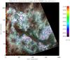 |
Fig. 5 VAULT image where the intensity contours of the coaligned BBSO image are superimposed. |
3.1. Coalignment
Because relevant pointing information is not available, VAULT and BBSO images were first visually coaligned. We then used cross-correlation to determine by successive tries the best relative angle, pixel step and relative position. When using larger steps between our guess parameters, we first decreased the resolution of those images. We then progressively returned to the initial resolution for VAULT, and made the BBSO observations to match those of VAULT, at the same time that we diminished the step of our three parameters. We empirically find that the precision of our coalignment is about 0.1 arcsec for the relative position, 10-4 radian for the relative angle, and 10-4 arcsec for the pixel pitch. The result can be seen in Fig. 5, where BBSO contours are superimposed on the VAULT image.
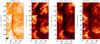 |
Fig. 6 Coaligned images of the same filament observed from left to right by: BBSO (Hα line 656.3 nm), VAULT (H-Lyα line 121.6 nm), EIT (He II line 30.4 nm), TRACE (Fe XI line 17.1 nm). Note that the Y axis of the image has been aligned along the filament. The units for X and Y axes are arcseconds. |
4. Data analysis
4.1. Fine structure of the filament
A close inspection of Fig. 2b shows the filament spine and two barbs located at its eastern part. The spine itself is made of elongated fibrils reminiscent of the SST threads. Since VAULT observes a line hotter than Hα, it is worthwhile to compare the perpendicular size of these threads. To study the fine structure of the filament, we selected the five regions of interest shown in Fig. 7. We chose areas where the emission concerns the spine itself, i.e. without “contamination” from the barbs.
At each position, we selected ten consecutive cuts separated by one pixel (see Sect. 4.3.1). To avoid any spatial smoothing, which would erase small-scale structures, we worked on each individual cut and looked at structuring in the directions perpendicular to the filament, both visually and with Fourier analysis. The results of the FFT analysis are shown and discussed in Appendix A. Indeed, in regions where threads can be isolated (especially at the borders) for some individual cuts, one can measure elemental structures down to 0.4 arcsec wide (see Fig. A.1a of Appendix A), especially in the area of cut 5. But when averaging on the ten cuts of each of the five areas, this 0.4 structuring disappears and one is left with FFT peaks at 1 to 2 arcsec (Fig. A.1b). For comparison, we also display the power spectrum of a quiet Sun cut (right-hand side of the VAULT image), which shows a peak at 30−35 arcsec (the expected supergranulation scale) (Fig. A.2a) and no significant peak at small scales (Fig. A.2b). These results confirm that in the core of the filament, these small scales cannot be detected because of the combined effects of line-of-sight and absorption, at least in broad-band images.
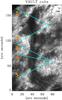 |
Fig. 7 Location of cuts across the filament selected for the search of spatial characteristics. |
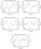 |
Fig. 8 Cuts across the filament as defined in Fig. 7. H-Lyα (VAULT) is in magenta and Hα (BBSO) is in blue. Error bars represent photon noise. |
4.2. Filament contrast
Another important result concerns the contrast between the filament and the near-by active and quiet Sun. Using the mean cut of Fig. 9 and a (measured) ratio between the active and quiet Sun H-Lyα intensities, we can derive that the LRI is about 0.2. Here we define the LRI as the ratio  , where IF is the lowest intensity in the filament, and IN is an average intensity around the filament, which is assumed to represent the intensity of the line incident on the (invisible) lower part of the filament (for a discussion, see the cloud model, e.g. by Mein et al. 1996). We can now use this value for deriving some (average) properties of the filament through a comparison with the models and the predicted LRIs of Table I of Gouttebroze et al. (1986). Of course, we only used the data concerning the horizontal (“H”) and cylindrical configurations. One can see that high temperature and very high density loop models must be discarded. The 0.2 value for the LRI is consistent with a wide range of temperatures and pressures. It should be pointed out that this result, which is shown to be valid for cylindrical geometries (Gouttebroze et al. 1986), depends on the adopted thickness of the layer and only indicates that to obtain this value of the LRI, the pressure should be neither too high (the radiation is then dominated by thermal emission) nor too low (the opacity is then too low) (see Fig. 12 of Gouttebroze et al. 1986). Another important related question concerns the origin of the H-Lyα photons as recorded by the wide bandpass of VAULT. We defer this question to the discussion section.
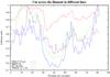 |
Fig. 9 Cut at position 3 of the filament in different lines: VAULT H-Lyα is plotted in BLUE, BBSO Hα in red, EIT 30.4 nm in green, and TRACE 17.1 nm in PURPLE. The arbitrary units are obtained by dividing the cut intensity by its maximum value. |
4.3. Multiwavelength analysis
At the time of the VAULT flight (14 June 2002 at 18:15 UT), ground-based and space observations were performed in the frame of a support campaign (Fig. 2). To analyse the environment of the observed filament, we selected a small region containing the filament and superimposed the images taken in H-Lyα (VAULT), Hα (BBSO), He II 30.4 nm (EIT), and Fe IX/X 17.1 nm (TRACE). The procedure relied on image correlation (facilitated by the filament being dark in all lines). We also oriented the filament’s spine vertically in the four images to ease the comparison. The resulting images are shown in Fig. 6.
4.3.1. The search for filament extensions
Since filaments are usually “defined” in the Hα line, we first focused on the H-Lyα behaviour compared to Hα to detect possible filament extensions in the optically thick H-Lyα line. We used cuts perpendicular to the filament spine at selected locations shown on the H-Lyα image of Fig. 7. Our main selection criterion was to avoid barbs where the filament extensions might be confused. Moreover, at each position, we averaged ten consecutive cuts separated by 1 pixel. The resulting cuts are displayed in Fig. 8. The error bars correspond to the statistical noise. In all cuts, the H-Lyα absorbing feature is wider than that in Hα. In some cases (cuts 3 and 4), it is about twice as large. In cuts 1−3, and 5, the H-Lyα cuts are sharper on the left-hand side than on the right-hand side. We return to this result in the discussion. We also compared H-Lyα and Hα cuts at position 3 with cuts in the He II and Fe IX/X lines (Fig. 9). This position, free of any barb, is in our view representative of the structure of the filament across its spine, especially as far as extensions are concerned. All cuts were normalised to the maximum values in the respective lines. It is not surprising to have similar behaviours of H-Lyα and He II since these two resonance lines are optically thick, but because the He II line is less optically thick, the width of the filament is slightly narrower than the H-Lyα width. In contrast, it is a priori surprising that the Fe IX/X width is comparable to the H-Lyα width. This absorption takes place in the H, He I and He II Lyman continua, which are less thick than the H and He II resonance lines. We envisage two possibilities: either the absorbing material also exists at temperatures higher than 20 000 K, and consequently the absorption by He and H+ is enhanced, or we also deal with lack of emission (“emissivity blocking”) in the coronal line.
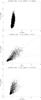 |
Fig. 10 Scatter plots of H-Lyα with regard to Hα (top), He II (middle) and Fe IX/X (bottom). The plotted intensities are taken from the images shown in Fig. 6. For each image, intensities were divided by the mean intensity in the image. |
4.3.2. EUV, Hα and H-Lyα correlations
In Fig. 10 we present the scatter plots of the H-Lyα intensity with regard to the Hα, He II, and Fe XI intensities. The data considered for the plots are from the coaligned images (Fig. 6). For each wavelength, intensities were divided by the mean intensity. One can distinguish the group of points corresponding to the filament (lower parts). Some saturation of the H-Lyα intensity versus Hα intensity occurs towards low intensities, which is due to strong but finite opacity (see Fig. 10 top). The range of Hα values at very low H-Lyα intensities can be understood in various ways: because the Hα filament is less extended than the H-Lyα filament, and also because the H-Lyα line is very optically thick, combined with a lower Hα optical thickness, a “saturation” of the line (towards low intensities) is possible for the H-Lyα line, but not the Hα line. Note also the much stronger contrast in H-Lyα over the whole field-of-view compared to Hα (it is six times higher in H-Lyα). This certainly reflects the different nature of the lines: H-Lyα is an emission line, Hα an absorption line.
We tried to compare our results with the H-Lyα vs. Hα correlations obtained from TRC, Sacramento Peak and MSDP observations by Wiik et al. (1996). These authors separate plage and quiet Sun from filament and quiet Sun and plot their values as normalised to average (probably) uncalibrated values. Consequently, the comparison is difficult. However, the very large contrast in H-Lyα is clearly visible. As for the correlation between H-Lyα (121.6 nm) and He II (30.4 nm) (Fig. 10 middle), it also shows the presence of the filament at very low H-Lyα and He II intensities. Some linear correlation is apparent, which we interpret as evidence that not only H-Lyα but also He II is very optically thick in the filament and saturates towards close-to-zero intensities. In Fig. 10 (middle), one can distinguish two regimes: a linear correlation for very low intensities which correspond to the filament values, and another linear correlation, with a steeper slope and higher dispersion for all other intensities. This linear correlation fits the correlation between full disk measurements in H-Lyα and He II well (Auchère 2005). A comparison with the recent He modelling of Gouttebroze & Labrosse (2009) is made difficult because these authors work with a vertical cylinder of which they compute the exiting horizontal radiation. However, one can say that the significant absorption in He II (Fig. 9) comes from absorbing material at about 20 000 K (see Fig. 1 of Gouttebroze & Labrosse 2009).
A reduced contrast (about 3) also exists in the 17.1 nm band (Fig. 10 bottom), and the explanation is similar to that for Hα, since the coronal lines present in the 17.1 nm band are affected by the continuum absorption of He I and He II in the filament. A combination of observations (at 19.5 nm) and modelling (Heinzel et al. 2008) has shown that the opacity in the 19.5 nm band and consequently in the 17.1 nm band is close to the opacity of Hα. From the three parts of Fig. 10, we see that the range of variation of the H-Lyα intensity is far wider than the ranges of He II and Fe IX, especially towards the lower values that correspond to the filament and its environment.
On the basis of Figs. 9 and 10, we conclude that the H-Lyα line is a very efficient tracer of cool material within and outside of the filament.
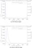 |
Fig. 11 Integrated contribution function (in blue) and temperature (in magenta) as a function of the filament depth. |
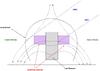 |
Fig. 12 Filament and its environment in a plane perpendicular to the horizontal photosphere and to the main axis of the filament. The dot-dashed lines tentatively trace the magnetic field. Depending on the line of sight, the absorbing material next to the filament is visible (LOS2) or can be hidden (LOS1); in this case the edge of the filament appears to be sharp. See also Fig. 4 of Schwartz et al. (2004). |
5. Discussion
We have presented the joint analysis of images of an active region filament taken in the H-Lyα, Hα, He II and Fe IX/X lines obtained with VAULT, BBSO, EIT, and TRACE instrumentation, with some focus on the combined H-Lyα and Hα observations. The unique spatial resolution of VAULT allowed us to confirm the fine structuring of filaments down to a scale of 1 to 2 arcsec (and for some cuts at 0.4 arcsec, close to the limit of the spatial resolution). The differences with the SST observations of a quiescent filament are quite clear: in the H-Lyα line and in contrast to high-resolution Hα observations of barbs, there is no evidence of fine structure crossing the filament. But we also observe elongated fibrils along the filament itself. It is difficult to assess whether this difference is due to the different nature of the filaments (active region vs. quiescent) or the peculiarities of the two lines. About the second hypothesis, it is quite certain that the moderately optically thick Hα line traces the coolest and deepest (inside the filament) material. On the contrary, the optically thick H-Lyα line (thicker by about five orders of magnitude) traces the cool and warm external material. Using a model introduced by P. Schwartz (Schwartz et al. 2012), we computed the integrated contribution function (Fig. 11) to find out that the H-Lyα emission is essentially coming from 20 000 K material, which is consequently situated in the external transition region. Therefore, we can propose the following picture for the fine threads: they certainly have individual and well-separated cool cores, but a portion of them shares a common transition region to the corona. This results in a smoothing of the H-Lyα intensity in the direction perpendicular to the fibrils. This smoothing does not erase the presence of fine structure down to less than 1 to 2 arcsec (about 0.4 arcsec), however, as shown by a FFT analysis. This smoothing also contributes to a (small) extension of the absorption across the filament. This result is also valid for the He II line, which is formed at a temperature higher than H-Lyα.
Let us now address the question of (quiescent) filament extensions that were noticed through strong absorption of EUV lines below the Lyman continuum (Heinzel et al. 2003; Schwartz et al. 2004; Anzer et al. 2007; Heinzel et al. 2008). Figure 9 clearly shows that on the left-hand side of the filament (lower latitude), there is no signature of absorption in the H or the He II Lyman α lines, although the H-Lyα line is about five orders of magnitude thicker than the Lyman continuum. The Fe IX/X emission is also depleted. On the right-hand side of the filament (higher latitude) (Fig. 9), we notice a deep absorption in H and He II resonance lines, and some depletion in the Fe line (but not in Hα).
On the left-hand side of the filament, the Fe IX/X results may be understood if we follow the conclusion of Heinzel et al. (2001), who strongly support the idea of a coronal void around quiescent filaments, which explains why the H and He II emissions are unchanged with respect to Hα, and the Fe IX/X is depleted. However, the right-hand side clearly shows absorption. In this respect, it is difficult to understand why there would be such an asymmetry in the morphology of the filament environment.
To (tentatively) explain both observations, we return to the observation geometry and realize that the filament is at a low northern latitude, high eastern longitude and is inclined (in projection) about 30° from the equator. In the bottom (lower latitude) part, below the observed filament, some cool material is certainly present. But the lower border (in latitude and longitude) of the filament corresponds to the top of the filament whose projection lies at lower latitude and higher longitude than the actual ones. Consequently, the bottom material is invisible. The upper border (in latitude and longitude) of the filament, however, corresponds to the (hot) extension of the filament. If so, absorbing (cool) material could be present on both sides of the filament. This picture with two components, a coronal void and absorbing material on both sides, is summarized in Fig. 12 where LOS1 aims at the southern edge of the filament, while LOS 2 aims at its northern edge. The cartoon localizes the filament in a coronal void (Tandberg-Hanssen 1995) and flanks it with absorbing material, only visible on the right-hand side, and masked on the left-hand side. Of course, we would like to have some information about the extension (altitude and thickness) of this absorbing material (see Schwartz et al. 2004). The only information we are certain of is that its altitude is lower than the height of the filament. The absence of information on the geometrical thickness does not allow a density estimation. Whether this picture is specific to active region filaments only remains to be proved through additional measurements on quiescent and active filaments.
6. Conclusion
The value of the multiwavelength analysis of a filament with imaging observations with the highest spatial resolution was ascertained. The structuring of the plasma in elongated threads at 0.4 and 1 to 2 arcsec level was established in the H-Lyα line. The presence of absorbing plasma and possibly coronal void around the filament was derived. Continuous observations in the H-Lyα line over a few days would have allowed us to derive the geometry of the filament and the adjacent absorbing regions, and consequently their density properties.
Simultaneous spectroscopic observations would be invaluable, especially in the optically thick H-Lyα and H-Lyβ lines, because different points in the line profile allow one to scan the observed structure in depth (Vial et al. 2007).
Online material
Appendix A: Analysis of the fine structure of the H-Lyα filament through FFT of perpendicular cuts
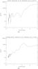 |
Fig. A.1 Square of the modulus of the FFT as a function of spatial frequency (converted in spatial scale) limited to the high spatial frequencies for cuts in the filament. a) Subcut 5 of cut area 5. b) Average of cuts of the area 1. |
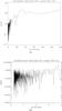 |
Fig. A.2 Square of the modulus of the FFT as a function of spatial frequency (converted in spatial scale) for a cut in the quiet Sun at X = 3000 of Fig. 4. a) Full power spectrum obtained for the cut. b) Zoom on the high frequencies. |
As mentioned in Sects. 4.1 and 4.3.1, we analysed ten consecutive cuts made at the five positions shown in Fig. 7. We used the usual method of subtracting the average values and of tapering at both ends to avoid unwanted high frequencies. We show in Figs. A.1a and b the square of the modulus of the FFT as a function of spatial frequency (converted in spatial scale) limited to the high- frequency region. Figure A.1a is an example of an individual cut (in region 5) showing power at the 0.4 arcsec scale. We performed a power spectrum estimation through reducing the spectral analysis bandwidth. Between 0.24 and 2 arcsec, our peak at 0.38 arcsec is above 2.5 times the standard deviation, providing a confidence level higher than 95%. We also show an average power spectrum of area 1 (Fig. A.1b) where it is difficult to find power at 0.4 arcsec but where the 2 arcsec scale can definitely be identified. (Other cuts show some power around 1 arcsec.) Finally, for the sake of comparison, we show in Fig. A.2 the FFT square power of a vertical cut in the quiet Sun image performed at X = 3000 (Fig. 4). Figure A.2a displays the full power spectrum where one can distinguish power at about 30 − 35 arcsec, typical of the supergranulation. The zoom performed into the high-frequency region (Fig. A.2b) does not show any power below 4 arcsec.
Acknowledgments
Jean-Claude Vial acknowledges the ISSI support in the frame of the “Spectroscopy and Imaging of Quiescent and Eruptive Prominences from Space” working team, headed by N. Labrosse, and is grateful to V. Abramenko, who helped us with special BBSO files, to L. Golub, for the TRACE image, and to P. Schwartz, who provided the filament model. The authors thank the anonymous referee, who helped them to improve the paper. The work of A. Vourlidas was supported by various NASA grants to the Naval Research Laboratory.
References
- Anzer, U., Heinzel, P., & Fárnik, F. 2007, Sol. Phys., 242, 43 [NASA ADS] [CrossRef] [Google Scholar]
- Auchère, F. 2005, ApJ, 622, 737 [NASA ADS] [CrossRef] [Google Scholar]
- Bonnet, R. M., Decaudin, M., Bruner, Jr., E. C., Acton, L. W., & Brown, W. A. 1980, ApJ, 237, L47 [NASA ADS] [CrossRef] [Google Scholar]
- Dunn, R. B. 1959, ApJ, 130, 972 [NASA ADS] [CrossRef] [Google Scholar]
- Engvold, O., Jakobsson, H., Tandberg-Hanssen, E., Gurman, J. B., & Moses, D. 2001, Sol. Phys., 202, 293 [NASA ADS] [CrossRef] [Google Scholar]
- Gouttebroze, P., & Labrosse, N. 2009, A&A, 503, 663 [NASA ADS] [CrossRef] [EDP Sciences] [Google Scholar]
- Gouttebroze, P., Vial, J. C., & Tsiropoula, G. 1986, A&A, 154, 154 [NASA ADS] [Google Scholar]
- Gunár, S., Heinzel, P., Schmieder, B., Schwartz, P., & Anzer, U. 2007, A&A, 472, 929 [NASA ADS] [CrossRef] [EDP Sciences] [Google Scholar]
- Heinzel, P. 2007, in The Physics of Chromospheric Plasmas, ed. P. Heinzel, I. Dorotovič, & R. J. Rutten, ASP Conf. Ser., 368, 271 [Google Scholar]
- Heinzel, P., & Anzer, U. 2003, in Stellar Atmosphere Modeling, ed. I. Hubeny, D. Mihalas, & K. Werner, ASP Conf. Ser., 288, 441 [Google Scholar]
- Heinzel, P., & Anzer, U. 2006, ApJ, 643, L65 [NASA ADS] [CrossRef] [Google Scholar]
- Heinzel, P., Schmieder, B., & Tziotziou, K. 2001, ApJ, 561, L223 [NASA ADS] [CrossRef] [Google Scholar]
- Heinzel, P., Anzer, U., & Schmieder, B. 2003, Sol. Phys., 216, 159 [NASA ADS] [CrossRef] [Google Scholar]
- Heinzel, P., Schmieder, B., Fárník, F., et al. 2008, ApJ, 686, 1383 [NASA ADS] [CrossRef] [Google Scholar]
- Korendyke, C. M., Vourlidas, A., Cook, J. W., et al. 2001, Sol. Phys., 200, 63 [NASA ADS] [CrossRef] [Google Scholar]
- Labrosse, N., Heinzel, P., Vial, J.-C., et al. 2010, Space Sci. Rev., 151, 243 [Google Scholar]
- Lin, Y., Engvold, O., Rouppe van der Voort, L., Wiik, J. E., & Berger, T. E. 2005, Sol. Phys., 226, 239 [NASA ADS] [CrossRef] [Google Scholar]
- Lin, Y., Engvold, O., Rouppe van der Voort, L. H. M., & van Noort, M. 2007, Sol. Phys., 246, 65 [NASA ADS] [CrossRef] [Google Scholar]
- Mackay, D. H., Karpen, J. T., Ballester, J. L., Schmieder, B., & Aulanier, G. 2010, Space Sci. Rev., 151, 333 [NASA ADS] [CrossRef] [Google Scholar]
- Mein, N., Mein, P., Heinzel, P., et al. 1996, A&A, 309, 275 [NASA ADS] [Google Scholar]
- Patsourakos, S., & Vial, J.-C. 2002, Sol. Phys., 208, 253 [NASA ADS] [CrossRef] [Google Scholar]
- Patsourakos, S., Gouttebroze, P., & Vourlidas, A. 2007, ApJ, 664, 1214 [NASA ADS] [CrossRef] [Google Scholar]
- Scharmer, G. B., Kiselman, D., Löfdahl, M. G., & Rouppe van der Voort, L. H. M. 2003, ASP Conf. Ser. 307, ed. J. Trujillo-Bueno, & J. Sanchez Almeida, 3 [Google Scholar]
- Schmieder, B., Lin, Y., Heinzel, P., & Schwartz, P. 2004, Sol. Phys., 221, 297 [NASA ADS] [CrossRef] [Google Scholar]
- Schwartz, P., Heinzel, P., Anzer, U., & Schmieder, B. 2004, A&A, 421, 323 [NASA ADS] [CrossRef] [EDP Sciences] [Google Scholar]
- Schwartz, P., Heinzel, P., Schmieder, B., & Anzer, U. 2006, A&A, 459, 651 [NASA ADS] [CrossRef] [EDP Sciences] [Google Scholar]
- Schwartz, P., Schmieder, B., Heinzel, P., & Kotrc, P. 2012, Sol. Phys., submitted [Google Scholar]
- Tandberg-Hanssen, E. 1995, The nature of solar prominences, Astrophys. Space Sci. Libr., 199 [Google Scholar]
- Tsiropoula, G., Alissandrakis, C., Bonnet, R. M., & Gouttebroze, P. 1986, A&A, 167, 351 [NASA ADS] [Google Scholar]
- Vial, J. C. 1982, ApJ, 253, 330 [NASA ADS] [CrossRef] [Google Scholar]
- Vial, J.-C. 2006a, in Proceedings of the Third French-Chinese Solar meeting, Shanghai 2005, ed. C. Fang, B. Schmieder, & M. D. Ding (Nanjing University Press), 184 [Google Scholar]
- Vial, J.-C. 2006b, in SOHO-17, 10 Years of SOHO and Beyond, ESA SP, 617 [Google Scholar]
- Vial, J.-C., Boutry, C., & Wilhelm, K. 2005, in The Dynamic Sun: Challenges for Theory and Observations, ESA SP, 600 [Google Scholar]
- Vial, J.-C., Ebadi, H., & Ajabshirizadeh, A. 2007, Sol. Phys., 246, 327 [NASA ADS] [CrossRef] [Google Scholar]
- Vourlidas, A., Klimchuk, J. A., Korendyke, C. M., Tarbell, T. D., & Handy, B. N. 2001, ApJ, 563, 374 [NASA ADS] [CrossRef] [Google Scholar]
- Vourlidas, A., Sanchez Andrade-Nuño, B., Landi, E., et al. 2010, Sol. Phys., 261, 53 [NASA ADS] [CrossRef] [Google Scholar]
- Wiik, J. E., Foing, B. H., Martens, P., Fleck, B., & Schmieder, B. 1996, Adv. Space Res., 17, 105 [NASA ADS] [CrossRef] [Google Scholar]
All Figures
|
Fig. 1 MDI magnetogram (14 June 2002) showing the active region 09997 at 9N59E. |
| In the text | |
|
Fig. 2 Images of the filament. a) TRACE, 17.1 nm, 14 June 2002 18:15 UT. b) VAULT, 121.6 nm, 14 June 2002 18:15 UT. c) EIT, 30.4 nm, 14 June 2002 18:04 UT. d) BBSO, 656.3 nm, 14 June 2002 18:15 UT. The TRACE and VAULT fields of view (FOV) are 500 arcsec (diameter) and 350 × 235 arcsec, respectively. The VAULT FOV was superimposed on the EIT c) and BBSO d) images. |
| In the text | |
|
Fig. 3 Hα filament images from BBSO from 11 to 14 June 2002. |
| In the text | |
|
Fig. 4 Suppression of the dark current in VAULT images. Top: raw image and its histogram. Middle: dark current image and its histogram. Bottom: processed image and its histogram. The pixel is worth approximately 0.125 arcsec. |
| In the text | |
|
Fig. 5 VAULT image where the intensity contours of the coaligned BBSO image are superimposed. |
| In the text | |
|
Fig. 6 Coaligned images of the same filament observed from left to right by: BBSO (Hα line 656.3 nm), VAULT (H-Lyα line 121.6 nm), EIT (He II line 30.4 nm), TRACE (Fe XI line 17.1 nm). Note that the Y axis of the image has been aligned along the filament. The units for X and Y axes are arcseconds. |
| In the text | |
|
Fig. 7 Location of cuts across the filament selected for the search of spatial characteristics. |
| In the text | |
|
Fig. 8 Cuts across the filament as defined in Fig. 7. H-Lyα (VAULT) is in magenta and Hα (BBSO) is in blue. Error bars represent photon noise. |
| In the text | |
|
Fig. 9 Cut at position 3 of the filament in different lines: VAULT H-Lyα is plotted in BLUE, BBSO Hα in red, EIT 30.4 nm in green, and TRACE 17.1 nm in PURPLE. The arbitrary units are obtained by dividing the cut intensity by its maximum value. |
| In the text | |
|
Fig. 10 Scatter plots of H-Lyα with regard to Hα (top), He II (middle) and Fe IX/X (bottom). The plotted intensities are taken from the images shown in Fig. 6. For each image, intensities were divided by the mean intensity in the image. |
| In the text | |
|
Fig. 11 Integrated contribution function (in blue) and temperature (in magenta) as a function of the filament depth. |
| In the text | |
|
Fig. 12 Filament and its environment in a plane perpendicular to the horizontal photosphere and to the main axis of the filament. The dot-dashed lines tentatively trace the magnetic field. Depending on the line of sight, the absorbing material next to the filament is visible (LOS2) or can be hidden (LOS1); in this case the edge of the filament appears to be sharp. See also Fig. 4 of Schwartz et al. (2004). |
| In the text | |
|
Fig. A.1 Square of the modulus of the FFT as a function of spatial frequency (converted in spatial scale) limited to the high spatial frequencies for cuts in the filament. a) Subcut 5 of cut area 5. b) Average of cuts of the area 1. |
| In the text | |
|
Fig. A.2 Square of the modulus of the FFT as a function of spatial frequency (converted in spatial scale) for a cut in the quiet Sun at X = 3000 of Fig. 4. a) Full power spectrum obtained for the cut. b) Zoom on the high frequencies. |
| In the text | |
Current usage metrics show cumulative count of Article Views (full-text article views including HTML views, PDF and ePub downloads, according to the available data) and Abstracts Views on Vision4Press platform.
Data correspond to usage on the plateform after 2015. The current usage metrics is available 48-96 hours after online publication and is updated daily on week days.
Initial download of the metrics may take a while.