| Issue |
A&A
Volume 541, May 2012
|
|
|---|---|---|
| Article Number | A35 | |
| Number of page(s) | 18 | |
| Section | Interstellar and circumstellar matter | |
| DOI | https://doi.org/10.1051/0004-6361/201117876 | |
| Published online | 24 April 2012 | |
Bridging the gap: disk formation in the Class 0 phase with ambipolar diffusion and Ohmic dissipation
1 Jülich Supercomputing Centre (JSC), Institute for Advanced Simulation (IAS), FZ Jülich, 52425 Jülich, Germany
e-mail: This email address is being protected from spambots. You need JavaScript enabled to view it.
2 Department of Physics & Astronomy, The University of Western Ontario, 1151 Richmond St., London, ON, N6A 3K7, Canada
e-mail: This email address is being protected from spambots. You need JavaScript enabled to view it.
3 Rudolf Peierls Centre for Theoretical Physics, University of Oxford, 1 Keble Road, Oxford OX1 3NP, UK
4 Einstein Postdoctoral Fellow, Department of Astrophysical Sciences, Princeton University, Peyton Hall, 4 Ivy Lane, Princeton, NJ 08544, USA
e-mail: This email address is being protected from spambots. You need JavaScript enabled to view it.
Received: 11 August 2011
Accepted: 21 February 2012
Abstract
Context. Ideal magnetohydrodynamical (MHD) simulations have revealed catastrophic magnetic braking in the protostellar phase, which prevents the formation of a centrifugal disk around a nascent protostar.
Aims. We determine if non-ideal MHD, including the effects of ambipolar diffusion and Ohmic dissipation determined from a detailed chemical network model, will allow for disk formation at the earliest stages of star formation.
Methods. We employ the axisymmetric thin-disk approximation in order to resolve a dynamic range of 9 orders of magnitude in length and 16 orders of magnitude in density, while also calculating partial ionization using up to 19 species in a detailed chemical equilibrium model. Magnetic braking is applied to the rotation using a steady-state approximation, and a barotropic relation is used to capture the thermal evolution.
Results. We resolve the formation of the first and second cores, with expansion waves at the periphery of each, a magnetic diffusion shock, and prestellar infall profiles at larger radii. Power-law profiles in each region can be understood analytically. After the formation of the second core, the centrifugal support rises rapidly and a low-mass disk of radius ≈ 10 R⊙ is formed at the earliest stage of star formation, when the second core has mass ~10-3 M⊙. The mass-to-flux ratio is ~104 times the critical value in the central region.
Conclusions. A small centrifugal disk can form in the earliest stage of star formation, due to a shut-off of magnetic braking caused by magnetic field dissipation in the first core region. There is enough angular momentum loss to allow the second collapse to occur directly, and a low-mass stellar core to form with a surrounding disk. The disk mass and size will depend upon how the angular momentum transport mechanisms within the disk can keep up with mass infall onto the disk. Accounting only for direct infall, we estimate that the disk will remain ≲10 AU, undetectable even by ALMA, for ≈ 4 × 10⁴ yr, representing the early Class 0 phase.
Key words: magnetohydrodynamics (MHD) / accretion, accretion disks / stars: formation / protoplanetary disks / stars: magnetic field
© ESO, 2012
1. Introduction
Near the beginning of the star formation process, prestellar cores are observed to be rotating (e.g., Goldsmith & Arquilla 1985; Goodman et al. 1993; Caselli et al. 2002). At the end of the process, observations show nearly all Class II objects to be surrounded by rotating disks of size ≳ 100 AU, likely in centrifugal balance undergoing Keplerian rotation (see, e.g., Andrews & Williams 2005; Williams & Cieza 2011, and references therein). Observational data concerning what happens in between those two snapshots is relatively scarce. Currently, there is no evidence for the presence of centrifugal disks larger than ≈50 AU around Class 0 or Class I objects (e.g., Maury et al. 2010). However, there are outflows observed around these young objects, commonly linked to disk accretion. Disks must therefore form with a small size and grow over time. The dearth of observational data at smaller scales will be remedied by ALMA. In the meantime, the evolution of angular momentum and the formation of a centrifugal disk have to be studied theoretically and numerically.
In order to form stars of the observed sizes and rotation rates, most of the angular momentum has to be removed from the infalling gas. This is the classical angular momentum problem (e.g., Spitzer 1978). The required reduction of angular momentum is often credited to magnetic braking, which acts during the contraction and collapse by linking the core with its envelope and transferring angular momentum (see Basu & Mouschovias 1994, and references therein). Recent numerical simulations of protostellar collapse under the assumption of ideal magnetohydrodynamics (MHD) have suggested the converse problem, namely that cores may experience catastrophic magnetic braking. This is the result that an extremely pinched magnetic field configuration has enough strength and exerts a long enough lever arm on the inner regions of collapse that magnetic braking can suppress the formation of a centrifugal disk entirely.
Catastrophic magnetic braking was first demonstrated by Allen et al. (2003), who used two-dimensional (2D) axisymmetric calculations. Subsequent ideal MHD simulations by Mellon & Li (2008) in 2D and Hennebelle & Fromang (2008) in three dimensions (3D) showed that catastrophic magnetic braking occurs for initially aligned (magnetic field parallel to rotation axis) rotators in which the magnetic field is strong enough that μ ≲ 10, where μ is the initial core mass-to-flux ratio normalized to its critical value for gravitational collapse. Disk formation in ideal MHD then requires at least μ ≳ 10, which is significantly greater than the typical value ~2 for dense cores determined from observations (e.g., Troland & Crutcher 2008). Furthermore, Mellon & Li (2009) found that the inclusion of non-ideal effects of Ohmic dissipation and ambipolar diffusion in a 2D model was not sufficient to enable disk formation on scales of ≳ 10 AU from the center that were resolvable in their simulation. In a newer 2D model that also includes the Hall term of non-ideal MHD, Li et al. (2011) again find essentially the same result. All of the above simulations have an inner resolution limit of ≈ 10 AU due to the use of a sink cell or an artificially stiff equation of state at high densities. Since these simulations also terminated soon after the central stellar core formed, the main common result of these simulations is that large ~100 AU disks (as observed around Class II objects) cannot form during the early Class 0 phase. A 3D ideal MHD model by Hennebelle & Ciardi (2009) that starts with a non-aligned rotator, also finds catastrophic magnetic braking on these scales but within a smaller range of μ ≲ 3. The effect of numerical reconnection may account for some of the differences amongst these models. All of the above works leave open the possibility that a small disk may actually form within the inner ~10 AU during the earliest phases of star formation.
An interesting question is: can a very small disk form in the innermost regions (near the protostar) in the case of ideal MHD? Galli et al. (2006) developed a simplified analytic model with a split-monopole magnetic field to show that catastrophic magnetic braking extends to the stellar surface in the flux-frozen limit. Krasnopolsky & Königl (2002) and Braiding & Wardle (2012) employed self-similar non-ideal MHD models in the thin-disk approximation, using the prescription for steady-state magnetic braking developed by Basu & Mouschovias (1994). Depending on different levels of effective diffusivity, they found either catastrophically-braked or disk-formation solutions. However, the diffusivity was parametrized in a way that preserved self-similarity, and its magnitude and functional form did not make contact with microphysical models. Consequently, a prediction for whether or not disks may actually form was not possible.
Our work fills the gap of numerically studying disk formation in the early Class 0 phase down to scales smaller than a stellar radius. In a previous paper (Dapp & Basu 2010, hereafter DB10) we followed the evolution of a collapsing molecular cloud core in axisymmetric thin-disk geometry all the way to protostellar densities (n > 1020 cm-3). We found that Ohmic dissipation alone (in a simplified form) reduces the magnetic field strength sufficiently to render magnetic braking within the first core ineffective. As a result, a centrifugal disk can indeed form around the second core (the protostar).
The only other related MHD models that resolve the stellar core are the 3D non-ideal MHD simulations by Machida et al. (2006, 2007) and Machida & Matsumoto (2011), who also used a simplified treatment of Ohmic dissipation. In most of their published models, the evolution was halted at up to ten days after the second core was formed, due to time-step restrictions, and the formation of a centrifugal disk was not studied. Very recent work (Machida & Matsumoto 2011) follows disk formation in one MHD model, and its relation to our work is discussed in Sect. 8.
In this paper, we increase realism by employing a detailed chemical network including the effect of grains to calculate partial ionization and the resulting Ohmic and ambipolar diffusivities. We use the method presented in Kunz & Mouschovias (2009). Both Ohmic dissipation and ambipolar diffusion gain importance with the formation of the first core (e.g., Li & McKee 1996; Contopoulos et al. 1998; Desch & Mouschovias 2001). We follow the evolution of the core to stellar sizes, using a multi-fluid approach that includes important inelastic collisions between gas-phase species and grains. We also study the effect of different grain sizes. We model four gas-phase species and up to five different grain sizes with three charge states (singly positively- or negatively charged, and neutral) for each grain size. We demonstrate that Ohmic dissipation and ambipolar diffusion can reduce the efficiency of magnetic braking in the inner regions enough to allow for the formation of a centrifugally-supported disk. There is dramatic magnetic flux loss, and a small disk can form in a very early phase of evolution. We propose a disk formation scenario in which the disk remains ≲ 10 AU during the Class 0 phase, and subsequently expands significantly due to internal angular momentum transport mechanisms such as magnetorotational instability (MRI) or gravitational torques (e.g., Balbus & Hawley 1991; Vorobyov & Basu 2007).
This paper is structured the following way. In Sect. 2 we formulate the problem and describe the method of solution. Section 3 discusses the implementation of magnetic braking, while Sect. 4 outlines the derivation of the induction equation. Section 5 details the chemical model used to calculate the abundances of each species and Sect. 6 contains the description of our initial conditions. Readers mainly interested in our results may proceed directly to Sect. 7. The discussion is found in Sect. 8, and we summarize our findings in Sect. 9.
2. Method
We solve the equations of non-ideal MHD for a rotating, axisymmetric thin disk made up of partially-ionized gas (Basu & Mouschovias 1994). In the thin-disk approximation, all quantities are assumed to be uniform over one scale height of the disk. It is applicable as long as the half-thickness of the disk remains small compared to the radius of the disk. Fiedler & Mouschovias (1993) showed that an initially cylindrical cloud quickly flattens parallel to the magnetic field before any significant collapse in the radial direction occurs, and a oblate cloud is formed that can be described by the thin-disk approximation (see also Basu & Mouschovias 1994). While this approximation breaks down at the interfaces of the first core and in the second core, it holds well in most of the cloud. It allows us to follow the evolution to very high densities and very small scales with realistic physics (non-ideal MHD and sophisticated chemical model), and does not require a lot of computation time.
We solve the following system of equations, derived by integrating the MHD equations over the z-direction and assuming axisymmetry: 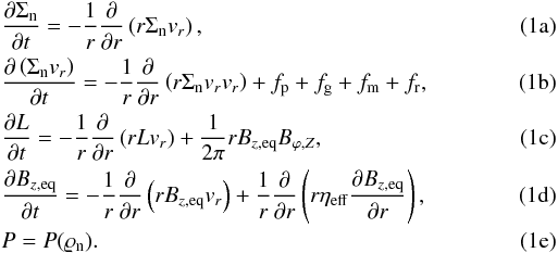 Here, Σn is the mass column density of the neutrals, vr is the radial velocity, and L ≡ ΣnΩr2 is the angular momentum per unit area. The mass volume density is denoted by ϱn. The forces fp, fg, fm, and fr, as well as the magnetic field components (Bz,eq, Br,Z, and Bϕ,Z) are discussed below (see Eqs. (6) as well as (7a) and (7b)). We do not include a separate continuity equation for the grains since no significant change of the dust-to-gas ratio occurs beyond a number density of n ≈ 106 cm-3 (Ciolek & Mouschovias 1996; Kunz & Mouschovias 2010). Due to the very low ionization fraction in the modeled core, we neglect the inertia of all species but the neutral molecular gas.
We include the effect of both ambipolar diffusion (e.g., Mestel & Spitzer 1956; Mouschovias 1979) and Ohmic dissipation (e.g., Nakano et al. 2002) in an effective resistivity ηeff, which we derive from microphysical considerations in Sect. 4. Note that we do not assume the resistivity to be spatially constant by pulling it outside all spatial derivatives, which is different from Machida et al. (2007). We ignore the contribution of the third non-ideal MHD effect – the Hall effect (e.g., Wardle 2007) – in this paper, and leave that for future work.
For computational ease, we use the barotropic relation Eq. (1e) instead of a detailed energy equation. Following DB10, we parametrize the temperature-density relation of Masunaga & Inutsuka (2000) in the following way: 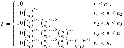 (2)In this expression, the temperature T is given in units of K. The number densities1n at which the power laws in the temperature–density relation change are n1 = 3 × 1010 cm-3, n2 = 1013 cm-3, n3 = 3 × 1016 cm-3, and n4 = 1021 cm-3.
We transform this temperature–density relation into a pressure–density relation using the ideal gas law  (3)Here, P is the thermal pressure and kB is Boltzmann’s constant. We calculate the thermal midplane pressure of the neutrals in our thin disk self-consistently, including the effects of the weight of the gas column, external pressure, magnetic pressure, and the effect of a central star (once present, with mass M★):
 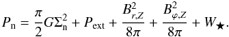 (4)Here, W★ is the extra vertical squeezing due to the star’s gravity integrated over the disk’s finite thickness. The external pressure is fixed at
  , where G is the gravitational constant and Σ0 is the initial central neutral column density. We set W★ = 0, and interpolate ϱn from the pressure-density relation found earlier. If a central object is present (after the formation of the second core, and after introduction of the sink cell), we then insert the so-determined approximation to ϱn and the disk’s half-thickness Z = Σn/2ϱn into
 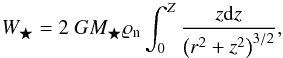 (5)where z is the vertical coordinate, and iterate this procedure until ϱn converges. The result also allows us to find the midplane temperature of our disk using Eq. (3). It is very similar to that found in an axisymmetric
  simulation with explicit radiative transfer added (Kunz & Mouschovias 2010). Note that the extra squeezing from the protostar also flattens the disk further, helping to justify the thin-disk approximation.
Once the second core forms, at a central number density of ≈ 1020 cm-3, we introduce a sink cell of size ≈ 3 R⊙ (which is only slightly larger than the second core). We remap the computational domain to a new grid with the sink as the innermost cell. The first neighboring cell outside the sink has an extent of only ≈ 10-3 AU ≈ 0.2 R⊙, and each subsequent cell increases in size by a constant factor. We distribute matter within the sink cell so that much of it goes into a central point mass, but with enough remaining in the cell so that its column density remains equal to that in the first neighboring cell (because the gravitational solver requires non-zero mass in the first cell). We also impose no-outflow boundary conditions on the sink cell. We modify the gravitational potential by adding the contribution of the central point mass (with mass M★).
The forces per unit area appearing in the momentum equation Eq. (1b) are given by: ![Mathematical equation: % subequation 1029 0 \begin{eqnarray} \label{eq:pressure_force_DBK11} f_{\mathrm{p}} &=& -\frac{\partial}{\partial r} \left[ Z \pi G\Sigma _{\mathrm{n}}^{2}\right], \\ \label{eq:gravitational_force_DBK11} f_{\mathrm{g}} &=& \Sigma_{\mathrm{n}}g_{r}, \\ \label{eq:magnetic_force_DBK11} f_{\mathrm{m}} &=& \frac{B_{z,\mathrm{eq}}}{2\pi }\left( B_{r,Z}- Z\frac{\partial B_{z,\mathrm{eq}}}{\partial r}\right) + \frac{1}{4 \pi}\frac{\partial Z}{\partial r}\left(B_{r,Z}^{2}+B_{\varphi,Z}^{2}\right), \\ \label{eq:centrifugal_force_DBK11} f_{\mathrm{r}} &=& \frac{L^{2}}{\Sigma _{\mathrm{n}}r^{3}}\cdot \end{eqnarray}](/articles/aa/full_html/2012/05/aa17876-11/aa17876-11-eq58.png) These expressions are derived in Ciolek & Mouschovias (1993). Equation (6a) is the thermal force in the thin-disk formulation due to pressure gradients, while Eq. (6b) describes the radial gravitational force. Equation (6c) represents the magnetic force due to azimuthal and poloidal components of the magnetic field at the top and bottom surfaces of the cloud, as well as from variations in scale height. This expression is derived in Ciolek & Basu (2006). Finally, Eq. (6d) is the centrifugal force in an axisymmetric thin-disk geometry, and couples the force equation with the equation for the evolution of the cloud’s angular momentum, Eq. (1c). Note that the effects of external pressure, magnetic pressure, and squeezing due to the protostar enter the pressure force through the half-thickness Z, and not explicitly in Eq. (6a).
These expressions are derived in Ciolek & Mouschovias (1993). Equation (6a) is the thermal force in the thin-disk formulation due to pressure gradients, while Eq. (6b) describes the radial gravitational force. Equation (6c) represents the magnetic force due to azimuthal and poloidal components of the magnetic field at the top and bottom surfaces of the cloud, as well as from variations in scale height. This expression is derived in Ciolek & Basu (2006). Finally, Eq. (6d) is the centrifugal force in an axisymmetric thin-disk geometry, and couples the force equation with the equation for the evolution of the cloud’s angular momentum, Eq. (1c). Note that the effects of external pressure, magnetic pressure, and squeezing due to the protostar enter the pressure force through the half-thickness Z, and not explicitly in Eq. (6a).
We calculate the gravitational acceleration gr with the integral method for infinitesimally-thin disks employed in Ciolek & Mouschovias (1993) and Morton et al. (1994). This produces a diverging field at the disk edge, which we avoid by adding in the gravitational effect of a virtual column density profile ∝ r-1 extending to infinity. We also correct for the finite thickness of the flattened core so as not to overestimate the field strength (see Basu & Mouschovias 1994).
The magnetic field points solely in the vertical direction inside the disk, and possesses radial and azimuthal components (Br,Z and Bϕ,Z) at the disk surfaces (indicated by subscript Z) and beyond. Br,Z is determined from a potential field assuming force-free and current-free conditions in the external medium, using the same integral kernel ℳ(r,r′) as for the gravitational field. We calculate Bϕ,Z and implement magnetic braking as in Basu & Mouschovias (1994) (for details see Sect. 3).
The remaining constituting equations are: ![Mathematical equation: % subequation 1153 0 \begin{eqnarray} \label{eq:b_r_DBK11} &&B_{r,Z}\left( r \right) =-\int_{0}^{\infty }\mathrm{d}r^{\prime }r^{\prime }\left[ B_{z,\mathrm{eq}}\left( r^{\prime } \right)-B_{\mathrm{ref}}\right] \mathcal{M}\left( r,r^{\prime }\right),\\ \label{eq:b_phi_DBK11} && B_{\varphi ,Z}\left( r \right) =-2\frac{\sqrt{4\pi \varrho _{\mathrm{ext}}}}{B_{\mathrm{ref}}} \frac{\Phi \left( r \right) }{r}\left[ \Omega \left( r \right) -\Omega _{\mathrm{ref}}\right],\\ \label{eq:magnetic_flux_DBK11} && \Phi\left( r \right) =\int_{0}^{r}\mathrm{d}r^{\prime }r^{\prime }B_{z,\mathrm{eq}}\left( r^{\prime } \right),\\ \label{eq:grav_potential_DBK11} && g_{r}\left(r\right) =2\pi G\int_{0}^{\infty }\mathrm{d}r^{\prime }r^{\prime }\Sigma _{\mathrm{n}} \left( r^{\prime }\right) \mathcal{M}\left( r,r^{\prime }\right),\\ \label{eq:integral_kernel} &&\mathcal{M}\left( r,r^{\prime }\right) =\frac{2}{\pi }\frac{\mathrm{d}}{\mathrm{d}r}\frac{1}{r_{>}} K\left( \frac{r_{<}}{r_{>}}\right),\\ \label{eq:half_thickness_DBK11} && Z\left( r \right) =\frac{\Sigma _{\mathrm{n}}\left( r \right)}{2\varrho _{\mathrm{n}}\left( r \right)}\cdot \end{eqnarray}](/articles/aa/full_html/2012/05/aa17876-11/aa17876-11-eq67.png) Here, Bref is the assumed uniform background magnetic field of the surrounding medium with density ϱext, Φ is the magnetic flux, and Ωref is the background rotation rate (see also Sect. 6). Lastly, K is the Complete Elliptic Integral of the First Kind, and the symbols r < and r > denote the smaller and larger of r and r′, respectively.
Here, Bref is the assumed uniform background magnetic field of the surrounding medium with density ϱext, Φ is the magnetic flux, and Ωref is the background rotation rate (see also Sect. 6). Lastly, K is the Complete Elliptic Integral of the First Kind, and the symbols r < and r > denote the smaller and larger of r and r′, respectively.
We solve equations Eqs. (1a)–(1e) using the method of lines (e.g., Schiesser 1991) together with a finite volume approach. Hereby, the spatial part of the equations are initially discretized, and the resultant set of time-dependent ordinary differential equations (ODEs) are solved with LSODE (Radhakrishnan & Hindmarsh 1993). This implicit ODE solver uses the adaptive backward-difference method of Gear (1971). The smallest cell size is initially 10-2 AU and becomes 0.02 R⊙ at the highest refinement. The advection step is done using a second-order van-Leer TVD advection scheme (van Leer 1977), and we calculate all derivatives to second-order accuracy on our nonuniform grid (see Ciolek & Mouschovias 1993). We employ the method of Norman et al. (1980) to advect angular momentum, which avoids angular momentum diffusion and associated spurious ring formation.
Our computational grid has 256 radial cells in logarithmic spacing. Test runs with 1024 radial cells did not show any significant quantitative deviations. The grid is refined to a higher resolution (each step by a factor of 3) whenever the column density increases by a factor of 50. This allows us to satisfy the Truelove criterion (Truelove et al. 1997), in that the Jeans length (Jeans 1902, 1928) is resolved at all times by a minimum of 10 cells.
Our boundary conditions are as follows. Besides the axial symmetry, we have reflection symmetry at the midplane and at the origin. Finally, at the outer radius, we have constant-volume boundary conditions. For purposes of calculating derivatives we assume the column density to go to zero at the outer radius, and the magnetic field to go to its constant external value Bref. The external medium has a low density ϱext and a pressure Pext. The assumed high temperature and low density in the external medium allow us to use the force-free and current-free approximation for the magnetic field above and below the cloud, as described earlier.
3. Magnetic braking
We calculate magnetic braking using the same technique presented in Basu & Mouschovias (1994) and also used by Krasnopolsky & Königl (2002), namely an analytical approximation to steady-state Alfvén wave transport from the disk to an external medium. Owing to numerical complexity, a calibration of this method with results of three-dimensional MHD wave propagation through a stratified compressible medium has not been done to date.
In order to derive the equations for magnetic braking, we consider the transport of angular momentum by torsional Alfvén waves along flux tubes from the disk to the surrounding tenuous medium that has the density ϱext and rotates at the angular frequency Ωref. The Alfvén speed in the external medium is 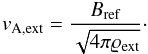 (8)If the timescale for the Alfvén waves to reach the background medium far away from the disk is much smaller than the dynamical evolution timescale of the disk, then the rate of angular momentum flux per unit radian through an annulus at radius rref of thickness drref is
 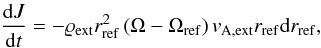 (9)where J denotes angular momentum per radian. The minus sign implies that we assume (Ω − Ωref) > 0, and so angular momentum is lost from the disk. In this expression we do not take into account any azimuthal drift of the field lines with respect to the neutrals, and leave that for a future study. The radius rref, far above the disk where the magnetic field has reached its uniform background state, is threaded by the same field line as radius r in the disk. Equation (9) considers the angular momentum that a volume of gas of mass far away from the disk can take on. Angular momentum flux is calculated by multiplying the angular momentum density ϱΩr2 with the transport velocity vA,ext (which is constant far from the disk).
We perform transformations to express Eq. (9) in terms of quantities at the disk’s surface instead of the external medium. First, we replace the external density by the Alfvén speed in Eq. (8). Another assumption is that magnetic flux Φ, defined by Eq. (7c), is conserved above the disk (flux freezing). Then, we can equate the flux in equatorial plane of the disk  with its value far above the disk, where the magnetic field Bref is uniform. The foot point r in the disk maps to a radius rref above, since the two are connected by a flux tube. We have rref > r because the field lines are extending (diverging) above the disk. This means
 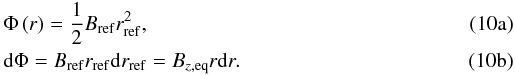 Using these relations, we can rewrite Eq. (9) to yield the angular momentum flux
 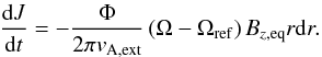 (11)Finally, taking into account the flux in both directions, above and below the disk (yielding a factor of 2), and switching to angular momentum per unit area L ≡ ΣnΩr2 = J/rdr, we arrive at an expression for Ncl, the torque acting on the cloud
 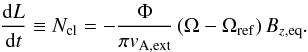 (12)At the same time, the stress-energy tensor yields the change in angular momentum to be equal to rBz,eqBϕ,Z/2π, which allows us to calculate the ϕ-component of the magnetic field at the upper surface of the disk as
 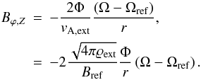 (13)Equation (13) is used in the second term on the right hand side of the equation of angular momentum, Eq. (1c). In the absence of magnetic braking, angular momentum is conserved and this term vanishes.
4. Non-ideal MHD treatment
We outline the derivation of the induction equation with all non-ideal MHD effects: ambipolar diffusion, Ohmic dissipation, and the Hall effect. For brevity and clarity, we only consider a single grain size and omit inelastic collisions. However, we include their effect in our calculations, and refer the interested reader to the detailed exposition in Appendix B.1 in Kunz & Mouschovias (2009) where all terms are included.
We start with Faraday’s law in cgs units, transformed to the frame of the neutrals: 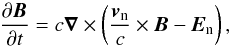 (14)where B is the magnetic field, En is the electric field in the reference frame of the neutrals, vn is the velocity of the neutrals, and c is the speed of light. In ideal MHD, En ≡ 0 by definition, as the conductivity is infinite and so all local electric fields (in the neutral frame) are shorted by currents immediately. This is not the case in non-ideal MHD, where En ≠ 0. We therefore seek an expression for En in the general case.
We take the force equations for all charged species (denoted by subscript s, where in our discussion s = {i,e,g + ,g − }, but others would be possible), assuming force balance between the Lorentz force and collisions with neutrals. Inertial forces and collisions with other charged particles are neglected, as we are working under the assumption of a weakly-ionized plasma (with an ionization fraction χ ≈ 10-8). Then we have 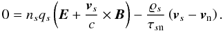 (15)The time scale for collisions between species s and neutrals is given by τsn. The mass density of the charged species is ϱs, while qs is their charge number. Note that the latter carries a minus sign if the charge is negative (e.g., for electrons).
Introducing the drift velocity ws = (vs − vn), we can transform Eq. (15) to the reference frame of the neutrals: 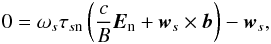 (16)where b ≡ B/B is the unit vector in the direction of the magnetic field, and B ≡ |B| is the magnetic field strength. Also, we have introduced the cyclotron frequency (in cgs units)
 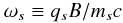 (17)where ms is the mass of the charged particle, and note that ϱs ≡ msns where ns is the number density of the charged species s.
We eliminate the term ∝  by inserting Eq. (16) × b back into Eq. (16). This yields
 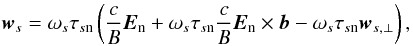 (18)which provides the drift velocity in terms of the electric field in the frame of the neutrals.
First, we look at the component parallel to b: 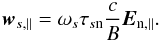 (19)We write the electric current density using the overall charge neutrality ∑ snsqs ≡ 0:
 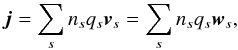 (20)and arrive at a generalized Ohm’s law for the parallel component of j:
 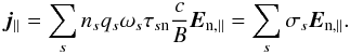 (21)Here,
 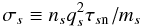 (22)is the conductivity due to species s. Lastly, we define σ∥ = ∑ sσs as well as η∥ = 1/σ∥ and invert Eq. (21) to get
 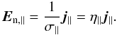 (23)Similarly, we seek a relation between the perpendicular components of electric current density and electric field. Again, we start from Eq. (18), but this time look at the perpendicular component:
 ![Mathematical equation: \begin{eqnarray} \vec{w}_{s,\perp} = \left(\frac{\omega _{s}\tau _{s\mathrm{n}}}{1+ \omega _{s}^{2} \tau _{s\mathrm{n}}^{2}} \frac{c}{B} \right) \left[\vec{E}_{\mathrm{n},\perp} + \omega _{s}\tau _{s\mathrm{n}} \vec{E}_{\mathrm{n}}\times\vec{b} \right]. \end{eqnarray}](/articles/aa/full_html/2012/05/aa17876-11/aa17876-11-eq139.png) (24)Inserting this into Eq. (20), we find
(24)Inserting this into Eq. (20), we find 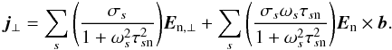 (25)Defining
 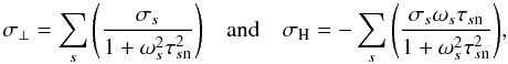 Ohm’s law for the perpendicular component is
 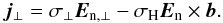 (26)Combining both parallel and perpendicular components, we can write down a generalized Ohm’s law. Note that the magnetic field introduces an asymmetry (and thus off-diagonal components) and makes a tensor expression necessary:
 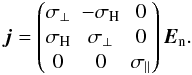 (27)Finally, we invert the matrix to get an expression for the electric field in the reference frame of the neutrals,
  (28)where
 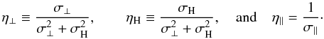 The purely vertical magnetic field in our thin disk is generated by an azimuthal current only. This means that there is no component of the electric current density parallel to the field (and neither in radial direction). Hence we are only interested in the perpendicular component of the electric field, and for convenience quote its expression:
 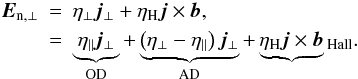 (29)Note that the quantity η ⊥ contains the effects of both ambipolar diffusion and Ohmic dissipation. In Eq. (29), the contributions of each of the three non-ideal MHD effects – Ohmic dissipation (“OD”), ambipolar diffusion (“AD”), and the Hall effect (“Hall”) – are highlighted. We do not consider the Hall effect in the present work.
Summarizing the above derivation, we can write Eq. (14) as 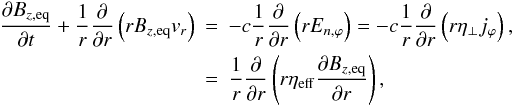 (30)where the relation j = (c/4π)∇ × B has been used, and ηeff ≡ η ⊥ c2/4π was introduced.
5. Chemistry
In this section, we present the chemical model used to calculate the ionization fraction, fractional abundances, and resistivities for seven species. In our models using an MRN grain-size distribution there are a total of 19 species, but we omit the corresponding full chemical model (which can be found in Kunz & Mouschovias 2009) for sake of clarity. In the following, we consider neutral matter (one helium atom per five H2 molecules), atomic and molecular ions (such as Mg+ or HCO+), electrons, and grains (of uniform size, positively-charged, neutral, and negatively-charged). Multiply-charged grains are neglected, because the capture rate by a charged grain of a gas-phase particle with the same charge q is reduced by a factor exp(−q2/akBT) (Spitzer 1941), where a is the particle’s radius. A grain is thus far more likely neutralized by capturing a particle of opposite charge than elevated to higher charge by capturing a particle of the same charge. For example, Nakano et al. (2002) show that the abundance of doubly-charged grains is 5 orders of magnitude less than that of singly-charged ones. We also ignore multiply-charged ions and molecules.
5.1. Ionization rate
We consider four sources of ionization:
-
1.
UV ionization;
-
2.
cosmic ray ionization;
-
3.
ionization due to radiation liberated in radioactive decay;
-
4.
thermal ionization through collisions.
UV ionization is only important where the visual extinction AV ≲ 10 (Ciolek & Mouschovias 1995) or, equivalently, the H2 column density NH2 ≲ 2 × 1022 cm-2. The part of the cloud relevant to this work is much denser (in fact, everything within 104 AU from the center is denser) and, to good approximation, UV ionization would not need to be considered. We still include its contribution in parametrized form, by adding  (see Fiedler & Mouschovias 1992) to the electron and ion number densities. This has the effect to maintain an ionization fraction of ≈ 3 × 10⁻⁵ in the outermost envelope of the core, and keep it flux-frozen, but does not affect the dynamical evolution of higher-density regions.
In the higher-density regions (where 104 cm-3 ≲ nH2 ≲ 1012 cm-3), the ionization is mainly due to cosmic rays. Their ionization rate is calculated by ![Mathematical equation: \begin{equation} \zeta _{\mathrm{CR}} = \zeta _{0} \exp{\left[ - \Sigma _{\mathrm{H _{2}}}\right/96~\mathrm{g}~\mathrm{cm}^{-2}\left. \right]} \label{eq:CR_ion_rate} \end{equation}](/articles/aa/full_html/2012/05/aa17876-11/aa17876-11-eq163.png) (31)(Umebayashi & Nakano 1980), where ζ0 = 5 × 10-17 s-1 is the canonical unshielded cosmic-ray ionization rate (Spitzer 1978).
(31)(Umebayashi & Nakano 1980), where ζ0 = 5 × 10-17 s-1 is the canonical unshielded cosmic-ray ionization rate (Spitzer 1978).
Beyond nH2 ≳ 1012 cm-3, even cosmic rays are shielded and cannot penetrate deeply. Here, radioactivity, mainly due to 40K, still provides a background level of ionization. The ionization rate is ζ40 = 2.43 × 10⁻²³ s-1 (e.g., Kunz & Mouschovias 2009). Other radionuclides (such as 26Al) are not considered, due to their low abundance, their short half-life time, their low ionization rate, or a combination thereof.
Finally, when the temperature reaches ≳ 1000 K, collisions are energetic enough to cause thermal ionization of some atoms with low ionization potential (predominantly potassium). As the temperature rises further, collisions becomes the dominant source of ionization. We parametrize this as an additional source term in the ion equilibrium equation (see Sect. 5.2) with the value (see Pneuman & Mitchell 1965)  (32)where nA0 is the fractional abundance of the neutral atomic particles. The fact that potassium only makes up ≈ 1/14 of all metals (Lequeux 1975) has been considered in the coefficient in front.
Beyond nH2 ≳ 1018 cm-3, at a temperature of ≳ 1500 K, we assume the grains to be destroyed and the stored charges are released into the gas. The gas becomes highly ionized, and we thus revert back to flux freezing (Pneuman & Mitchell 1965). Note that the resistivity has already decreased significantly at this temperature as a consequence of thermal ionization.
5.2. Fractional abundances
In order to calculate the resistivity (see Sect. 4), we calculate the fractional abundance of each species using a chemical equilibrium network.
The molecular ion equation describes the production of molecular ions (such as HCO + ) by radiative ionization, their destruction through charge-exchange reactions with neutral atoms and grains, as well as recombination reactions with electrons:  (33)Here β is the charge-exchange coefficient and αdr is the dissociative recombination rate (collisions with electrons). Their value and that of the other rate coefficients between species s and s′, αs,s′, depend on temperature and grain properties, and are given in Appendix B. The symbol ns refers to the number density of species s. Cosmic rays will ionize molecular hydrogen, forming
  almost instantaneously; this in turn is highly reactive and will strip away an electron from any (non-H2) molecule it encounters. For instance, CO will be transformed to HCO + and H2. This is why cosmic rays act on H2 in the first term of this equation.
Atomic ions (e.g., Na + ) are produced by charge exchange reactions with neutral atoms, as well as thermal ionization, while they are destroyed by radiative recombinations with electrons, and by the collision with grains: 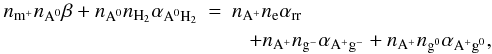 (34)where αrr is the radiative recombination rate, and the second term on the left-hand side represents thermal ionization (see Sect. 5.1).
The equation for positively-charged grains balances the deposition of charge from atomic and molecular ions with the capture of electrons and neutralization with negatively-charged grains. The charge exchange between positively-charged and neutral grains is in steady-state, and so their contribution appears on both sides of the equation and cancels:  (35)Similarly, negatively-charged grains form by capture of an electron by a neutral grain, and are neutralized by charge exchange during collisions with molecular and atomic ions as well as positively-charged grains. Again, the charge exchange between negatively-charged and neutral grains is in steady-state, and so does not appear:
  (36)Finally, to close the system, we include equations for the total number of atoms and grains
 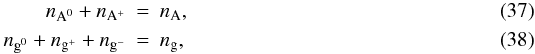 as well as for overall charge neutrality
  (39)Equations (33)–(39) form the non-linear system to be solved for the fractional abundances; we do this iteratively for each time step and each grid point using Newton’s method. The linearized matrix equation that results involves the Jacobian and the update vector to the abundances, and is solved directly using a LU-decomposition package. We assume the mean mass of the molecular and atomic species to be mm + = 29 mp and mA + = 23.5 mp, respectively, where mp is the proton mass. Those values are the masses of HCO + and the average of atomic magnesium and sodium, respectively, which are good representatives of the broader range of species present.
6. Initial conditions and physical units
We assume that our initial state was reached by core contraction preferentially along magnetic field lines (e.g., Fiedler & Mouschovias 1993) and rotational flattening, and prescribe initial profiles for column density and angular velocity given by 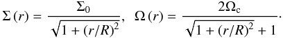 (40)Here, R ≈ 1500 AU approximately equals the Jeans length at the core’s initial central density (see below). The column density profile is representative of the early stage of collapse (e.g., Basu 1997; Dapp & Basu 2009), and the angular velocity profile reflects that the specific angular momentum of any parcel is proportional to the enclosed mass mencl.
We assume an initial profile for Bz,eq such that initially the normalized mass-to-flux ratio  everywhere, which is the approximate starting point of runaway collapse (e.g., Basu & Mouschovias 1995), and also consistent with observed values in molecular cloud cores (Crutcher 1999). The core is at rest at the beginning of our simulations, i.e., the radial velocity is zero. The initial state is not far from equilibrium, as the pressure gradient and magnetic and centrifugal forces add up to ≈ 82% of the gravitational force. Our results do not depend strongly on the choice of initial state, as long as gravity remains dominant.
The initial central column density is set to Σ0 = 2 × 10⁻² g cm-2. The core has a temperature T = 10 K, and its total mass and radius are 28.5 M⊙ and 0.6 pc, respectively. The initial central number density and magnetic field strength are nc = 3.3 × 104 cm-3 and Bz,eq ≈ 200 μG, respectively. We choose the external density to be next = 103 cm-3, and the central angular velocity Ωc such that the cloud’s edge rotates at a speed of 0.1 km s-1 pc-1.
Transient adjustments occur if the simulation is started from an initial non-equilibrium state that is at rest. The chemistry calculations are quite sensitive to fluctuations in density, which can cause problems. We therefore let the system evolve from an initial state with the above-mentioned profiles and characteristics, but initially without non-ideal MHD effects. Once the cloud has settled into a steady infall (at a central density of approximately nc ≈ 4 × 106 cm-3) the full MHD equations Eqs. (1a)–(1e) are solved. The state at which we switch on the detailed treatment of chemistry corresponds very closely to the initial state employed by DB10, so that comparisons with their results are possible. The rotation rate by then has increased to 1 km s-1 pc-1, consistent with observations of large molecular cloud cores (Goodman et al. 1993; Caselli et al. 2002). In the plots in this paper, we show only the region of the core within 0.05 pc, again consistent with DB10. Note that the nature of the collapse is very dynamical and happens under flux freezing to a very good approximation between nc ~ 104 − 1010 cm-3 (see Kunz & Mouschovias 2010).
We fix the dust-to-gas ratio at 1%, consistent with observations (Spitzer 1978), and keep it constant everywhere and at all times. This means that a different mean grain size agr will result in differing total numbers of grains available, scaling as  , with a total surface area ∝
  .
.
7. Results
7.1. Collapse phase
We ran multiple models with different single grain sizes, and one with a standard “MRN” distribution (named after its authors: Mathis, Rumpl, & Nordsieck 1977). In this case, the number density of spherical dust grains with radii between a and a + da is  (41)The distribution is truncated at a lower grain radius amin = 0.011 μm and an upper grain radius amax = 0.26 μm. The coefficient NMRN is proportional to the dust-to-gas mass ratio in the cloud. Kunz & Mouschovias (2009) found that there is reasonable convergence for 5 grain size bins, so we choose that number in order to limit computational expense. More detail can be found in that paper (their Sect. 4.2). Our models are summarized in Table 1.
Simulation model overview.
Figure 1 shows the column number density profile versus radius at different times for Model 2 (with agr = 0.038 μm). Several features are identifiable via their associated breaks in the profile. From the outside in, those are:
-
1.
Prestellar infall profile withN ∝ r-1. This corresponds to a volume number density profile of n ∝ r-2, typical for collapsing cores dominated by gravity (see, e.g., Larson 1969; Dapp & Basu 2009). The vertical hydrostatic condition mandates that n ∝ N2.
-
2.
At ≈ 10 AU, a magnetic wall (Li & McKee 1996; Contopoulos et al. 1998; Tassis & Mouschovias 2007). Here, the relatively well-coupled, bunched-up magnetic field expelled (relative to the neutrals) from the first core decelerates material temporarily. At smaller radii, the infall continues.
-
3.
Expansion wave profile with N ∝ r − 1/2 outside the first core. The power law can be motivated analytically (see Shu 1992, for the spherical case). Energy conservation requires the infall speed from large distances towards a point mass (i.e., the first core) with mass M to scale as
 . At the same time the infall onto the point mass is essentially a steady-state process, and thus Ṁ ≡ 2πrΣvr = const., close to the border of the first core. Together, those two relations imply Σ ∝ r − 1/2. item First core at 1 AU. Here, the density is sufficiently high that the gravitational energy released in the collapse cannot escape as radiation anymore. The temperature rises, and thermal pressure gradient stabilizes the object. The first core starts nearly in hydrostatic equilibrium, and its radial and vertical extent are approximately equal.
 -
4.
Infall profile onto the second core with N ∝ r-1. After the temperature in the first core has reached ≈ 1000 K, hydrogen dissociates. This process provides a heat sink, and the temperature no longer increases sufficiently for thermal pressure to balance gravity. The core starts to collapse again and flattens at the same time.
-
5.
Beginning expansion wave profile with N ∝ r − 1/2 outside the second core, for the same reasons as outside the first core. Once this rarefaction wave reaches the boundary of the first core, the material comprising the first core will fall in to a region of stellar dimensions, unless it forms a centrifugal disk.
-
6.
Second core at ≈ 1 R⊙. After hydrogen dissociation (and ionization) has concluded, the temperature rises again, and a truly hydrostatic object, the YSO, is formed. It is also partly supported by electron degeneracy pressure (Masunaga & Inutsuka 2000).
Figure 2 shows the evolution of the central diffusion coefficient ηeff versus number density for the various models (different single grain sizes and the MRN distribution of grain sizes; see Table 1), as well as the parametrized resistivity used in Machida et al. (2006) and DB10. At low densities, electrons and ions are the dominant (but not exclusive) contributors to the conductivity. Smaller grains are fairly well coupled to the magnetic field because of their smaller gyro-radii and smaller collisional cross sections, so their contribution to the effective resistivity is lower than that of larger grains. However, there is a competing effect: smaller grains have an increased capability to absorb gas-phase charge carriers because of their larger total surface area. For grains with radius agr = 0.075 μm (dot-dashed line) and larger, the trend reverses and the conductivity increases (the resistivity decreases) with larger grain radius, as expected from an increased ionization fraction.
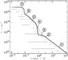 |
Fig. 1 Column number density profile versus radius for Model 2. The thin lines (in ascending order) are plots at the times listed in Table 2. Several features are identifiable via their associated breaks in the profile. (1) Prestellar infall profile with N ∝ r-1. (2) Magnetic wall at ≈10 AU, where the bunched-up field lines decelerate material before it continues the infall. (3) Expansion wave profile with N ∝ r−1/2 outside the first core. (4) First core at 1 AU. (5) Infall profile onto the second core with N ∝ r-1. After the first core has reached ≈1000 K, it starts to collapse, as H2 is dissociated. (6) Expansion wave profile with N ∝ r−1/2 outside the second core. (7) Second core at ≈1 R⊙. |
This effect is demonstrated in Fig. 3 which shows the diffusion coefficient versus grain size at two densities (n ≈ 107 cm-3 – solid line; n ≈ 1015 cm-3 – dashed line). The symbols indicate values for which we have complete runs, while the continuous lines are computed by calculating the effective resistivity with values for temperature, column and volume density, as well as magnetic field averaged over the values from the available complete runs. The magnetic field strength enters the resistivity only though the gyro-frequency, and the estimated error in the continuous lines is typically <1%. The diffusion coefficient takes on a maximum at a grain size of agr ≈ 0.065 μm for low densities (solid line in Fig. 3). As described above, for grains with smaller radius, the effect of better coupling dominates, while at larger grain sizes, the associated decrease in total surface area leaves more free gas-phase charges, and makes for a higher conductivity, and conversely a decreased resistivity.
At intermediate densities the resistivity in Fig. 2 rises sharply, as a consequence of the grains soaking up gas-phase charges and decoupling from the magnetic field. Additionally, the conductivity drops because at high column density cosmic rays are shielded according to Eq. (31). At nc ≈ 1013 cm-3 the only remaining source of ionization is radioactivity, which provides a floor ionization rate (see Sect. 5.1). At this stage, clearly distinguished by a break in the profile, the resistivity is almost exclusively due to grains, i.e., their collisions with neutrals. Inserting Eq. (A.1) of Appendix A into Eq. (22), we see that conductivity scales as  in this phase. The resistivity is the inverse of the conductivity, and hence it increases with larger grains as a consequence of their lower gyro-frequencies and greater collision cross sections. This happens even though there are fewer grains with increasing grain size, and they have a reduced total surface area. The dashed line in Fig. 3 shows this monotonic increase in diffusion coefficient with grain radius at a central density of nc ≈ 1015 cm-3. As the temperature approaches ≈1000 K, collisions become energetic enough that thermal ionization occurs, described by Eq. (32). The conductivity recovers, and hence the resistivity decreases again. Finally, during the second collapse, as temperatures of ≈ 1500 K are reached, grains are destroyed and all locked-up charges are released into the gas phase. Electrons and ions flood the gas, the ionization fraction rises sharply, and flux-freezing is restored (see Sect. 5.1). We switch off the chemistry calculations at this point, shown by the right vertical dashed line in Fig. 2). We point out that the parametrization for only Ohmic dissipation used in Machida et al. (2006, 2007) and DB10 (for comparison shown in Fig. 2 as the dotted line) yields values for the resistivity lower by at least a factor of 10 everywhere.
In Model 9 (the MRN distribution), the diffusion coefficient is dominated by the smallest grain size present, and behaves otherwise very similar to the simulations with a single (small) constant grain size.
Note that Fig. 2 shows data extracted from the central cell of a dynamical simulation. The exact value of the diffusion coefficient not only depends on the grain size and the local number density of the neutrals, but also on the number densities of the other species and the local values of magnetic field strength, temperature, and column density. As a result, the values shown in this plot are not necessarily representative of any other point in the cloud. It is therefore not helpful to parametrize the diffusion coefficient according to this plot and simply use an approximate interpolative expression as a replacement for a realistic calculation of the microphysics and ionization balance. The procedure outlined in Sects. 4 and 5 is the simplest method of obtaining accurate values for the diffusion coefficient.
Figure 4 shows the relative contribution of ambipolar diffusion (AD) and Ohmic dissipation (OD) to the resistivity coefficient near the end of the run. The coefficient is determined mainly by AD everywhere outside the first core at r ≈ 1 AU. In fact, AD dominates OD up to a density of nc ≈ 5 × 1012 cm-3. The contribution of OD continues to increase sharply at higher densities and is the dominant non-ideal MHD effect within the first core. Its coefficient only decreases again in the vicinity of the second core at ≈ 0.1 AU, where thermal ionization drives up the conductivity. Note that the comparatively large AD diffusion coefficient outside ≈ 102 AU does not cause a large flux loss since the dynamical time is still much smaller than the diffusion time associated with AD.
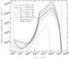 |
Fig. 2 Central diffusion coefficient ηeff versus number density for different grain sizes, extracted from the dynamical model. The vertical line at the left indicates the density at which the detailed chemistry and non-ideal MHD treatment is switched on. Beyond nc ≈ 1018 cm-3 the resistivity plummets, after having already declined due to thermal ionization. This is where we switch the chemistry calculations off again, and is denoted by the vertical line on the right. Due to grain destruction, flux-freezing is restored there. |
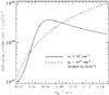 |
Fig. 3 Diffusion coefficient versus grain size for two values of number density. The diffusion coefficient behaves qualitatively differently at different densities. While at high densities, the diffusion coefficient increases monotonically with increasing grain radius, it has a maximum for low densities at a grain size of agr ≈ 0.065 μm. Below this radius, the effect of better coupling dominates, while at larger grain sizes the decreased surface area of the larger grains leaves more free gas-phase charges, with associated higher conductivity, and conversely decreased resistivity. |
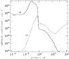 |
Fig. 4 Contributions due to ambipolar diffusion (AD) and Ohmic dissipation (OD) to the effective resistivity in Model 2 (grain size agr = 0.038 μm) at the end of the run. OD only dominates AD beyond nc ≈ 1012 cm-3, within the first core. |
In Figs. 5 and 6 we present the evolution of the central ionization fraction versus number density for the different models, and the abundances of grains and gas-phase species relative to molecular hydrogen. Figure 5 shows that at low densities the smaller grains result in a lower ionization fraction. The reason is that small grains are highly abundant and thus have a large surface area to which the gas-phase charges can adhere. An increasing density causes the ionization fraction to decrease with a slope slightly steeper than the canonical relation ∝  for cosmic-ray-dominated ionization. At intermediate densities the decrease in ionization fractions level off, starting at the lowest density for the smallest grains and at progressively higher densities for successively larger grains. This phenomenon is driven by the electrons adsorbing to the grains. The ions also adsorb to the grains, but due to a lower thermal speed than the electrons, their collision rate is much smaller. With the grains acting as a reservoir for charges, and cosmic-ray ionization continuing to be active, the decrease in ionization fraction is temporarily halted. This occurs at later stages with increasing grain size, as Fig. 6 shows, for the reason of the lower overall grain abundance (scaling as ), which cannot be compensated by a larger collision rate (see Eq. (B.7) in Appendix B). Beyond nc ≳ 1012 cm-3, the ionization fraction in Fig. 5 drops precipitously for all grain sizes, as cosmic rays become shielded due to high column densities. The evolution at still higher densities is determined by radioactivity, until finally thermal ionization kicks in at nc ≈ 1016 cm-3. Potassium is one of the first species to be ionized, but as the temperature increases further, grain evaporation also releases charges into the gas.
Figure 7 compares the mass-to-flux ratio (normalized to the value critical for collapse) for the various models at the time thermal ionization reestablishes flux freezing, when nc ≳ 1019 cm-3, shortly before the formation of a central protostar. For comparison, we also show the mass-to-flux ratio for a model with flux-freezing throughout, and the model with only the simple prescription for Ohmic dissipation used in DB10. The inclusion of ambipolar diffusion and the more realistic treatment of the microphysics lead to a further weakening of the magnetic field, both in the first core (by a factor of ≈ 102), and in the region outside (by a factor of ≈ 2). The region with increased mass-to-flux ratio also extends out slightly further, also by a factor of ≈ 2. This is caused by the higher effective value of the resistivity and the earlier onset of its efficacy. The mass-to-flux ratio increases by a factor of ≈ 104 over the course of the evolution, to ≈ 20 000 times the critical value. Field strengths in main-sequence stars and T-Tauri stars require flux reduction of a factor ≈ 104 − 108 (even if their field is dynamo-generated) if their parent molecular clouds are assembled from subcritical μ < 1 atomic gas. This is known as the “magnetic flux problem” of star formation. Our results constitute substantial progress towards understanding its resolution.
 |
Fig. 5 Total ionization fraction versus central density for different grain sizes. The vertical line indicates the density at which the detailed chemistry and non-ideal MHD treatment is switched on. |
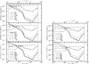 |
Fig. 6 Central fractional abundances of species. Top left: Model 1, agr = 0.019 μm, middle left: Model 2, agr = 0.038 μm, bottom left: Model 3, agr = 0.075 μm. The convergence of the abundances of positively- and negatively-charged grains is pushed to higher densities with increasing grain radius. The departure of the electron abundance from the ion abundance also happens at higher densities with decreasing grain surface area. The dashed vertical line at nc ≈ 106 cm-3 indicates the density at which the chemistry and non-ideal MHD treatment are switched on, while the one at nc ≈ 3 × 1018 cm-3 shows when we assume the destruction of grains restores flux-freezing. Top right: Model 4, agr = 0.113 μm, bottom right: Model 5, agr = 0.150 μm. Since the grain radius increases only by a factor of 4/3 from Model 4, the effect on the abundances is less pronounced than it was for the smaller grains. |
Output timesa and corresponding central number density in the profile plots.
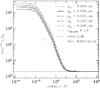 |
Fig. 7 Mass-to-flux ratio μ versus radius for different grain sizes at the time of the formation of the second core. For comparison, the thin dashed line shows the case with only the simplified version of Ohmic dissipation, as used in DB10. In the center, the difference is a factor of ≈ 102, but further out it it still 2 × higher, and also shows a greater extent by about this factor. The reason is twofold: firstly, ambipolar diffusion is important at lower densities and, secondly, the effective resistivity is larger everywhere than the parametrization used in DB10 (cf. Fig. 2). |
Figure 8 shows the evolution of the radial profile of the vertical component of the magnetic field. At low densities, Bz increases under near flux freezing. Ambipolar diffusion is present and active, but is too slow to be dynamically important. Dramatic flux loss occurs once grains become the dominant charge carriers at n ≈ 1011 cm-3 and the field evolution slows. This can be seen in the bunching-up of the thin lines that are snapshots at different times (at constant increments of number density, at times given in Table 2). The small fluctuations near the interface of the first core result from differentiating ηeff and taking a second derivative of Bz in the induction equation. Near the interface of the first core, the steep dependence of ηeff on density in the range 1011 cm-3 < n < 1013 cm-3 (see Fig. 3) combined with an extreme gradient of the density, cause a jump in the diffusion coefficient of many orders of magnitude.
We stress that these fluctuations are not numerical instabilities and do not grow with time. The implicit, adaptive ODE solver we use to solve the MHD equations with the method of lines (see Sect. 2) is unconditionally stable.
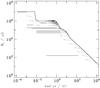 |
Fig. 8 Evolution of Bz versus radius over time. The thin lines are plots at the times listed in Table 2, for the fiducial grain radius of agr = 0.038 μm. |
In Fig. 9 we present the profile of the angular velocity at various times. At large radii, Ω ∝ r-1 because the core evolves under near angular momentum conservation with the specific angular momentum j ≡ Ωr2 ∝ mencl and Σ ∝ r-1 in the prestellar infall (cf. Fig. 1). Inside the expansion wave, there is a break in the angular velocity profile, as expected from theoretical considerations (e.g., Saigo & Hanawa 1998). The enclosed mass in that region is essentially the mass of the first core (the expansion wave itself does not contribute much), and so is approximately constant with radius. Then j ∝ mencl ≈ const, and therefore Ω ∝ r-2.
The radial velocity (Fig. 10) shows the first and second cores very clearly. At their edges (≈1 AU and ≈10-2 AU = 2 R⊙, respectively), accretion shocks develop and the velocity drops precipitously. Outside the cores, in the expansion wave, the velocity follows a power law ∝ r − 1/2. At ≈10 AU, a slight bump in the infall velocity hints at the magnetic wall. The fluctuations within the first and second cores stem from the fact that we plot absolute values in a log-log plot: in nearly-stable conditions as prevalent there, the velocity can be positive or negative, but remains small.
 |
Fig. 9 Evolution of the angular velocity Ω versus radius over time. The thin lines are plots at the times listed in Table 2, for the fiducial grain radius of agr = 0.038 μm. The profile changes from being ∝ r-1 to ∝ r-2 in the expansion wave, as expected from theoretical considerations. |
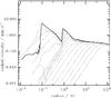 |
Fig. 10 Evolution of the infall radial velocity |vr| versus radius over time. The thin lines are plots at the times listed in Table 2, for the fiducial grain radius of agr = 0.038 μm. Outside the first core, the magnetic wall causes a small bump. Within the first and second cores material is moving about inwards and outwards with small speeds. This causes spikes when absolute values are plotted on double-logarithmic axes. |
7.2. Disk formation
The second core is a truly hydrostatic object, and very nearly spherical, and so the thin-disk approximation breaks down there. Therefore, once the central number density nc ≈ 1020 cm-3, we introduce a sink cell of radius ≈3 R⊙. Note that this is two orders of magnitude smaller than is commonly used (e.g., Mellon & Li 2008, 2009).
In Fig. 11 we present evidence for the formation of a centrifugal disk. The figure shows the profiles of column density, infall velocity, and the ratio of centrifugal to gravitational acceleration shortly after the introduction of the sink cell. This is done for Model 2, which has resistivity and the fiducial grain size agr = 0.038 μm, and for a model without resistivity. In the resistive model, centrifugal balance is achieved in a small region (≈10 R⊙) close to the center (bottom panel), while the flux-freezing model is braked “catastrophically”, and the support drops to minuscule values. Centrifugal balance is a necessary and sufficient condition for the formation of a bona-fide centrifugally-supported disk (as opposed to a larger flattened structure that is still infalling). At the same time all infall is halted there and the radial velocity plummets (middle panel), while in the flux-freezing model infall continues unhindered. After a few more months of evolution, a Toomre instability develops, and the rotationally-supported structure breaks up into a ring (top panel, solid line). At this point, we stop the simulation, because more physics would be required to follow the further evolution of the disk.
DB10 also presented a model without magnetic braking (their Fig. 1). In that case, the entire first core turns into a large centrifugally-supported structure of size several AU.
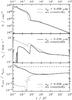 |
Fig. 11 Evidence for disk formation. Top panel: column density profile. The system is Toomre-unstable, and breaks up into a ring in the resistive model (solid line), but not in the flux-frozen model (dotted line). Middle panel: infall profile. Infall is stopped in the resistive model (solid line), in innermost region where a centrifugal disk forms, but not in the flux-frozen model (dotted line). Bottom panel: ratio of centrifugal over gravitational acceleration. In the resistive model, centrifugal balance is achieved. In contrast, catastrophic magnetic braking occurs for the flux-frozen model, the centrifugal support drops to negligible values and the first core is spun down drastically. |
Figure 12 shows the magnetic field line topology above and below the disk on two scales (10 AU and 100 AU) for both the flux-freezing and non-ideal MHD models. The field lines are calculated shortly after the formation of the second core, assuming force-free and current-free conditions above a finite thin disk (Mestel & Ray 1985). The split monopole of the flux-frozen model (dashed lines) is created as field lines are dragged in by the freely falling material within the expansion wave front at ≈15 AU. This is replaced by a more relaxed field line structure in the non-ideal case (solid lines), for which the field is almost straight in the central region. Galli et al. (2009) presented similar field configurations resulting from a simplified model for Ohmic dissipation during the collapse. The extreme flaring of field lines in the flux-freezing model is a fundamental cause of the magnetic braking catastrophe.
We can estimate the efficiency of magnetic braking by comparing its instantaneous timescale with that of the dynamical evolution of the core. The relevant ratio is  (42)where L = ΣΩr2 is the angular momentum per unit area, Ncl = rBϕBz/2π is the torque per unit area acting on the cloud, and τdyn = r/vr is the dynamical time. Figure 13 shows this ratio for catastrophic magnetic braking for our cloud after the second core has formed. In the region of dynamical collapse still characterized by a prestellar infall profile, magnetic braking is not very effective (its time scale being ≈3 times that of dynamic evolution) and the cloud evolves under approximate angular momentum conservation. In the non-ideal MHD case (solid line), the magnetic braking time is never shorter than the dynamical time, and thus catastrophic magnetic braking is avoided. However, the ratio comes close to unity in the expansion wave where a significant amount of angular momentum loss can still occur. Within the first core however, where the magnetic field has been weakened by diffusive effects, magnetic braking is totally disabled, and the ratio τMB/τdyn rises dramatically. For flux freezing (dashed line), the ratio drops below unity within the expansion wave, and the first core marks a further sharp drop in the magnetic braking time to only a tenth of the dynamical time. Both the decline of τMB/τdyn within the expansion wave as well as its sharp drop within the first core can be considered elements of catastrophic magnetic braking.
 |
Fig. 12 Magnetic field lines. The box on the left has dimensions 10 AU on each side, while the box on the right has dimensions 100 AU. The dashed lines represent the flux-freezing model, while the solid lines show the same field lines for the model including non-ideal MHD effects for a grain size agr = 0.038 μm. In both cases, the second core has just formed and is on the left axis midplane. The field lines straighten out significantly on small scales in the non-ideal model compared to the flux-frozen model. |
Scaling laws in the flux-freezing case.
In the flux-freezing case (where the magnetic field eventually forms essentially a split-monopole configuration, dashed line of Fig. 12), simple analytic scaling arguments can be made to explain the profiles. These are summarized in Table 3. The vertical component of the magnetic field, Bz, always scales like the column density Σ due to the spatially constant mass-to-flux ratio, and magnetic flux conservation (flux-freezing), while Br scales like the gravitational field. The azimuthal component of the magnetic field, Bϕ ∝ ΦΩr-1 from the magnetic braking calculation (see Sect. 3).
In the prestellar infall region under flux freezing, the magnetic braking time 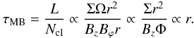 (43)Similarly, the dynamical time in the prestellar profile scales as
 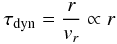 (44)since vr ≈ const. The magnetic braking time and the dynamical time therefore scale with radius in the same way; in other words their ratio is constant.
In the expansion wave region, the enclosed flux is dominated by the split-monopole, and is approximately constant (similar arguments hold for the enclosed mass). Furthermore, Σ, Bz, and vr scale differently than in the region of prestellar infall (see Table 3). Then in the expansion wave region 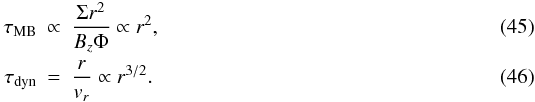 Here, the ratio of magnetic braking time and dynamical time is ∝ r1/2, as seen in Fig. 13 between ≈ 1 AU and ≈ 15 AU (for the dashed line). This shows that the magnetic braking catastrophe is a fundamental property of the expansion wave in a flux-frozen model. In the non-ideal case, the magnetic field does not assume a split-monopole configuration, and neither does the mass-to-flux ratio remain spatially constant, and simple scaling laws are not applicable.
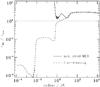 |
Fig. 13 Plot of the ratio τMB/τdyn. For both the flux-freezing case (dashed line) as well for non-ideal MHD (solid line), the magnetic braking time is reduced in the expansion wave region from what is was in the prestellar infall region. In the case of non-ideal MHD, it turns up sharply at the interface of the first core where diffusion has reduced the magnetic field strength significantly and rendered magnetic braking ineffective. In the flux frozen case however, the first core marks a sharp drop in magnetic braking time to only a tenth of the dynamical time. |
The centrifugal radius of a mass shell, i.e., the radius at which the material would achieve centrifugal balance with gravity if angular momentum were conserved, can be estimated according to 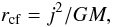 (47)where j = Ωr2 is the specific angular momentum, and M is the mass in the central object. While this expression is strictly true for infall onto a point mass, we take M to be the enclosed mass. The result is shown in Fig. 14. This estimation is imperfect within the first core, but well-justified outside it since the gravitational potential there looks like that of a point mass. At larger radii, most of the enclosed mass is in the cloud and not the central mass, but by the time the expansion wave reaches those mass shells and rapid infall begins, approximately half of the enclosed mass will be in the compact central object or disk (e.g., Shu 1977). The solid line is the estimate based on Eq. (47) but the dotted line takes into account an estimated loss of specific angular momentum j by a factor of 3−4 in the expansion wave, so that j2 is reduced by a factor of 10. This estimate is supported by data presented later in Fig. 17 and is applied to mass shells that are well outside the expansion wave at the time that we stop our simulation. The dotted line may represent an upper limit to the disk radius since some more angular momentum may be lost by magnetic braking when the disk is forming, if magnetic field dissipation has not completely shut off magnetic braking by that time. Future calculations can settle that issue. Outflows will also remove some angular momentum from the forming disk, reducing the size further, although a counter-effect that we do not quantify is disk expansion due to internal angular momentum transfer within the disk. We assume the latter to not be significant in the early Class 0 phase. The dotted line reveals a centrifugal radius rcf ≈ 1 AU for mass shells currently at a distance of 200 AU from the center, and rcf ≈ 10 AU for mass shells at 1500 AU. The upper axis labels the times at which the expansion wave (traveling at the sound speed) is estimated to reach these radii, and rapid infall to begin. The subsequent infall to the disk should take significantly less time than the expansion wave arrival time, since the infall is highly supersonic. Hence, the expansion wave arrival times can be taken to be approximate estimates of the central object age just as the centrifugal radii estimates can be taken to be upper limits to the disk size.
 |
Fig. 14 Estimated centrifugal radius of each mass shell. Beyond ≈ 10 AU, the centrifugal radius increases linearly. The solid line is the current centrifugal radius, while the dotted line is an estimate of rcf after the expansion wave has passed and the associated magnetic braking has reduced the specific angular momentum (see text). The top axis shows the approximate times at which the expansion wave is expected to pass a certain radius. The symbols show the estimated centrifugal radii of 1 AU and 10 AU. The associated times are 6 × 10³ yr and 4 × 10⁴ yr. |
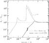 |
Fig. 15 Ratio of Br/Bz,eq. In the flux frozen case (dashed line), Br dominates everywhere within the expansion wave, indicative of extreme flaring and a split-monopole field configuration. With field diffusion active (solid line), the field lines straighten out quickly inside the expansion wave (cf. Fig. 12). |
7.3. Further results
Figure 15 shows the ratio of the radial and vertical components of the magnetic field, Br/Bz,eq. This is a quantitative measure of the local bending of the magnetic field (while Fig. 12 is a visual representation). For flux freezing (dashed line), Br dominates everywhere within the expansion wave, which is indicative of the extremely-flared split-monopole field configuration. Foot points of magnetic flux tubes are connected to head points at much larger radii. This large lever arm leads to rapid angular momentum loss – the magnetic braking catastrophe (Galli et al. 2009). In the diffusive case (solid line), the field lines straighten out quickly inside the expansion wave, and only a small increase in pitch angle occurs inside it.
Again, we can make scaling arguments in the flux freezing case. The radial component of the magnetic field, Br, always scales like the radial gravitational field. In the prestellar region of the profile (outside ≈ 100 AU) Br and Bz both scale ∝ r-1 and so their ratio is constant. In the expansion wave outside the first core (between ≈ 1 AU and ≈ 15 AU) on the other hand, Br ∝ r-2 while Bz ∝ Σ ∝ r − 1/2. Their ratio is therefore ∝ r − 3/2. As before, the magnetic field does not assume a split-monopole configuration in the non-ideal case, and simple scaling laws are therefore not applicable.
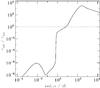 |
Fig. 16 Ratio of diffusion time τdiff and dynamical time τdyn at the end of the run. Within the expansion wave, the ratio is smaller than unity, and diffusion dominates over advection. |
Figure 16 shows the ratio of diffusion time τdiff and dynamical time τdyn near the end of our simulation run. Contopoulos et al. (1998) showed from scaling arguments that upon close approach to the protostar, diffusion of magnetic flux will eventually dominate advection. For our model, this is already the case in the expansion wave outside the first core. The reason for the sudden drop in the ratio at the interface of the first core is that the diffusion time scale τdiff ∝ L2/ηeff, where L is the local scale length. However, not only does the density at this location increase very steeply, ηeff itself increases very steeply in the relevant density range too (see Fig. 2). Though mitigated by a simultaneous decrease in the dynamical time scale (see Fig. 10), it still effects a drop of 5 orders of magnitude in the time scale ratio.
 |
Fig. 17 Specific angular momentum versus enclosed mass at initial state (dashed line) and final snapshot (solid line), and their ratio (dotted line). The expansion wave brings with it a maximal reduction of specific angular momentum. Further insight is provided by the radius versus enclosed mass, plotted as the dot-dashed line, with radius values denoted on the second axis on the right. |
In Fig. 17, we plot the specific angular momentum versus enclosed mass at the initial state (dashed line) and the final snapshot (solid line), as well as their ratio (dotted line). The expansion wave brings with it a maximal reduction (a factor of ≲ 4) of specific angular momentum. The radius versus enclosed mass is plotted as the dot-dashed line. The steep rise of the latter at ≈ 4 × 10⁻³ M⊙ is a consequence of the first core dominating the enclosed mass, and the material within the expansion wave only slowly increasing it at larger radii.
8. Discussion
Our results lead us to propose the following scenario of disk formation and evolution in low-mass stars:
-
1.
A small disk forms, initially ≪ 1 AU, but eventually encompasses the entire first core with ≈ 1 AU, since magnetic diffusion is very efficient there and inactivates magnetic braking.
-
2.
Figure 14 shows that the estimated centrifugal radius of a mass shell at radius ≲ 50 AU lies within ≈ 1 AU. That means that the matter can fall to this radius without hitting a rotational barrier.
-
3.
At the same time, Fig. 13 shows that magnetic braking is active within the expansion wave, while it is dormant in the region of dynamical infall further out. Any material within the expansion wave (which moves outward at the local speed of sound) will lose part of its angular momentum by magnetic braking (typically a factor of 3−4, cf. Fig. 17), and have its centrifugal barrier moved further inward. This is reflected in the dotted line in Fig. 14, which estimates the final centrifugal radius of a mass shell. After the expansion wave passes, material as far as r ≈ 200 AU can directly accumulate onto the inner ≈1 AU. Furthermore, a centrifugal radius ≲10 AU is expected for gas currently within ≈ 1500 AU, which encloses about 0.4 M⊙ in our model. The expansion wave will take ≈4 × 10⁴ yr to reach that point. We therefore predict no disk larger than ≈10 AU to be detectable in Class 0 objects younger than ≈4 × 10⁴ yr. This agrees well with the observations of Maury et al. (2010) who do not find evidence for disks >50 AU in Class 0 objects. ALMA will soon allow observers to test this prediction more stringently.
-
4.
The material in the disk will be subjected to internal mechanisms of angular momentum redistribution, e.g., the MRI (Balbus & Hawley 1991; Balbus 2011), and/or gravitational torques. It is a fair assumption that a disk in which self-gravity is important self-regulates to Q ≈ 1 by such processes (e.g., Vorobyov & Basu 2007). The parameter Q = csΩ/(πGΣ) approximately determines whether a rotating disk is unstable to fragmentation (Toomre 1964; Goldreich & Lynden-Bell 1965). The exact critical value depends on the geometry and the equation of state, but generally spirals and clumps will form if Q ≲ 1, while a situation with Q ≳ 1 is stable (e.g., Gammie 2001).
-
5.
Redistribution of angular momentum allows material in the inner disk to be funneled onto the star, while material further out gains the excess angular momentum and expands its orbit. Basu (1998) showed that internal redistribution of angular momentum means that the disk radius obeys
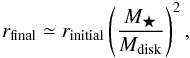 (48)where Mdisk and M★ are the disk and star mass, respectively. This means that the disk will expand by a factor of 102 by the time that 90% of its mass has accreted onto the central object.
 -
6.
By the time the central object has accreted a significant amount of the available material (several 105 yr), a tenuous disk of several hundred AU will be present, consistent with observations (e.g., Andrews & Williams 2005). We expect that the disk will expand due to internal angular momentum redistribution, but that it will occur primarily after the Class 0 phase. During the Class 0 phase, the disk mass may remain a fair fraction of the star mass (Vorobyov 2011), limiting the expansion implied by Eq. (48).
The first step of the above scenario is broadly consistent with the models of Machida & Matsumoto (2011) that have a small initial rotation rate. They have studied disk formation with their three-dimensional models that resolved the second core using a simplified resistivity. However, their models with rotation comparable to observations achieve a very rapidly rotating first core, which evolves directly into a “Keplerian” (their words) disk before the central stellar core has been established. While the term “Keplerian” is normally reserved for when the central point mass dominates the overall gravitational potential, we consider that in their context it refers to centrifugal balance. In fact, we did obtain a similar result in DB10 for a model with no magnetic braking, where the first core formed with rapid rotation that prevented it from collapsing further. In the model of Machida & Matsumoto (2011) a stellar core does eventually form, but is surrounded by a Keplerian disk from the start. Conversely, in our models with an observationally-motivated rotation rate, the sustained effect of magnetic braking throughout the collapse ensures (even in the presence of Ohmic dissipation and ambipolar diffusion) that the first core can undergo rapid infall onto the second core. A centrifugally-supported disk is only built up subsequently through accretion. We start with a differentially-rotating initial state, consistent with prior gravitational collapse (Basu 1997), while Machida & Matsumoto (2011) start with solid body rotation, which puts more angular momentum in the outer regions. The two possible outcomes of direct second collapse followed by disk formation by accretion versus a large centrifugally-supported disk-like first core that coexists with a second core may certainly be a function of the implementation of magnetic braking and non-ideal MHD, initial rotation profiles, and the varieties of dimensionality and boundary conditions of different models. Future modeling can clarify this interesting duality of outcomes in the earliest phase of disk formation.
Previous ideal and non-ideal MHD simulations of protostellar collapse focused on the formation of large centrifugal disks of size ≈ 100 AU. For example, Mellon & Li (2009) and Li et al. (2011) find that the inclusion of ambipolar diffusion, Ohmic dissipation, and even the Hall term are not sufficient to avoid catastrophic magnetic braking at the distances > 7 AU from the origin that they model, for models with realistic initial magnetic field strength. Machida et al. (2011) claim that a disk can finally form in later stages when the envelope is depleted and magnetic coupling to outer moment of inertia is therefore weak. Krasnopolsky et al. (2010) invoked “anomalous” resistivity to weaken the effects of magnetic braking and thereby allow for the formation of large centrifugal disks.
We note that there is no a priori reason why centrifugal disks should be large in the early accretion phase. Using an observationally motivated magnetic-field strength and without recourse to “anomalous” resistivity, we have demonstrated that centrifugal disks can form during the Class 0 stage, albeit not as large as ≈100 AU. Our result is made possible by our resolution of the innermost regions of collapse, and a sufficiently accurate treatment of the relevant chemical and magnetohydrodynamical processes. While not yet computationally feasible, well-resolved three-dimensional simulations that take into consideration these processes would represent a significant advance beyond the thin-disk approximation we have employed here.
The thin-disk approximation does not allow us to follow jets or outflows. While those effects undoubtedly play some role in removing angular momentum from protostellar cores (e.g., Pudritz & Norman 1983), they do not start to affect the angular momentum balance until a centrifugal disk is present. Angular momentum loss due to outflows after disk formation only strengthens our expectation that observations will not reveal any disks larger than 10 AU in the early Class 0 phase. The disk would be even smaller than predicted by Eqs. (47) and (48) if additional angular momentum and mass were extracted by outflows.
9. Summary and conclusions
We present results from a new axisymmetric code using the thin-disk approximation that calculates the collapse of rotating magnetized prestellar cores. While treating vertical (z) structure and angular momentum transport in an approximate manner, our code allows us to follow the evolution all the way to stellar sizes and near-stellar densities. We determine the abundances of seven different species, and consider inelastic collisions. Our effective resistivity includes the effect of ambipolar diffusion and Ohmic dissipation for five different (single) grain sizes as well as for an MRN distribution of grain sizes.
By following the complex relationships between the many nonlinear processes at work in the formation of stars (e.g. self-gravity, rotation, chemistry, thermodynamics, non-ideal MHD, grain effects, etc.), we have been able to simultaneously address both the angular momentum problem and the magnetic flux problem of star formation. These two processes are intricately and fundamentally linked.
We demonstrate the formation of a small centrifugally supported disk despite the effects of magnetic braking. The “magnetic braking catastrophe” is averted on small scales by substantial magnetic flux loss from the high-density region of the first core. This weakens the magnetic field, preventing it from spinning down the material in that region. The central mass-to-flux ratio increases by a factor of ~104. Shortly after the second collapse, disk formation happens very close to the central object, before the protostar has accreted a lot of mass (M★ < 10-2 M⊙). This is consistent with the observational evidence of outflows at a very young age and the simultaneous non-detection of disks ≳50 AU around Class 0 objects (Maury et al. 2010). ALMA will allow observers to improve upon these constraints, by probing for disks of size ≈10 AU.
We propose a disk formation scenario in which centrifugal disks form at the earliest stage of star formation and on small scales. We calculate the centrifugal radius for mass shells that are still infalling at the end of our simulation, and estimate the disk to remain ≲10 AU for ≈4 × 10⁴ yr. In this case, a disk would not be observable around a young Class 0 object, even with ALMA. However, indirect indications of the presence of disks – such as outflows – can still be expected. The accretion disk slowly grows by continued accretion but more so by internal angular momentum redistribution, and may eventually reach the size ≈100 AU observed around Class II objects.
Note that during hydrogen dissociation the mass per particle is reduced from 2.3 mH (which is calculated assuming 10% He in number) to 1.3 mH, and then finally to 0.6 mH after the gas is fully ionized; mH is the mass of a hydrogen atom.
Acknowledgments
The authors thank Telemachos Mouschovias for early discussions and Jan Cami for providing computational facilities to run some of the models. W.B.D. was supported by an NSERC Alexander Graham Bell Canada Graduate Scholarship. S.B. was supported by an NSERC Discovery Grant. M.W.K. was supported by STFC grant ST/F002505/2 during the early phases of this work and is currently supported by the National Aeronautics and Space Administration through Einstein Postdoctoral Fellowship Award Number PF1-120084 issued by the Chandra X-ray Observatory Center, which is operated by the Smithsonian Astrophysical Observatory for and on behalf of the National Aeronautics Space Administration under contract NAS8-03060.
References
- Allen, A., Li, Z.-Y., & Shu, F. H. 2003, ApJ, 599, 363 [NASA ADS] [CrossRef] [Google Scholar]
- Andrews, S. M., & Williams, J. P. 2005, ApJ, 631, 1134 [NASA ADS] [CrossRef] [Google Scholar]
- Balbus, S. A. 2011, in Physical Processes in Circumstellar Disks around Young Stars, ed. P. J. V. Garcia (The University of Chicago Press) [arXiv:0906.0854] [Google Scholar]
- Balbus, S. A., & Hawley, J. F. 1991, ApJ, 376, 214 [NASA ADS] [CrossRef] [Google Scholar]
- Basu, S. 1997, ApJ, 485, 240 [CrossRef] [Google Scholar]
- Basu, S. 1998, ApJ, 509, 229 [NASA ADS] [CrossRef] [Google Scholar]
- Basu, S., & Mouschovias, T. Ch. 1994, ApJ, 432, 720 [NASA ADS] [CrossRef] [Google Scholar]
- Basu, S., & Mouschovias, T. Ch. 1995, ApJ, 453, 271 [NASA ADS] [CrossRef] [Google Scholar]
- Braiding, C. R., & Wardle, M. 2012, MNRAS, in press [arXiv:1109.1370v1] [Google Scholar]
- Caselli, P., Benson, P. J., Myers, P. C., & Tafalla, M. 2002, ApJ, 572, 238 [NASA ADS] [CrossRef] [Google Scholar]
- Ciolek, G. E., & Basu, S. 2006, ApJ, 652, 442 [NASA ADS] [CrossRef] [Google Scholar]
- Ciolek, G. E., & Mouschovias, T. Ch. 1993, ApJ, 418, 774 [NASA ADS] [CrossRef] [Google Scholar]
- Ciolek, G. E., & Mouschovias, T. Ch. 1995, ApJ, 454, 194 [NASA ADS] [CrossRef] [Google Scholar]
- Ciolek, G. E., & Mouschovias, T. Ch. 1996, ApJ, 468, 749 [NASA ADS] [CrossRef] [Google Scholar]
- Contopoulos, I., Ciolek, G. E., & Königl, A. 1998, ApJ, 504, 247 [NASA ADS] [CrossRef] [Google Scholar]
- Crutcher, R. M. 1999, ApJ, 520, 706 [NASA ADS] [CrossRef] [Google Scholar]
- Dapp, W. B., & Basu, S. 2009, MNRAS, 395, 1092 [NASA ADS] [CrossRef] [Google Scholar]
- Dapp, W. B., & Basu, S. 2010, A&A, 521, L56 [NASA ADS] [CrossRef] [EDP Sciences] [Google Scholar]
- Desch, S. J., & Mouschovias, T. Ch. 2001, ApJ, 550, 314 [NASA ADS] [CrossRef] [Google Scholar]
- Draine, B. T., & Sutin, B. 1987, ApJ, 320, 803 [NASA ADS] [CrossRef] [Google Scholar]
- Fiedler, R. A., & Mouschovias, T. Ch. 1992, ApJ, 391, 199 [NASA ADS] [CrossRef] [Google Scholar]
- Fiedler, R. A., & Mouschovias, T. Ch. 1993, ApJ, 415, 680 [NASA ADS] [CrossRef] [Google Scholar]
- Galli, D., Lizano, S., Shu, F. H., & Allen, A. 2006, ApJ, 647, 374 [NASA ADS] [CrossRef] [Google Scholar]
- Galli, D., Cai, M., Lizano, S., & Shu, F. H. 2009, in Rev. Mex. Astron. Astrofis. Conf. Ser., 36, 143 [Google Scholar]
- Gammie, C. F. 2001, ApJ, 553, 174 [NASA ADS] [CrossRef] [Google Scholar]
- Gear, C. W. 1971, Numerical initial value problems in ordinary differential equations (Engelwood Cliffs: Prentice-Hall) [Google Scholar]
- Goldreich, P., & Lynden-Bell, D. 1965, MNRAS, 130, 125 [NASA ADS] [CrossRef] [Google Scholar]
- Goldsmith, P. F., & Arquilla, R. 1985, in Protostars and Planets II, ed. D. C. Black, & M. S. Matthews, 137 [Google Scholar]
- Goodman, A. A., Benson, P. J., Fuller, G. A., & Myers, P. C. 1993, ApJ, 406, 528 [NASA ADS] [CrossRef] [Google Scholar]
- Hennebelle, P., & Ciardi, A. 2009, A&A, 506, L29 [NASA ADS] [CrossRef] [EDP Sciences] [Google Scholar]
- Hennebelle, P., & Fromang, S. 2008, A&A, 477, 9 [NASA ADS] [CrossRef] [EDP Sciences] [Google Scholar]
- Jeans, J. H. 1902, Philosophical Transactions of the Royal Society of London, Series A, Containing Papers of a Mathematical or Physical Character, 199, 1 [Google Scholar]
- Jeans, J. H. 1928, Astronomy and Cosmogony (Cambridge: Cambridge Univ. Press) [Google Scholar]
- Krasnopolsky, R., & Königl, A. 2002, ApJ, 580, 987 [NASA ADS] [CrossRef] [Google Scholar]
- Krasnopolsky, R., Li, Z.-Y., & Shang, H. 2010, ApJ, 716, 1541 [NASA ADS] [CrossRef] [Google Scholar]
- Kunz, M. W., & Mouschovias, T. Ch. 2009, ApJ, 693, 1895 [NASA ADS] [CrossRef] [Google Scholar]
- Kunz, M. W., & Mouschovias, T. Ch. 2010, MNRAS, 408, 322 [NASA ADS] [CrossRef] [Google Scholar]
- Larson, R. B. 1969, MNRAS, 145, 271 [NASA ADS] [CrossRef] [Google Scholar]
- Lequeux, J. 1975, A&A, 39, 257 [NASA ADS] [Google Scholar]
- Li, Z.-Y., & McKee, C. F. 1996, ApJ, 464, 373 [NASA ADS] [CrossRef] [Google Scholar]
- Li, Z.-Y., Krasnopolsky, R., & Shang, H. 2011, ApJ, 738, 180 [NASA ADS] [CrossRef] [Google Scholar]
- Machida, M. N., & Matsumoto, T. 2011, MNRAS, 413, 2767 [NASA ADS] [CrossRef] [Google Scholar]
- Machida, M. N., Inutsuka, S.-I., & Matsumoto, T. 2006, ApJ, 647, L151 [NASA ADS] [CrossRef] [Google Scholar]
- Machida, M. N., Inutsuka, S.-I., & Matsumoto, T. 2007, ApJ, 670, 1198 [NASA ADS] [CrossRef] [Google Scholar]
- Machida, M. N., Inutsuka, S.-I., & Matsumoto, T. 2011, PASJ, 63, 555 [NASA ADS] [CrossRef] [Google Scholar]
- Masunaga, H., & Inutsuka, S.-I. 2000, ApJ, 531, 350 [NASA ADS] [CrossRef] [Google Scholar]
- Mathis, J. S., Rumpl, W., & Nordsieck, K. H. 1977, ApJ, 217, 425 [NASA ADS] [CrossRef] [Google Scholar]
- Maury, A. J., André, P., Hennebelle, P., et al. 2010, A&A, 512, A40 [NASA ADS] [CrossRef] [EDP Sciences] [Google Scholar]
- McDaniel, E. W., & Mason, E. A. 1973, Mobility and Diffusion of Ions in Gases, Wiley series in plasma physics (John Wiley & Sons) [Google Scholar]
- Mellon, R. R., & Li, Z.-Y. 2008, ApJ, 681, 1356 [NASA ADS] [CrossRef] [Google Scholar]
- Mellon, R. R., & Li, Z.-Y. 2009, ApJ, 698, 922 [NASA ADS] [CrossRef] [Google Scholar]
- Mestel, L., & Ray, T. P. 1985, MNRAS, 212, 275 [NASA ADS] [Google Scholar]
- Mestel, L., & Spitzer, Jr., L. 1956, MNRAS, 116, 503 [NASA ADS] [CrossRef] [Google Scholar]
- Morton, S. A., Mouschovias, T. Ch., & Ciolek, G. E. 1994, ApJ, 421, 561 [NASA ADS] [CrossRef] [Google Scholar]
- Mott, N. F., & Massey, H. S. W. 1965, The theory of atomic collisions, 3rd edn. (Oxford: Clarendon Press) [Google Scholar]
- Mouschovias, T. Ch. 1979, ApJ, 228, 475 [NASA ADS] [CrossRef] [Google Scholar]
- Mouschovias, T. Ch. 1996, in Solar and Astrophysical Magnetohydrodynamic Flows, ed. K. C. Tsinganos, 505 [Google Scholar]
- Nakano, T., Nishi, R., & Umebayashi, T. 2002, ApJ, 573, 199 [NASA ADS] [CrossRef] [Google Scholar]
- Norman, M. L., Wilson, J. R., & Barton, R. T. 1980, ApJ, 239, 968 [NASA ADS] [CrossRef] [Google Scholar]
- Pneuman, G. W., & Mitchell, T. P. 1965, Icarus, 4, 494 [NASA ADS] [CrossRef] [Google Scholar]
- Pudritz, R. E., & Norman, C. A. 1983, ApJ, 274, 677 [NASA ADS] [CrossRef] [Google Scholar]
- Radhakrishnan, K., & Hindmarsh, A. C. 1993, Description and Use of LSODE, the Livermore Solver for Ordinary Differential Equations, Tech. Rep., Lawrence Livermore National Laboratory [Google Scholar]
- Saigo, K., & Hanawa, T. 1998, ApJ, 493, 342 [NASA ADS] [CrossRef] [Google Scholar]
- Shu, F. H. 1977, ApJ, 214, 488 [NASA ADS] [CrossRef] [Google Scholar]
- Shu, F. H. 1992, Phys. Astrophys., Vol. II (University Science Books) [Google Scholar]
- Spitzer, Jr. L. 1941, ApJ, 93, 369 [NASA ADS] [CrossRef] [Google Scholar]
- Spitzer, Jr. L. 1948, ApJ, 107, 6 [NASA ADS] [CrossRef] [Google Scholar]
- Spitzer, Jr., L. 1978, Physical processes in the interstellar medium (New York: Wiley-Interscience) [Google Scholar]
- Tassis, K., & Mouschovias, T. Ch. 2007, ApJ, 660, 388 [NASA ADS] [CrossRef] [Google Scholar]
- Toomre, A. 1964, ApJ, 139, 1217 [NASA ADS] [CrossRef] [Google Scholar]
- Troland, T. H., & Crutcher, R. M. 2008, ApJ, 680, 457 [NASA ADS] [CrossRef] [Google Scholar]
- Truelove, J. K., Klein, R. I., McKee, C. F., et al. 1997, ApJ, 489, L179 [NASA ADS] [CrossRef] [Google Scholar]
- Umebayashi, T. 1983, Progr. Theor. Phys., 69, 480 [NASA ADS] [CrossRef] [Google Scholar]
- Umebayashi, T., & Nakano, T. 1980, PASJ, 32, 405 [NASA ADS] [Google Scholar]
- Umebayashi, T., & Nakano, T. 1990, MNRAS, 243, 103 [NASA ADS] [CrossRef] [Google Scholar]
- van Leer, B. 1977, J. Comp. Phys., 23, 276 [Google Scholar]
- Vorobyov, E. I. 2011, ApJ, 729, 146 [NASA ADS] [CrossRef] [Google Scholar]
- Vorobyov, E. I., & Basu, S. 2007, MNRAS, 381, 1009 [NASA ADS] [CrossRef] [Google Scholar]
- Wardle, M. 2007, Ap&SS, 311, 35 [NASA ADS] [CrossRef] [Google Scholar]
- Watson, W. D. 1976, Rev. Mod. Phys., 48, 513 [NASA ADS] [CrossRef] [Google Scholar]
- Williams, J. P., & Cieza, L. A. 2011, ARA&A, 49, 67 [NASA ADS] [CrossRef] [Google Scholar]
Appendix A: Collision time scales
We compute the collision times between the different species s and neutrals according to the formula (Mouschovias 1996) 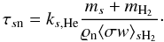 (A.1)The quantity ks,He is a correction factor entering the equation due to the fact that the gas also contains helium. The above expression hence calculates the collision time for a charged species s with all neutrals. Helium contributes only a small correction factor due to its low polarizability compared with H2 (Spitzer 1978). Mouschovias (1996) gives these correction factors as
 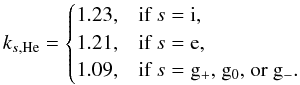 (A.2)The values for the rate constant ⟨ σw ⟩ sH2 are taken from McDaniel & Mason (1973), Mott & Massey (1965), and Ciolek & Mouschovias (1993), respectively:
 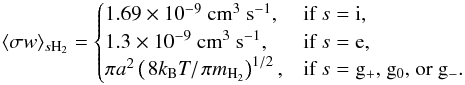 (A.3)The last expression assumes that the difference between the grain and neutral velocities is smaller than the sound speed.
Appendix B: Rate coefficients
For convenience, we reproduce here the rate coefficients used in this work. They can also be found in Appendix A of Kunz & Mouschovias (2009).
For radiative recombination of atomic ions and electrons, and for the dissociative recombination of electrons and HCO + ions, we respectively adopt the values (Umebayashi & Nakano 1990) 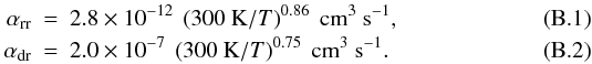 For charge-exchange reactions between atomic and molecular ions, we use the value from Watson (1976):
 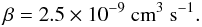 (B.3)The rate coefficients pertaining to ions (both molecular and atomic, indicated with subscript “i”) and electrons (subscript “e”) on the one hand and grains on the other are taken from Spitzer (1941, 1948), with refinements made by Draine & Sutin (1987) to account for the polarization of grains:
 ![Mathematical equation: \appendix \setcounter{section}{2} \begin{eqnarray} \alpha_{\mathrm{e}\mathrm{g}^{0}} &=& \pi a^{2} \left(\frac{8k_\mathrm{B}T}{\pi m_{\mathrm{e}}} \right)^{1/2} \left[1+ \left(\frac{\pi e^{2}}{2ak_\mathrm{B}T}\right)^{1/2} \right] \mathcal{P}_{\mathrm{e}}, \\ \alpha_{\mathrm{i}\mathrm{g}^{0}} &=& \pi a^{2} \left(\frac{8k_\mathrm{B}T}{\pi m_{\mathrm{i}}} \right)^{1/2} \left[1+ \left(\frac{\pi e^{2}}{2ak_\mathrm{B}T}\right)^{1/2} \right] \mathcal{P}_{\mathrm{i}}, \\ \alpha_{\mathrm{e}\mathrm{g}^{+}} &=& \pi a^{2} \left(\frac{8k_\mathrm{B}T}{\pi m_{\mathrm{e}}} \right)^{1/2} \left[1+ \left(\frac{e^{2}}{ak_\mathrm{B}T}\right) \right] \notag \\ &&\qquad \times \left[1+ \left(\frac{2 e^{2}}{2e^{2}+ak_\mathrm{B}T}\right)^{1/2} \right] \mathcal{P}_{\mathrm{e}}, \\ \alpha_{\mathrm{i}\mathrm{g}^{-}} &=& \pi a^{2} \left(\frac{8k_\mathrm{B}T}{\pi m_{\mathrm{i}}} \right)^{1/2} \left[1+ \left(\frac{e^{2}}{ak_\mathrm{B}T}\right) \right] \notag \\ \label{eq:alpha_ei_g} &&\qquad \times \left[1+ \left(\frac{2 e^{2}}{2e^{2}+ak_\mathrm{B}T}\right)^{1/2} \right] \mathcal{P}_{\mathrm{i}}. \end{eqnarray}](/articles/aa/full_html/2012/05/aa17876-11/aa17876-11-eq396.png) For the sticking probabilities of electrons or ions onto grains, we take the values from Umebayashi (1983),
For the sticking probabilities of electrons or ions onto grains, we take the values from Umebayashi (1983),  and
and  . In these equations, a is the adopted grain radius, while other quantities have their usual meanings. Lastly, the rate coefficients for charge transfer during collisions between grains are of the same form as the ones above, but with modified masses:
 ![Mathematical equation: \appendix \setcounter{section}{2} \begin{eqnarray} \alpha_{\mathrm{g}^{+}\mathrm{g}^{-}} &=& 16\pi a^{2} \left(\frac{k_\mathrm{B}T}{\pi m_{\mathrm{g}}} \right)^{1/2} \left[1+ \left(\frac{e^{2}}{2ak_\mathrm{B}T}\right) \right] \notag \\ \label{eq:alpha_gg} &&\qquad\qquad \times \left[1+ \left(\frac{e^{2}}{e^{2}+ak_\mathrm{B}T}\right)^{1/2} \right],\\ \label{eq:alpha_gg0} \alpha_{\mathrm{g}^{\pm}\mathrm{g}^{0}} &=& 16\pi a^{2} \left(\frac{k_\mathrm{B}T}{\pi m_{\mathrm{g}}} \right)^{1/2} \left[1+ \left(\frac{\pi e^{2}}{4ak_\mathrm{B}T}\right)^{1/2} \right] \mathcal{P}_{\mathrm{gg}}. \end{eqnarray}](/articles/aa/full_html/2012/05/aa17876-11/aa17876-11-eq399.png) Here, mg is the grain mass (assumed constant), and
Here, mg is the grain mass (assumed constant), and  is the probability of charge exchange between neutral and charged grains (both positive and negative). The probability of neutralization in Eq. (B.8) is assumed to be unity.
All Tables
All Figures
|
Fig. 1 Column number density profile versus radius for Model 2. The thin lines (in ascending order) are plots at the times listed in Table 2. Several features are identifiable via their associated breaks in the profile. (1) Prestellar infall profile with N ∝ r-1. (2) Magnetic wall at ≈10 AU, where the bunched-up field lines decelerate material before it continues the infall. (3) Expansion wave profile with N ∝ r−1/2 outside the first core. (4) First core at 1 AU. (5) Infall profile onto the second core with N ∝ r-1. After the first core has reached ≈1000 K, it starts to collapse, as H2 is dissociated. (6) Expansion wave profile with N ∝ r−1/2 outside the second core. (7) Second core at ≈1 R⊙. |
| In the text | |
|
Fig. 2 Central diffusion coefficient ηeff versus number density for different grain sizes, extracted from the dynamical model. The vertical line at the left indicates the density at which the detailed chemistry and non-ideal MHD treatment is switched on. Beyond nc ≈ 1018 cm-3 the resistivity plummets, after having already declined due to thermal ionization. This is where we switch the chemistry calculations off again, and is denoted by the vertical line on the right. Due to grain destruction, flux-freezing is restored there. |
| In the text | |
|
Fig. 3 Diffusion coefficient versus grain size for two values of number density. The diffusion coefficient behaves qualitatively differently at different densities. While at high densities, the diffusion coefficient increases monotonically with increasing grain radius, it has a maximum for low densities at a grain size of agr ≈ 0.065 μm. Below this radius, the effect of better coupling dominates, while at larger grain sizes the decreased surface area of the larger grains leaves more free gas-phase charges, with associated higher conductivity, and conversely decreased resistivity. |
| In the text | |
|
Fig. 4 Contributions due to ambipolar diffusion (AD) and Ohmic dissipation (OD) to the effective resistivity in Model 2 (grain size agr = 0.038 μm) at the end of the run. OD only dominates AD beyond nc ≈ 1012 cm-3, within the first core. |
| In the text | |
|
Fig. 5 Total ionization fraction versus central density for different grain sizes. The vertical line indicates the density at which the detailed chemistry and non-ideal MHD treatment is switched on. |
| In the text | |
|
Fig. 6 Central fractional abundances of species. Top left: Model 1, agr = 0.019 μm, middle left: Model 2, agr = 0.038 μm, bottom left: Model 3, agr = 0.075 μm. The convergence of the abundances of positively- and negatively-charged grains is pushed to higher densities with increasing grain radius. The departure of the electron abundance from the ion abundance also happens at higher densities with decreasing grain surface area. The dashed vertical line at nc ≈ 106 cm-3 indicates the density at which the chemistry and non-ideal MHD treatment are switched on, while the one at nc ≈ 3 × 1018 cm-3 shows when we assume the destruction of grains restores flux-freezing. Top right: Model 4, agr = 0.113 μm, bottom right: Model 5, agr = 0.150 μm. Since the grain radius increases only by a factor of 4/3 from Model 4, the effect on the abundances is less pronounced than it was for the smaller grains. |
| In the text | |
|
Fig. 7 Mass-to-flux ratio μ versus radius for different grain sizes at the time of the formation of the second core. For comparison, the thin dashed line shows the case with only the simplified version of Ohmic dissipation, as used in DB10. In the center, the difference is a factor of ≈ 102, but further out it it still 2 × higher, and also shows a greater extent by about this factor. The reason is twofold: firstly, ambipolar diffusion is important at lower densities and, secondly, the effective resistivity is larger everywhere than the parametrization used in DB10 (cf. Fig. 2). |
| In the text | |
|
Fig. 8 Evolution of Bz versus radius over time. The thin lines are plots at the times listed in Table 2, for the fiducial grain radius of agr = 0.038 μm. |
| In the text | |
|
Fig. 9 Evolution of the angular velocity Ω versus radius over time. The thin lines are plots at the times listed in Table 2, for the fiducial grain radius of agr = 0.038 μm. The profile changes from being ∝ r-1 to ∝ r-2 in the expansion wave, as expected from theoretical considerations. |
| In the text | |
|
Fig. 10 Evolution of the infall radial velocity |vr| versus radius over time. The thin lines are plots at the times listed in Table 2, for the fiducial grain radius of agr = 0.038 μm. Outside the first core, the magnetic wall causes a small bump. Within the first and second cores material is moving about inwards and outwards with small speeds. This causes spikes when absolute values are plotted on double-logarithmic axes. |
| In the text | |
|
Fig. 11 Evidence for disk formation. Top panel: column density profile. The system is Toomre-unstable, and breaks up into a ring in the resistive model (solid line), but not in the flux-frozen model (dotted line). Middle panel: infall profile. Infall is stopped in the resistive model (solid line), in innermost region where a centrifugal disk forms, but not in the flux-frozen model (dotted line). Bottom panel: ratio of centrifugal over gravitational acceleration. In the resistive model, centrifugal balance is achieved. In contrast, catastrophic magnetic braking occurs for the flux-frozen model, the centrifugal support drops to negligible values and the first core is spun down drastically. |
| In the text | |
|
Fig. 12 Magnetic field lines. The box on the left has dimensions 10 AU on each side, while the box on the right has dimensions 100 AU. The dashed lines represent the flux-freezing model, while the solid lines show the same field lines for the model including non-ideal MHD effects for a grain size agr = 0.038 μm. In both cases, the second core has just formed and is on the left axis midplane. The field lines straighten out significantly on small scales in the non-ideal model compared to the flux-frozen model. |
| In the text | |
|
Fig. 13 Plot of the ratio τMB/τdyn. For both the flux-freezing case (dashed line) as well for non-ideal MHD (solid line), the magnetic braking time is reduced in the expansion wave region from what is was in the prestellar infall region. In the case of non-ideal MHD, it turns up sharply at the interface of the first core where diffusion has reduced the magnetic field strength significantly and rendered magnetic braking ineffective. In the flux frozen case however, the first core marks a sharp drop in magnetic braking time to only a tenth of the dynamical time. |
| In the text | |
|
Fig. 14 Estimated centrifugal radius of each mass shell. Beyond ≈ 10 AU, the centrifugal radius increases linearly. The solid line is the current centrifugal radius, while the dotted line is an estimate of rcf after the expansion wave has passed and the associated magnetic braking has reduced the specific angular momentum (see text). The top axis shows the approximate times at which the expansion wave is expected to pass a certain radius. The symbols show the estimated centrifugal radii of 1 AU and 10 AU. The associated times are 6 × 10³ yr and 4 × 10⁴ yr. |
| In the text | |
|
Fig. 15 Ratio of Br/Bz,eq. In the flux frozen case (dashed line), Br dominates everywhere within the expansion wave, indicative of extreme flaring and a split-monopole field configuration. With field diffusion active (solid line), the field lines straighten out quickly inside the expansion wave (cf. Fig. 12). |
| In the text | |
|
Fig. 16 Ratio of diffusion time τdiff and dynamical time τdyn at the end of the run. Within the expansion wave, the ratio is smaller than unity, and diffusion dominates over advection. |
| In the text | |
|
Fig. 17 Specific angular momentum versus enclosed mass at initial state (dashed line) and final snapshot (solid line), and their ratio (dotted line). The expansion wave brings with it a maximal reduction of specific angular momentum. Further insight is provided by the radius versus enclosed mass, plotted as the dot-dashed line, with radius values denoted on the second axis on the right. |
| In the text | |
Current usage metrics show cumulative count of Article Views (full-text article views including HTML views, PDF and ePub downloads, according to the available data) and Abstracts Views on Vision4Press platform.
Data correspond to usage on the plateform after 2015. The current usage metrics is available 48-96 hours after online publication and is updated daily on week days.
Initial download of the metrics may take a while.