| Issue |
A&A
Volume 540, April 2012
|
|
|---|---|---|
| Article Number | L13 | |
| Number of page(s) | 4 | |
| Section | Letters | |
| DOI | https://doi.org/10.1051/0004-6361/201118657 | |
| Published online | 06 April 2012 | |
Outflow and accretion detections in the young stellar object IRAS 04579+4703
1 National Astronomical Observatories, Chinese Academy of Sciences, Beijing 100012, PR China
e-mail: This email address is being protected from spambots. You need JavaScript enabled to view it.
2 Graduate University of the Chinese Academy of Sciences, 100080 Beijing, PR China
3 I. Physikalisches Institut, Universität zu Köln, Zülpicher Str. 77, 50937 Köln, Germany
Received: 16 December 2011
Accepted: 16 March 2012
Abstract
We present Submillimeter Array observations of the young stellar object IRAS 04579+4703 in the 1.3 mm continuum and in the 12CO(2−1), 13CO(2−1), and C18O(2−1) lines. The 1.3 mm continuum image reveals a flattened structure with a mass of 13 M⊙. The 12CO(2−1) line map and position-velocity diagram, together with the broad wing (full width = 30 km s-1) of the 12CO(2−1) line, clearly show that there is an outflow motion, which originates from an embedded massive YSO in this region. The lengths of the blue-shifted and red-shifted lobes are 0.14 pc and 0.13 pc, respectively. The total gas mass, average dynamical timescale, and mass entrainment rate of the outflow are 1.8 M⊙, 1.7 × 10⁴ yr and 1.1 × 10⁻⁴M⊙ yr-1, respectively. The flattened morphology of the continuum source perpendicular to the outflow direction, and the velocity gradient seen in the spectra of C18O(2−1) taken from different locations along the major axis of the continuum source, suggest that there is an accretion disk in this region.
Key words: ISM: individual objects: IRAS 04579+4703 / ISM: kinematics and dynamics / ISM: molecules / stars: formation
© ESO, 2012
1. Introduction
Observational evidence suggests that massive stars may be formed by means of accretion-disk-outflow processes similar to those operating in low-mass stars (e.g, Shu et al. 1987; Cesaroni et al. 1999; Shepherd et al. 2001; Patel et al. 2005; Jiang et al. 2005; Zinnecker & Yorke 2007). This has been a rapid increase in the number of searches for collapse, accretion, and outflow with interferometers in massive star-formation regions (e.g, Beuther et al. 2004; Qin et al. 2008; Furuya et al. 2011), but the still limited available observations cannot provide the detailed information required to improve our understanding of massive star formation. The major difficulty is due to the large distances of the typical targets (≥1 kpc), the clustered formation environments, and the shorter evolutionary timescales of massive stars.
IRAS 04579+4703 is a young high-mass stellar object (YSO). Molinari et al. (1996) carried out the NH3 observation toward IRAS 04579+4703, and obtained a distance of 2.47 kpc from the Sun and a bolometric luminosity of 3.91 × 10³ L⊙. However, Molinari et al. (1998a) failed to observe any 6 cm emission from IRAS 04579+4703. Sánchez-Monge et al. (2008) performed higher spatial resolution continuum observations at 1.2 mm, 7 mm, 1.3 cm, and 3.6 cm toward IRAS 04579+4703. Their observations showed that the 7 mm emission, which is similar to the 1.3 cm and 3.6 cm emission in terms of morphology, is elongated in the southwest-northeast direction. The location of their 1.2 mm continuum peak agrees well with that of the source detected at cm wavelengths as well as an H2O maser (Palla et al. 1991; Migenes et al. 1999), indicating that the emissions only concentrate on a small and compact region and that IRAS 04579+4703 is at an early evolutionary stage. Using the SED fit, Sánchez-Monge et al. (2008) derived a dust temperature of about 30 K and inferred a gas mass of 23 M⊙. The 12CO(2−1) line observations of Zhang et al. (2005) did not reveal molecular outflow from IRAS 04579+4703, while Wouterloot & Brand (1989) observed the 12CO(1−0) emission with a linewidth of 6.1 km s-1. Additionally, Varricatt et al. (2010) detected jet-like H2 knots in the northwest-southeast direction. However, these observations cannot provide sufficient evidence of the outflow. Higher spatial resolution observations of the molecular lines and continuum in submillimeter/millimeter waveband are needed to reveal the detailed source structure and kinematics in this region.
In this Letter, we present Submillimeter Array (SMA) observations of the young stellar object IRAS 04579+4703 obtained in the 1.3 mm continuum and in the 12CO(2−1), 13CO(2−1), and C18O(2−1). Our observations at high angular resolution reveal bipolar outflow motion and gas accretion for IRAS 04579+4703.
2. Observations and data reduction
The observations toward IRAS 04579+4703 were performed with the SMA on 2008 March 21, at 220 GHz (lower sideband) and 230 GHz (upper sideband)1. The two sidebands of the SMA covered frequency ranges of 219.4–221.4 GHz and 229.4–231.4 GHz, respectively. The projected baselines ranged from 7 kλ to 100 kλ. The phase track center was RA(J2000.0 and Dec(J2000.0) =
  . The typical system temperature was 186 K. The spectral resolution is 0.406 MHz, corresponding to a velocity resolution of 0.5 km s-1. The bright quasar 3C 279 was used for bandpass calibration, while absolute flux density scales were determined from observations of Titan. QSO 0533+483 and QSO 0359+509 were observed for antenna gain corrections. The calibration and imaging were performed in Miriad. A continuum image was constructed from the line-free channels. The spectral cubes were constructed using the continuum-subtracted spectral channels. Self-calibration was performed on the continuum data. The gain solutions from the continuum were applied to the line data. The synthesized beam size of the continuum was approximately
  ×
×  with a
  . On the basis of the phase monitoring of QSO 0533+483, the absolution position accuracy (pointing error) is estimated to be ~0.1′′ during the observations.
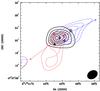 |
Fig. 1 The 1.3 mm continuum emission (black thicker contours) overlaid with the velocity-integrated intensity map of 12CO(2−1) outflow (red and blue contours). The black contour levels are at 3, 6, 9, 12, 15, 18, and 21σ (1σ is 0.002 Jy beam-1). The red and blue contour levels are 35, 50,..., 95% of the peak value. The synthesized beam is |

3. Results
3.1. Continuum emission at 1.3 mm
In Fig. 1, the 1.3 mm continuum image observed with the SMA shows a flattened source structure. Using a two-dimensional Gaussian fit to the continuum, we obtained a total integrated flux density of 0.11 Jy, a deconvolved source size of 4.7′′ × 2.9′′ (PA = 83.1°), and a peak position of RA(J2000) = 05h01m40 086, Dec(J2000) = +47°07′20
 90. The positional uncertainty caused by noise can be estimated to be △ θ = 0.45
  , where θFWHM is the angular resolution and S/N is the signal-to-noise ratio (Reid et al. 1988; Chen et al. 2006; Weintroub et al. 2008; Qin et al. 2010). The estimated positional uncertainty is approximately
  . If we also consider the uncertainty in both establishing with a Gaussian fit the position of the continuum peak and the pointing error, then ΔRA = ± 0.24′′ and ΔDec = ± 0.21′′. The 1.3 mm continuum emission is associated with an H2O maser (Migenes et al. 1999), as well as a near-IR source detected by Varricatt et al. (2010). In addition, the peak of the 1.3 mm continuum agrees well with those of the 1.3 cm, 3.6 cm, and 7 mm emission within the positional uncertainty (Sánchez-Monge et al. 2008). Sánchez-Monge et al. (2008) argued that these radio emission could originate from either radio jets or hypercompart HII regions. The increasing spectral index with frequence (Sánchez-Monge et al. 2008), association with an H2O maser, and compact source structure suggest that there is a hypercompact HII region in this region (Sewilo et al. 2004). Therefore the 1.3 mm continuum emission may comprise free-free emission from the hypercompart HII region and the thermal emission from the warm dust from its surroundings (Keto et al. 1988; Beltrán et al. 2011). The emission from the free-free component of the continuum flux in our source can be estimated by Sν ∝ να, where the free-free spectral index α is 1.1 from 3.6 cm to 1.3 cm continuum emission. The contribution of the free-free emission to the 1.3 mm continuum is ~ 4.4 mJy (much lower than our total integrated flux 0.11 Jy at 1.3 mm), and can then safely be ignored.
To determine the total gas mass of the continuum source, we make the optically thin approximation for the dust continuum emission. The total gas mass of the continuum source can be estimated by Mcore = SvD2/κνRBν(Td), where Sv is the flux at the frequency ν and D is the distance to the source. We assume κν = 0.05(ν/230)β m2 kg-1 for the opacity (Testi & Sargent 1998), where we adopt β = 2 (Drain & Lee 1984) and a dust-to-gas mass ratio R = 0.01 (Lis et al. 1991), and Bv(Td) is the Planck function for a dust temperature Td at frequency ν. Using a dust temperature of ~ 30 K (Sánchez-Monge et al. 2008), we derive a total gas mass of 13 M⊙. Because the extended envelope can be filtered by the interferometers, which are missing short spacing data, the mass of the gas derived from our data is lower than 23 M⊙ according to the single dish observations (Sánchez-Monge et al. 2008).
Physical parameters of the outflow.
3.2. Molecular line emission
Figure 2 shows the spectra of 12CO(2−1), 13CO(2−1), and C18O(2−1) emission at the peak position of the continuum image. The 12CO(2−1) and 13CO(2−1) lines clearly display asymmetric profiles with double peaks, which may be caused by large optical depths (André et al. 1999; Belloche et al. 2002). The C18O(2−1) line with a single emission peak can be considered as optically thin, hence can be used to determine the systemic velocity. We measure a systemic velocity of ~−17.0 km s-1 for this line. The velocities of the blue and red emission peaks of 12CO(2−1) are −20 km s-1 and − 13 km s-1. For 13CO(2−1), the velocities of the blue and red emission peaks are − 19 km s-1 and −16 km s-1.
The 12CO(2−1) and 13CO(2−1) spectra show a “blue profile” signature (Wu et al. 2007), and the blue peaks of both lines are stronger than their red peaks with an absorption dip near the systemic velocity, which may be produced by infall motion or accretion. In addition, the 12CO(2−1) spectrum has an unusual full width of ~30 km s-1, from − 38 to −8 km s-1. Such a broad wing is a strong indication of outflow motion.
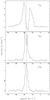 |
Fig. 2 Spectral profiles observed at the central position of IRAS 04579+4703 in the optically thick 12CO(2−1), 13CO(2−1) lines, and the optically thin C18O(2−1) line. The dotted line in the spectra marks the cloud systemic velocity. |
To determine the velocity components and spatial extension of the outflow, we compiled a position-velocity (PV) diagram along the cuts at various position angles, and found that the redshifted and blueshifted components are the strongest at a position angle of −40° (40° west of north) as shown in Fig. 3. The PV diagram in Fig. 3 clearly shows bipolar components. The blueshifted and redshifted components have obvious velocity gradients from −24.2 to −20 km s-1 and −13 to −8.5 km s-1, respectively (see the blue and red vertical dashed lines in Fig. 3). The distributions of redshifted and blueshifted velocity components in Fig. 3 provide further evidence of a bipolar outflow in this region (Yamashita et al. 1989).
Using the velocity ranges determined from the PV diagram, we made velocity-integrated intensity maps superimposed on the 1.3 mm continuum as shown in Fig. 1. The blueshifted and redshifted components are presented as blue and red contours. The map clearly displays northwest-southeast bipolar components centered at the peak position of the 1.3 mm continuum. The blueshifted and redshifted lobes are not in a straight line. The outflow is associated with an infrared source IRAS 04579+4703 and a near-IR source.
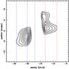 |
Fig. 3 The position-velocity plot of the 12CO(2−1) emission at a position angle of −40°. The contour levels are 1.4, 1.8, 2.3, 2.7, 3.2, 3.6, 4.1, and 4.5 Jy beam-1, and 1 σ is 0.7 Jy beam-1. The black vertical dashed line marks the cloud systemic velocity. The blue and red vertical dashed lines mark the velocity ranges of the blueshifted and redshifted emission, respectively. |
4. Discussion
4.1. Outflow kinematics and driving source
The velocity-integrated intensity map, PV diagram, and the broad wing (full width = 30 km s-1) of the CO 12CO(2−1) line clearly show evidence of a bipolar outflow in IRAS 04579+4703 region. The blueshifted and redshifted lobes do not lie on a straight line, and the extension is similar to that of H2 knots (Varricatt et al. 2010), indicating that the H2 and CO data most likely represent the same outflow, and that the 12CO(2−1) outflow gas is probably entrained by the H2 jet-like outflow. The outflow is associated with the infrared source IRAS 04579+4703 and a near-IR source. Varricatt et al. (2010) suggested that the near-IR source may be the near-IR counterpart of IRAS 04579+4703 with the strong infrared excess. The position of the near-IR source agrees well with the peaks of the 1.3 mm, 7 mm, 1.3 cm and 3.6 cm emission within the positional uncertainty. Both H2 and Brγ emission are very close to the near-IR source (Ishii et al. 2001; Varricatt et al. 2010). Interpreting the data together, we conclude that the near-IR source may be an embedded massive YSO, which is likely to drive the bipolar outflow.
Under conditions of local thermodynamical equilibrium (LTE), since 12CO(2−1) is optically thick, and the beam is completely filled by the source (the filling factor f = 1), the column density of the outflow is estimated following Garden et al. (1991) with a relation NH2 ≈ 104N12CO (Dickman 1978) using the equation: ![Mathematical equation: \begin{equation} \mathit{N_{\rm H_{2}}}\!=\!1.08\!\times\!10^{17}\frac{(T_{\rm ex}+0.92)}{\exp(-16.62/T_{\rm ex})}\!\!\int\!\! T_{\rm mb}\!\times\!\frac{\tau {\rm d}v}{[1-\exp(-\tau)]}~{\rm cm}^{-2}, \end{equation}](/articles/aa/full_html/2012/04/aa18657-11/aa18657-11-eq81.png) (1)where Tex is the excitation temperature, Tmb is the corrected main-beam temperature, and τ is the optical depth of the 12CO(2−1) line. We assume the solar abundance ratio [12CO]/[C18O] = τ(12CO)/τ(C18O) = 490 (Garden et al. 1991), and estimate Tex following the equation Tex = 11.1/ln [1 + 1/(Tmb/11.1 + 0.02)] (Garden et al. 1991). The red-lobe and blue-lobe peaks of the outflow near the continuum, then we assume that the 12CO and C18O trace the same cloud components at the peak positions of the two lobes for in calculation, and the assumption is reasonable since both 12CO(2−1) and C18O(2−1) are low energy transition with similar upper level energy. Under the assumption that C18O is optically thin, we calculate τ according to
(1)where Tex is the excitation temperature, Tmb is the corrected main-beam temperature, and τ is the optical depth of the 12CO(2−1) line. We assume the solar abundance ratio [12CO]/[C18O] = τ(12CO)/τ(C18O) = 490 (Garden et al. 1991), and estimate Tex following the equation Tex = 11.1/ln [1 + 1/(Tmb/11.1 + 0.02)] (Garden et al. 1991). The red-lobe and blue-lobe peaks of the outflow near the continuum, then we assume that the 12CO and C18O trace the same cloud components at the peak positions of the two lobes for in calculation, and the assumption is reasonable since both 12CO(2−1) and C18O(2−1) are low energy transition with similar upper level energy. Under the assumption that C18O is optically thin, we calculate τ according to ![Mathematical equation: \hbox{$\tau=\rm-490\,ln[1-(e^{11.1/\it T_{\rm ex}}-1) T^{18}_{\rm mb}/\rm 11.1]$}](/articles/aa/full_html/2012/04/aa18657-11/aa18657-11-eq89.png) (Garden et al. 1991). Under the Rayleigh-Jeans approximation, 1 Jy beam-1 in our SMA observations corresponds to a brightness temperature of 2.52 K. Furthermore, the mass of the outflow is given by Mout = mNH2S/(2.0 × 1033) M⊙, where m is 1.36 times the H2 mass (Garden et al. 1991) and S is the size of each lobe and obtained from the deconvolved lobe size (in Table 1). A dynamic timescale can be determined by td = r/v, where v is the maximum flow velocity relative to the cloud systemic velocity, and r is the length of the begin-to-end flow extension for each lobe. The lengths of the blueshifted and redshifted lobes obtained from Fig. 1 are 0.14 pc and 0.13 pc, respectively, which is only a lower limit owing to projection onto the sky plane. The mass entrainment rate of the outflow is calculated using Ṁout = Mout/(td). The physical parameters and the calculated results of the outflow are summarized in Table 1. The difference in the parameters of the two lobes reflects that the lack of uniformity of the ambient material, hence the different masses and dynamics. The outflow has a total mass of 1.8 M⊙ and a mass entrainment rate of 1.1 × 10⁻⁴M⊙ yr-1. The average dynamical timescale is about 1.7 × 10⁴ yr.
(Garden et al. 1991). Under the Rayleigh-Jeans approximation, 1 Jy beam-1 in our SMA observations corresponds to a brightness temperature of 2.52 K. Furthermore, the mass of the outflow is given by Mout = mNH2S/(2.0 × 1033) M⊙, where m is 1.36 times the H2 mass (Garden et al. 1991) and S is the size of each lobe and obtained from the deconvolved lobe size (in Table 1). A dynamic timescale can be determined by td = r/v, where v is the maximum flow velocity relative to the cloud systemic velocity, and r is the length of the begin-to-end flow extension for each lobe. The lengths of the blueshifted and redshifted lobes obtained from Fig. 1 are 0.14 pc and 0.13 pc, respectively, which is only a lower limit owing to projection onto the sky plane. The mass entrainment rate of the outflow is calculated using Ṁout = Mout/(td). The physical parameters and the calculated results of the outflow are summarized in Table 1. The difference in the parameters of the two lobes reflects that the lack of uniformity of the ambient material, hence the different masses and dynamics. The outflow has a total mass of 1.8 M⊙ and a mass entrainment rate of 1.1 × 10⁻⁴M⊙ yr-1. The average dynamical timescale is about 1.7 × 10⁴ yr.
4.2. Accretion
Our interferometric continuum image toward IRAS 04579+4703 reveals a flattened structure, perpendicular to the direction of the outflow detected in 12CO(2−1) and H2, which is consistent with the accretion disk scenario proposed for the other high-mass star-formation regions (Cesaroni et al. 1999; Shepherd et al. 2001; Patel et al. 2005). The C18O(2−1) spectra from the two positions (the red and blue plus symbols in Fig. 1) perpendicular to the direction of the outflow are shown in Fig. 4. The velocity gradient is seen from the C18O(2−1) spectra, suggesting that the disk is rotationally and gravitationally bound by the central YSO. Assuming that the rotation is Keplerian, the dynamical mass (binding mass) is estimated to be M = δv2r/G sin2(i), where r is the half spatial separation of the emission, δv is the difference between the peak velocity of the emission and the systemic velocity, and i is the unknown inclination angle between the disk plane and the plane of the sky (i = 90° for an edge-on system). Adopting the values r ~ 2′′ and δv ~ 1 km s-1 shown in Figs. 1 and 4, the obtained dynamical mass is ~6/[sin2(i)] M⊙. The dynamical mass is estimated to be 12 M⊙ if i = 45°, which is a lower limit since we estimated the binding mass from the kinematics inside 2′′ owing to our low spatial resolution observations.
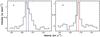 |
Fig. 4 C18O(2−1) spectra. In the a) and b) panels, the molecular spectra are extracted from the positions of the blue and red plus symbols marked in Fig. 1, respectively, which are separated by 4′′. The black vertical dashed line marks the cloud systemic velocity. The blue and red vertical dashed lines mark the peak velocities, respectively. |
The spectroscopic observations of H2 and Brγ (Ishii et al. 2001) implied that the source contains an accretion disk that is probably accreting. If we assume that the central star is a massive protostar and not a zero-age main-sequence (ZAMS) star, then its bolometric luminosity (3.91 × 10³ L⊙) is equal to the accretion luminosity. According to Molinari et al. (1998b), the accretion rate is given by Ṁ = 6.22 × 10⁻⁹(L/L⊙)1.70(M/M⊙)-1.24. Assuming that the dynamical mass of 12 M⊙ is equal to the protostar mass, the expected accretion rate is 3.7 × 10⁻⁴ M⊙yr-1.
The “blue profile” of the 12CO(2−1) line provide further evidence for the infall motion or accretion discussed in Sect. 3.2. The mass accretion rate is estimated to be Ṁ = 4πR2Vmn (Myers et al. 1996), where m is 1.36 times the H2 mass. If the cloud core is approximately spherical in shape, its mean number density is n = 1.62 × 10⁻¹⁹NH2/L, where L is the cloud core diameter in parsecs, which is 0.056 pc (the major axis of the deconvolved size of the continuum) and N(H2) is the column density of molecular hydrogen obtained from Eq. (3) of Xu et al. (2010) for the C18O line. The velocity difference (V) of 2.0 km s-1 between the systemic velocity (–17.0 km s-1) and the velocity of the redshifted absorbing dip (–15.0 km s-1) and a source size (R) of 0.028 pc, then implies a mass accretion rate of ~2.3 × 10⁻⁴ M⊙ yr-1, which is roughly consistent with the value derived from bolometric luminosity, providing additional evidence of an accretion disk in this region, although observations at the presently achievable spatial resolution are inadequate to distinguish the disk accretion and the observations of other molecular tracers at higher spatial resolution are needed to resolve the detailed kinematics in this region.
The data are publicly available at the website http://www.cfa.harvard.edu/rtdc/data/search.html
Acknowledgments
We thank the anonymous referee for his/her constructive comments and suggestions that greatly improved the content and presentation of this paper. Jin-Long Xu’s research is in part supported by 2011 Ministry of Education doctoral academic prize.
References
- André, P., Motte, F., & Bacmann, A. 1999, ApJ, 513, L57 [NASA ADS] [CrossRef] [Google Scholar]
- Belloche, A., André, P., Despois, D., & Blinder, S. 2002, A&A, 393, 927 [Google Scholar]
- Beltrán, M. T., Cesaroni, R., Neri, R., & Codella, C. 2011, A&A, 525, A151 [NASA ADS] [CrossRef] [EDP Sciences] [Google Scholar]
- Beuther, H., Hunter, T. R., & Zhang, Q. 2004, ApJ, 616, 23 [Google Scholar]
- Cesaroni, R., Felli, M., Jenness, T., et al. 1999, A&A, 345, 949 [NASA ADS] [Google Scholar]
- Chen, H.-R., Welch, W. J., Wilner, D. J., & Sutton, E. C. 2006, ApJ, 639, 975 [NASA ADS] [CrossRef] [Google Scholar]
- Dickman, R. L. 1978, ApJ, 37, 407 [Google Scholar]
- Draine, B. T., & Lee, H. M. 1984, ApJ, 285, 89 [Google Scholar]
- Furuya, R. S., Cesaroni, R., & Shinnaga, H. 2011, A&A, 525, A72 [NASA ADS] [CrossRef] [EDP Sciences] [Google Scholar]
- Garden, P. R., Hayashi, M., Hasegawa, T., et al. 1991, ApJ, 374, 540 [NASA ADS] [CrossRef] [Google Scholar]
- Ishii, M., Nagata, T., Sato, S., et al. 2001, AJ, 121, 3191 [NASA ADS] [CrossRef] [Google Scholar]
- Jiang, Z., Tamura, M., Fukagawa, M., et al. 2005, Nature, 437, 112 [NASA ADS] [CrossRef] [PubMed] [Google Scholar]
- Keto, E. R., Ho, P. T. P., & Haschick, A. D. 1988, ApJ, 324, 920 [NASA ADS] [CrossRef] [Google Scholar]
- Lang, K. R. 1980 Aatrophysical Formulae (Berlin: Springer-Verlag) [Google Scholar]
- Lis, D. C., Carlstrom, J. E., & Keene, J. 1991 ApJ, 380, 429 [Google Scholar]
- Migenes, V., Horiuchi, S., Slysh, V. I., et al. 1999, ApJS, 123, 487 [NASA ADS] [CrossRef] [Google Scholar]
- Molinari, S., Brand, J., Cesaroni, R., & Palla, F. 1996, A&A, 308, 573 [NASA ADS] [Google Scholar]
- Molinari, S., Brand, J., Cesaroni, R., et al. 1998a, A&A, 336, 339 [NASA ADS] [Google Scholar]
- Molinari, S., Testi, L., Brand, J., et al., 1998b, ApJ, 505, L39 [NASA ADS] [CrossRef] [Google Scholar]
- Myers, P. C., Mardones, D., Tafalla, M., et al. 1996, ApJ, 465, L133 [NASA ADS] [CrossRef] [Google Scholar]
- Palla, F., Brand, J., Comoretto, G., et al. 1991, A&A, 246, 249 [NASA ADS] [Google Scholar]
- Patel, N. A., Curiel, S., Sridharan, T. K., et al. 2005, Nature, 437, 109 [NASA ADS] [CrossRef] [PubMed] [Google Scholar]
- Qin, S.-L., Zhao, J.-H., & Moran, J. M. 2008, ApJ, 677, 353 [NASA ADS] [CrossRef] [Google Scholar]
- Qin, S.-L., Wu, Y. F., Huang, M. H., et al. 2010, ApJ, 711, 399 [NASA ADS] [CrossRef] [PubMed] [Google Scholar]
- Reid, M. J., Schneps, M. H., Moran, J. M., et al. 1988, ApJ, 330, 809 [NASA ADS] [CrossRef] [Google Scholar]
- Sánchez-Monge, Á., Aina, P., Estalella, R., Beltrán, M. T., & Girart, J. M. 2008, A&A, 485, 497 [NASA ADS] [CrossRef] [EDP Sciences] [Google Scholar]
- Sewilo, M., Churchwell, E., Kurtz, S., et al., 2004, ApJ, 605, 285 [NASA ADS] [CrossRef] [Google Scholar]
- Shepherd, D., Claussen, M. J., & Kurtz, S. E. 2001, Science, 292, 1513 [NASA ADS] [CrossRef] [PubMed] [Google Scholar]
- Shu, F. H., Adams, F.C., & Lizano, S. 1987, ARA&A, 25, 23 [Google Scholar]
- Testi, L., & Sargent, A. I. 1998, ApJ, 508, L91 [NASA ADS] [CrossRef] [Google Scholar]
- Varricatt, W. P., Davis, C. J., Ramsay, S., & Todd, S. P. 2010, MNRAS, 404, 661 [NASA ADS] [CrossRef] [Google Scholar]
- Weintroub, J., Moran, J. M., Wilner, D. J., et al. 2008, ApJ, 677, 1140 [NASA ADS] [CrossRef] [Google Scholar]
- Wouterloot, J. G. A., & Brand, J. 1989, A&AS, 80, 149 [NASA ADS] [Google Scholar]
- Wu, Y., Henkel, C., Xue, R., Guan, X., & Miller, M. 2007, ApJ, 669, L37 [NASA ADS] [CrossRef] [Google Scholar]
- Xu, J.-L., & Wang, J.-J. 2010, RAA, 10, 151 [NASA ADS] [Google Scholar]
- Yamashita, T., Suzuki, H., Kaifu, N., et al. 1989, ApJ, 347, 894 [NASA ADS] [CrossRef] [Google Scholar]
- Zhang, Q., Hunter, T. R., Brand, J., et al. 2005, ApJ, 625, 864 [NASA ADS] [CrossRef] [Google Scholar]
- Zinnecker, H., & Yorke, H. W. 2007, ARA&A, 45, 481 [NASA ADS] [CrossRef] [Google Scholar]
All Tables
All Figures
|
Fig. 1 The 1.3 mm continuum emission (black thicker contours) overlaid with the velocity-integrated intensity map of 12CO(2−1) outflow (red and blue contours). The black contour levels are at 3, 6, 9, 12, 15, 18, and 21σ (1σ is 0.002 Jy beam-1). The red and blue contour levels are 35, 50,..., 95% of the peak value. The synthesized beam is |
| In the text | |
|
Fig. 2 Spectral profiles observed at the central position of IRAS 04579+4703 in the optically thick 12CO(2−1), 13CO(2−1) lines, and the optically thin C18O(2−1) line. The dotted line in the spectra marks the cloud systemic velocity. |
| In the text | |
|
Fig. 3 The position-velocity plot of the 12CO(2−1) emission at a position angle of −40°. The contour levels are 1.4, 1.8, 2.3, 2.7, 3.2, 3.6, 4.1, and 4.5 Jy beam-1, and 1 σ is 0.7 Jy beam-1. The black vertical dashed line marks the cloud systemic velocity. The blue and red vertical dashed lines mark the velocity ranges of the blueshifted and redshifted emission, respectively. |
| In the text | |
|
Fig. 4 C18O(2−1) spectra. In the a) and b) panels, the molecular spectra are extracted from the positions of the blue and red plus symbols marked in Fig. 1, respectively, which are separated by 4′′. The black vertical dashed line marks the cloud systemic velocity. The blue and red vertical dashed lines mark the peak velocities, respectively. |
| In the text | |
Current usage metrics show cumulative count of Article Views (full-text article views including HTML views, PDF and ePub downloads, according to the available data) and Abstracts Views on Vision4Press platform.
Data correspond to usage on the plateform after 2015. The current usage metrics is available 48-96 hours after online publication and is updated daily on week days.
Initial download of the metrics may take a while.