| Issue |
A&A
Volume 540, April 2012
|
|
|---|---|---|
| Article Number | A104 | |
| Number of page(s) | 17 | |
| Section | Interstellar and circumstellar matter | |
| DOI | https://doi.org/10.1051/0004-6361/201118552 | |
| Published online | 05 April 2012 | |
A molecular line study of the filamentary infrared dark cloud G304.74+01.32⋆
Department of Physics, PO Box 64, 00014 University of Helsinki, Finland
e-mail: This email address is being protected from spambots. You need JavaScript enabled to view it.
Received: 30 November 2011
Accepted: 14 February 2012
Abstract
Context. Infrared dark clouds (IRDCs) are promising sites to study the earliest formation stages of stellar clusters and high-mass stars, and the physics of molecular-cloud formation and fragmentation.
Aims. We attempt to improve our understanding of the physical and chemical properties of the filamentary IRDC G304.74+01.32 (hereafter, G304.74). In particular, we investigate the kinematical and dynamical state of the cloud and clumps within it, and the amount of CO depletion.
Methods. All of the submillimetre peak positions in the cloud identified from our previous LABOCA 870-μm map were observed in C17O(2−1) with APEX. These are the first line observations along the whole filament that have been made so far. Selected positions were also observed in the 13CO(2−1), SiO(5−4), and CH3OH(5k − 4k) transitions at ~1 mm.
Results. The C17O lines were detected towards all target positions at similar radial velocities. CO does not appear to be significantly depleted in the clumps, the largest depletion factors being only about 2. Two to three methanol 5k − 4k lines near ~241.8 GHz were detected towards all selected positions, whereas SiO(5−4) was seen in only one of these positions, namely SMM 3. In the band covering SiO(5−4), we also detected the DCN(3−2) line towards SMM 3. The 13CO(2−1) lines display blue asymmetric profiles, which are indicative of large-scale infall motions. The clumps show transonic to supersonic non-thermal motions, and a virial-parameter analysis suggests that most of them are gravitationally bound. The external pressure may also play a non-negligible role in the dynamics. Our analysis suggests that the fragmentation of the filament into clumps is caused by a “sausage”-type instability, in agreement with results from other IRDCs.
Conclusions. The uniform C17O radial velocities along the G304.74 cloud shows that it is a coherent filamentary structure. Although the clumps appear to be gravitationally bound, the ambient turbulent ram pressure may be an important factor in the cloud dynamics. This is qualitatively consistent with our earlier suggestion that the filament was formed by converging supersonic turbulent flows. The poloidal magnetic field could resist the radial cloud collapse, which conforms to the low infall velocites that we derived. The cloud may be unable to form high-mass stars based on the mass-size threshold. The star-formation activity in the cloud, such as outflows, is likely responsible for the release of CO from the icy grain mantles back into the gas phase. Shocks related to outflows may also have injected CH3OH, SiO, and DCN into the gas-phase in SMM 3.
Key words: ISM: abundances / ISM: molecules / ISM: clouds / stars: formation / ISM: individual objects: G304.74+01.32 / radio lines: ISM
This publication is based on data acquired with the Atacama Pathfinder EXperiment (APEX) under programmes 083.F-9302A and 087.F-9318A. APEX is a collaboration between the Max-Planck-Institut für Radioastronomie, the European Southern Observatory, and the Onsala Space Observatory.
© ESO, 2012
1. Introduction
Infrared dark clouds (IRDCs) are seen as dark absorption features against the Galactic background radiation, particularly at mid-infrared wavelengths (Pérault et al. 1996; Egan et al. 1998; Simon et al. 2006; Peretto & Fuller 2009). Since their discovery in the mid to late nineties, and after the first detailed studies (Carey et al. 1998, 2000), IRDCs have been the subject of great research interest (e.g., Teyssier et al. 2002; Johnstone et al. 2003; Rathborne et al. 2005, 2006; Pillai et al. 2006; Beuther & Sridharan 2007; Sakai et al. 2008; Ragan et al. 2009; Jiménez-Serra et al. 2010; Leurini et al. 2011; Kainulainen et al. 2011b, and many more). One reason for this widespread study of IRDCs is that they are found to be promising targets for the study of the initial conditions and early stages of high-mass star (>8 M⊙) and stellar cluster formation, both of which are quite poorly known compared to the formation of solar-type stars. Moreover, IRDCs are interesting objects for the studies of molecular-cloud formation and their fragmentation into clumps and cores (e.g., Miettinen & Harju 2010, hereafter Paper I; Jackson et al. 2010; Wang et al. 2011). Infrared dark clouds are often found to be filamentary in shape, resembling the morphologies seen in numerical studies of cloud formation (e.g., Nakajima & Hanawa 1996; Ballesteros-Paredes et al. 1999; Klessen & Burkert 2000; Klessen 2001; Heitsch et al. 2008, 2011). On the other hand, theories and models of the instability and fragmentation of filamentary, or cylindrical, gas structures have been extensively studied in the past (e.g., Chandrasekhar & Fermi 1953; Stodólkiewicz 1963; Ostriker 1964; Bastien 1983; Inutsuka & Miyama 1992; Curry 2000). The filamentary IRDCs are well-suited to testing these theories/models, such as their predictions about the preferred fragmentation length-scales.
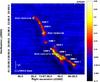 |
Fig. 1 LABOCA 870-μm image of the IRDC G304.74. The image is shown with linear scaling, and the colour bar indicates the flux density in units of Jy beam-1. The rms level is 0.03 Jy beam-1 (1σ). The first contour and the separation between contours is 3σ. The green plus signs show the submm peak positions, which were used as the line-observation target positions in the present study. The white circles indicate the nominal catalogue positions of the MSX 8-μm sources. The 1-pc scale bar and the effective LABOCA beam HPBW (~20″) are shown in the bottom left (modified from Paper I). |
The target cloud of the present study is the IRDC G304.74+01.32 (hereafter, G304.74). We recently mapped this IRDC in the 870-μm dust continuum emission with the LABOCA bolometer on APEX (Paper I). The cloud was found to have a integral-shaped/“hub-filament”-kind of structure (Myers 2009), and it was resolved into twelve clumps with the two-dimensional clumpfind algorithm (Williams et al. 1994). Four of the clumps were found to be associated with MSX 8-μm point-like sources, indicating embedded star formation. Moreover, three of these MSX-bright clumps are associated with IRAS point sources (the IRAS sources 13037-6112, 13039-6108, and 13042-6105; hereafter, IRAS 13037 etc.). Eight clumps in G304.74 were found to be dark in the MSX 8-μm image. The clump masses were estimated to be in the range ~40−220 M⊙ (assuming a dust temperature of 15 or 22 K), within the effective radii of ~0.3−0.5 pc. Unfortunately, G304.74 is not covered by the Spitzer infrared maps, which “only” cover the Galactic latitudes |b| ≤ 1°. Our 870-μm LABOCA map of G304.74 is shown in Fig. 1 (modified from Fig. 1 of Paper I). We also refer to Fig. 2 of Paper I for the MSX 8-μm image of the region overlaid with LABOCA contours.
To our knowledge, besides the IRDC identification of Simon et al. (2006) and our Paper I, the only studies of G304.74, or a clump within it, are those of Fontani et al. (2005) and Beltrán et al. (2006). The latter authors performed SIMBA 1.2-mm dust continuum mapping of the cloud, and identified eight clumps, including the MSX-bright sources (see our Paper I for more details). Fontani et al. (2005) carried out pointed CS and C17O observations towards one source in G304.74, namely IRAS 13039. By employing the Galactic rotation curve of Brand & Blitz (1993) and the radial velocity − 26.2 km s-1 derived from CS observations, Fontani et al. (2005) determined the source distance of 2.44 kpc. As discussed by Beuther et al. (2011), G304.74 constitutes a small part of the kpc-distance cloud complexes, which form a portion of the Coalsack dark cloud in the plane of the sky.
Source list.
Observed spectral-line transitions and observational parameters.
In the present paper, we present the first molecular-line observations along the whole filamentary structure of G304.74. These data are used to examine the basic physical properties of the cloud, such as the gas kinematics and dynamical state of the clumps. The cloud’s kinematic distance, and the distance-dependent parameters presented in Paper I, will also be revised. This study will also address some chemical properties of the clumps. For example, we investigate the amount of CO depletion, which has only recently been studied in IRDCs (Zhang et al. 2009; Hernandez et al. 2011; Miettinen et al. 2011; Chen et al. 2011).
The rest of this paper is structured as follows. The observations and data-reduction procedures are described in Sect. 2. The direct observational results are presented in Sect. 3. In Sect. 4/Appendix A, we describe the analysis and present the results of the physical and chemical properties of the cloud/clumps. Discussion of our results is presented in Sect. 5, and in Sect. 6 we summarise the main conclusions of this study.
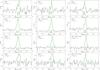 |
Fig. 2 Smoothed C17O(2−1) spectra. Overlaid on the spectra are the hf-structure fits. The relative velocities of individual hf components are indicated by vertical lines under the spectra. |
2. Observations and data reduction
The observations presented in this paper were made using the APEX 12-m telescope at Llano de Chajnantor (Chilean Andes). The telescope and its performance are described in the paper by Güsten et al. (2006). All the submm peak positions in G304.74 identified from our previous LABOCA 870-μm map were observed in C17O(2−1), and selected positions in the southern part of the filament were observed in 13CO(2−1), SiO(5−4), and CH3OH(5k − 4k) with the Swedish Heterodyne Facility Instrument (SHeFI; Belitsky et al. 2007; Vassilev et al. 2008a). The target positions with their physical properties are listed in Table 1. The observed transitions and observational parameters are listed in Table 2. The observations took place on 18–19 and 26–28 May 2011. As a frontend to the observations, we used the APEX-1 receiver of the SHeFI (Vassilev et al. 2008b). The backend to all observations was the Fast Fourier Transfrom Spectrometer (FFTS; Klein et al. 2006) with a 1 GHz bandwidth divided into 8192 channels.
The observations were performed in the wobbler-switching mode with a 150″ azimuthal throw (symmetric offsets) and a chopping rate of 0.5 Hz. The telescope pointing and focus corrections were checked by continuum scans of the planet Saturn, and the pointing was found to be better than ~5″. Calibration was done by means of the chopper-wheel technique, and the output intensity scale given by the system is  , which represents the antenna temperature corrected for atmospheric attenuation. The observed intensities were converted to the main-beam brightness temperature scale by
  , where ηMB is the main beam efficiency. The absolute calibration uncertainty is estimated to be around 10%.
The spectra were reduced using the CLASS90 programme of the IRAM’s GILDAS software package1. The individual spectra were averaged and the resulting spectra were Hanning-smoothed in order to improve the signal-to-noise ratio of the data. A first- or third-order polynomial was applied to correct the baseline in the final spectra. The resulting 1σ rms noise levels are ~40−100 mK at the smoothed resolutions.
The 13CO(2−1) and C17O(2−1) rotational lines contain three and nine hyperfine (hf) components, respectively. We fitted these hf structures using “method hfs” of CLASS90 to derive the LSR velocity (vLSR) of the emission, and full width at half maximum (FWHM) linewidth (Δv). The hf-line fitting can also be used to derive the line optical thickness, τ. However, in all spectra the hf components are blended together, thus the optical thickness could not be reliably determined. For the rest frequencies of the 13CO(2−1) hf components, we used the values from Cazzoli et al. (2004; Table 2 therein), whereas those for C17O(2−1) were taken from Ladd et al. (1998; Table 6 therein).
3. Observational results
The smoothed C17O(2−1) spectra towards all target positions are shown in Fig. 2. The line was clearly detected towards all sources, but its hf components are mostly blended in all cases. Towards a few sources, such as SMM 2, the hf structure is only partially resolved, but not sufficiently well to derive the line optical thickness. Figures 3–5 show the 13CO(2−1), SiO(5−4), and CH3OH(5k − 4k) spectra towards the observed five clumps in the southern part of the filament. All the 13CO(2 − 1) lines show a blue asymmetric profile, i.e., the blueshifted peak is stronger than the redshifted peak, and there is a self-absorption dip near the systemic velocity. The self-absorbed profiles of the 13CO lines indicate that the lines are optically thick. Moreover, the lines show non-Gaussian line-wing emission. In particular, SMM 2 shows high-velocity blueshifted wing emission up to −35 km s-1. The small “absorption”-like features seen in the 13CO spectra of SMM 4 and IRAS 13037 are caused by weak emission in the off-source reference position (off-beam). The line SiO(5 − 4) was detected only towards SMM 3, though the line is also very weak towards this source. In addition, we detected the DCN(3−2) line towards SMM 3 in the frequency band covering SiO(5−4) (see Fig. 6). The detected J = 3−2 rotational line of DCN is split into six hf components. In fitting this hf structure, we used the rest frequencies from the CDMS catalogue. The E-type methanol transition CH3OH(5−1,5−4 − 1,4)-E and the A-type transition CH3OH(50,5 − 40,4)-A+ at ~ 241.8 GHz were detected towards all the observed clumps. Moreover, towards SMM 2, a blend of CH3OH(54,1 − 44,0)-A+ and CH3OH(54,2 − 44,1)-A− was detected.
The spectral-line parameters derived from hf- and single Gaussian fits are given in Cols. (3)–(5) of Table 3. For the SiO(5−4) non-detections, we provide the 3σ upper limit to the line intensity. The integrated line intensities listed in Col. (6) of Table 3 were computed over the velocity range given in square brackets in the corresponding column. The quoted uncertainties in vLSR and Δv are formal 1σ fitting errors, whereas those in TMB and  also include the 10% calibration uncertainty. In the last column, we give the estimated peak line optical-thicknesses, which are derived in Sect. 4.3/Appendix A.3.
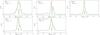 |
Fig. 3 Smoothed 13CO(2−1) spectra overlaid with hf-structure fits. The relative velocities of individual hf components are indicated by vertical lines under the spectra. The red vertical line shows the systemic velocity derived from C17O(2−1). |
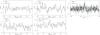 |
Fig. 4 Smoothed SiO(5−4) spectra. The line was detected only towards SMM 3 (overlaid with a Gaussian fit). Note that the spectrum towards SMM 3 is shown with a wider velocity range for reasons of clarity. |
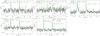 |
Fig. 5 Smoothed CH3OH(5k − 4k) spectra with Gaussian fits overlaid. In the spectrum towards SMM 2, the CH3OH(54,1 − 44,0)-A+ and CH3OH(54,2 − 44,1)-A− transitions are blended. Note that the velocity range shown is different for SMM 2 for reasons of clarity. |
Spectral-line parameters.
4. Analysis and results
4.1. Kinematic distance of G304.74+01.32
The LSR velocities derived from C17O(2−1) lie in the range vLSR ∈ [−27.4, −26.1] km s-1, i.e., within 1.3 km s-1. This velocity coherence shows that the filamentary IRDC G304.74 is a coherent structure, and not just a group of physically independent objects seen in projection on the plane of the sky.
The mean and median radial velocities derived from C17O(2−1) are −26.7 and −26.5 km s-1, respectively. To revise the cloud kinematic distance, we adopt the mean velocity of −26.7 km s-1, and employ the rotation curve of Reid et al. (2009). The resulting near kinematic distance, as expected to be appropriate for an IRDC seen in absorption, is d = 2.54 ± 0.66 kpc. The corresponding Galactocentric distance is about RGC ≃ 7.26 kpc (see Appendix A.1 for further details).
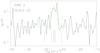 |
Fig. 6 The smoothed DCN(3 − 2) spectrum towards SMM 3. The line is overlaid with a hf-structure fit, and the vertical lines show the relative velocities of individual hf components. |
4.2. Revision of clump properties presented in Paper I
We used the revised cloud distance 2.54 ± 0.66 kpc to recalculate the distance-dependent clump parameters presented in Paper I, where the value d = 2.4 kpc was adopted. These parameters include the clump radius (R ∝ d), mass (M ∝ d2), and volume-averaged H2 number density ( ⟨ n(H2) ⟩ ∝ M/R3 ∝ d-1) (see Eqs. (6)–(8) in Paper I). The results are presented in Cols. (4)–(7) of Table 1. The revised values are in the ranges R ~ 0.3−0.5 pc, M ~ 40 − 250 M⊙, N(H2) ~ 1−3 × 1022 cm-2, and ⟨ n(H2) ⟩ ~ 0.3−1 × 104 cm-3. For more details, we refer to Appendix A.2.
Figure 7 shows the clump masses as a function of effective radius. A least squares fit to the data gives log (M) = (3.08 ± 0.23) + (2.82 ± 0.55)log (R), with the linear correlation coefficient r = 0.85. For comparison, we also show the mass-radius threshold for massive-star formation, M(R) = 870 M⊙ × (R/pc)1.33 inferred by Kauffmann & Pillai (2010).
4.3. Molecular column densities and fractional abundances
Details on how the molecular column densities and fractional abundances were calculated are given in Appendix A.3. In brief, we used Eq. (A.3) to estimate the peak optical thickness for those lines, which were used in the column-density calculations (see Col. (7) of Table 3). In all cases, the lines appear to be optically thin (τ0 ≪ 1). Therefore, the beam-averaged column densities of C17O, SiO, CH3OH, and DCN were calculated using Eq. (A.4). The fractional abundances of the molecules were calculated by dividing the molecular column density by the H2 column density. For this purpose, the values of N(H2) were derived from the LABOCA dust continuum map smoothed to the corresponding resolution of the line observations. The derived column densities and fractional abundances are listed in Table 4.
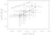 |
Fig. 7 Relation between mass and effective radius for the clumps in G304.74. The solid line shows the least squares fit to the data, i.e., log (M) ≈ 3.1 + 2.8log (R). The dotted line represents the mass-radius threshold for massive-star formation proposed by Kauffmann & Pillai (2010), i.e., M(R) = 870 M⊙ × (R/pc)1.33. |
Molecular column densities, fractional abundances with respect to H2, and CO depletion factors (fD).
4.4. CO depletion factors
To estimate the amount of CO depletion in the clumps, we calculated the CO depletion factors, fD, following the analysis outlined in Appendix A.4. The derived CO depletion factors, 0.3−2.3, are listed in Col. (4) of Table 4.
4.5. Gas kinematics and internal pressure
We used the measured C17O(2 − 1) linewidths to calculate i) the non-thermal portion of the line-of-sight velocity dispersion (averaged over a  beam), and ii) the level of internal turbulence (see below). The observed velocity dispersion is related to the FWHM linewidth as σobs = Δv/
 . The non-thermal velocity dispersion can then be calculated as (e.g., Myers et al. 1991)
  (1)where mC17O = 29 amu is the mass of the C17O molecule. Furthermore, the level of internal turbulence is given by fturb = σNT/cs, where cs is the one-dimensional isothermal sound speed (0.23 km s-1 in a 15 K H2 gas with 10% He, where the mean molecular weight per free particle is 2.33). The values of σNT and fturb are given in Cols. (2) and (3) of Table 5, respectively. The errors in these parameters were derived by propagating the errors in Δv and Tkin. In Fig. 8, we plot the FWHM linewidths as a function of clump effective radius (left panel), and the derived fturb values as a function of clump mass (right panel). The linewidths do not show any clear correlation with the clump size; they are, instead, scattered around a horizontal regression line (the fit is not shown), which suggests that the linewidths are more or less “constant” as a function of clump radius. As can be seen from the right panel of Fig. 8, the clumps are characterised by trans- to supersonic (σNT ≳ cs) non-thermal motions.
We also calculated the total (thermal + non-thermal) kinetic pressure within the clumps to be  (2)where ρ = 2.33mH ⟨ n(H2) ⟩ is the average gas-mass density of the clump, and mH is the mass of a hydrogen atom. The results, ~ 2 − 18 × 105 K cm-3 (6.7 × 10⁵ K cm-3 on average), are listed in Col. (4) of Table 5. We note that the pressures have considerable associated errors because of the assumed ± 5 K uncertainty in temperature.
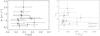 |
Fig. 8 Left: the FWHM linewidth of C17O(2 − 1) versus clump effective radius. Right: the σNT/cs ratio versus clump mass. The dashed line represents the limit between subsonic and supersonic non-thermal motions, i.e., σNT/cs = 1. |
The clump virial masses and virial parameters, and the estimated external pressure required to bring the clump into virial equilibrium.
4.6. Virial analysis
To examine the dynamical state of the clumps, we calculated their virial masses by ignoring the effects of external pressure, rotation, and magnetic field in using the formula 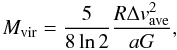 (3)where Δvave is the width of the spectral line emitted by the molecule of mean mass μ = 2.33, and G is the gravitational constant. The parameter a = (1 − p/3)/(1−2p/5), where p is the power-law index of the density profile [n(r) ∝ r − p], is a correction for deviations from uniform density (Bertoldi & McKee 1992, hereafter, BM92, their Appendix A). In the clump’s gravitational potential energy, the a parameter appears as
 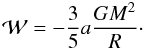 (4)We note that the effect of the clump’s ellipticity is neglected here (see BM92). We adopted the value p = 1.6 (a = 1.3) found by Beuther et al. (2002) for a sample of high-mass star-forming clumps. As a function of the observed linewidth, Δvobs, Δvave is given by (Fuller & Myers 1992)
 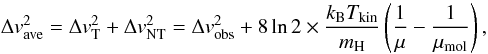 (5)where ΔvT is the thermal linewidth, μ = 2.33, and μmol = 29 for C17O, which is the molecule that we employed in the analysis. The virial masses are listed in Col. (2) of Table 6. The associated error was propagated from those of R, Δvobs, and Tkin.
The virial parameters of the clumps were calculated following the definition by BM92, i.e.,  (6)where
  is the internal kinetic energy of the clump. The value αvir = 1 corresponds to the virial equilibrium, i.e.,
  . The value αvir ≤ 2 corresponds to the self-gravitating limit defined by
  (e.g., Pound & Blitz 1993)2. The derived αvir values are given in Col. (3) of Table 6. The uncertainty was derived by propagating the errors in both mass estimates.
The derived αvir values, ~ 0.4 − 2.8, are plotted as a function of the clump mass in Fig. 9. Although the αvir values are associated with considerable uncertainties, most of the clumps appear to be gravitationally bound, and some of them are close virial equilibrium. Moreover, there is a hint of a negative correlation between αvir and M. A least squares fit to the data points yields log (αvir) = (1.38 ± 0.63) − (0.69 ± 0.32)log (M), with the correlation coefficient r = −0.56.
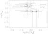 |
Fig. 9 Relation between virial parameter and mass for the clumps in G304.74. The solid line is the least squares fit to the data, i.e., log (αvir) ≃ 1.4 − 0.7log (M). The dashed line indicates the virial-equilibrium limit of αvir = 1, and the dash-dotted line shows the limit of gravitational boundedness or αvir = 2. |
4.7. The confining effect of external pressure
The slope of the αvir − M relation found
above, –0.69, is quite close to the value −2/3 ≃ −0.67 that is characteristic of
pressure-confined clumps (BM92). Therefore, the external pressure may play an important
role in the dynamics of the clumps. Taking the kinetic energy resulting from the surface
pressure on the clump,  , into account, we can write the virial theorem in the
form (e.g., McKee & Zweibel 1992)3
, into account, we can write the virial theorem in the
form (e.g., McKee & Zweibel 1992)3 (7)The above energies can be written as a function of
pressure as
(7)The above energies can be written as a function of
pressure as  and
and  (10)In the above formulae,
  is the clump volume, Pext
is the external pressure on the clump, and Pgrav is the
gravitational pressure. We can write Pgrav as
is the clump volume, Pext
is the external pressure on the clump, and Pgrav is the
gravitational pressure. We can write Pgrav as 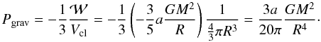 (11)Substituting Eqs. (8)–(10) into Eq. (7), we get
  (12)From Eq. (12), we can estimate the Pext required to bring the
clumps into virial equilibrium, which is roughly suggested by Fig. 9. The estimated
(12)From Eq. (12), we can estimate the Pext required to bring the
clumps into virial equilibrium, which is roughly suggested by Fig. 9. The estimated  values are listed in Col. (4) of Table 6. We note that the values are associated with very
large errors, and we only give the central values in the table. The clumps SMM 1–4 in the
southern filament are formally characterised by negative external pressures. Although
there are large uncertainties in the analysis, these clumps should be either warmer or
have some additional internal pressure acting outward, such as magnetic pressure, in order
to achieve virial equlibrium. The positive values of are found for the clumps north of SMM 4, to lie in the
range ~ 0.5 − 12 × 105 K cm-3
(~3.3 × 10⁵ K cm-3 on average).
values are listed in Col. (4) of Table 6. We note that the values are associated with very
large errors, and we only give the central values in the table. The clumps SMM 1–4 in the
southern filament are formally characterised by negative external pressures. Although
there are large uncertainties in the analysis, these clumps should be either warmer or
have some additional internal pressure acting outward, such as magnetic pressure, in order
to achieve virial equlibrium. The positive values of are found for the clumps north of SMM 4, to lie in the
range ~ 0.5 − 12 × 105 K cm-3
(~3.3 × 10⁵ K cm-3 on average).
4.8. Mass infall
The detected 13CO(2 − 1) lines, most notably towards SMM 2, show the “classic” signature of the infalling gas motions, i.e., redshifted absorption dips, or blue asymmetric profiles (e.g., Lucas 1976; Myers et al. 1996). The optically thin C17O lines peak close to the radial velocity of the self-absorption dip. Therefore, we can presume that the double-peak profiles are not caused by two distinct velocity components along the line of sight. We note, however, that many of the absorption features are slightly redshifted with respect to the systemic velocity (Fig. 3). The blue asymmetry is weakest towards SMM 1, which indicates that in this clump there is the slowest infalling gas. We estimated the infall velocity, Vinf, using Eq. (9) of Myers et al. (1996)
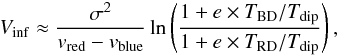 (13)where σ is the velocity dispersion
derived from the appropriate optically thin line (we used the C17O lines),
vred − vblue is the difference
between the radial velocities of the red and blue peaks, TBD
and TRD are the heights of the blue and red peaks above the
absorption dip, and Tdip is the intensity of the absorption
dip (see also Fig. 2 of Myers et al. 1996, for the definitions). The obtained values,
~ 0.03−0.20 km s-1, are listed in Col. (2) of Table 7. The uncertainty in Vinf
was estimated from the error in the FWHM linewidth of C17O(2 − 1).
(13)where σ is the velocity dispersion
derived from the appropriate optically thin line (we used the C17O lines),
vred − vblue is the difference
between the radial velocities of the red and blue peaks, TBD
and TRD are the heights of the blue and red peaks above the
absorption dip, and Tdip is the intensity of the absorption
dip (see also Fig. 2 of Myers et al. 1996, for the definitions). The obtained values,
~ 0.03−0.20 km s-1, are listed in Col. (2) of Table 7. The uncertainty in Vinf
was estimated from the error in the FWHM linewidth of C17O(2 − 1).
Assuming spherically symmetric infall, and that the mass contained in the spherical shell is dM(r) = 4πr2ρdr, the infall velocities can be used to estimate the mass infall rate as
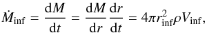 (14)where rinf is the size of the
infalling region (taken to be the clump effective radius), and
ρ = 2.33mH ⟨ n(H2) ⟩
is again the average gas mass density4. The derived
values, ~2−36 × 10-5 M⊙ yr-1, with
uncertainties estimated from the errors in Vinf, are given in
Col. (3) of Table 7.
(14)where rinf is the size of the
infalling region (taken to be the clump effective radius), and
ρ = 2.33mH ⟨ n(H2) ⟩
is again the average gas mass density4. The derived
values, ~2−36 × 10-5 M⊙ yr-1, with
uncertainties estimated from the errors in Vinf, are given in
Col. (3) of Table 7.
Assuming that Ṁinf remains constant, the infall timescale can
be calculated from  (15)The obtained timescales, ~6−46 × 105 yr,
are listed in Col. (4) of Table 7 (the uncertainty
is based on that in Ṁinf).
(15)The obtained timescales, ~6−46 × 105 yr,
are listed in Col. (4) of Table 7 (the uncertainty
is based on that in Ṁinf).
We also calculated the free-fall velocities of the clumps  (16)which were then compared with the derived infall velocities. In the last column of Table 7, we list the Vinf/Vff ratios. The associated uncertainty was propagated from those of Vinf, M, and R. In all cases, the infall velocity is much lower than the corresponding free-fall velocity.
Mass-infall parameters.
4.9. Fragmentation and stability analysis of the filament
The IRDC G304.74 is highly filamentary in shape, its total mass being about ~1200 M⊙ (the sum of all clump masses), and it is resolved into twelve submm clumps at ~20″ resolution. The projected linear extent of filament’s long axis is about 12′ or 8.9 pc, and the filament’s mass per unit length, or line mass, is Mline ≃ 135 M⊙ pc-1. We note that this line mass may only represent a lower limit, because there is likely to be a lot of mass on larger scales (Kainulainen et al. 2011b). The projected separations between the clump submm peak positions lie in the range 22″−115″, or 0.27–1.42 pc at the cloud distance (61″ = 0.75 pc on average). The shortest separations are found near SMM 6 and IRAS 13037, whereas the separations are largest around SMM 7.
To examine the fragmentation of G304.74 in more detail, we first calculate its thermal
Jeans length from  (17)where cs was adopted to be
0.23 km s-1 (Sect. 4.5),
Σ0 = 2.33mHN(H2) is
the surface density, and N(H2) refers to the central column
density for which we use the median value ~1.4 × 1022 cm-2
(see Col. (6) of Table 1). The resulting thermal
Jeans length is only ~0.05 pc, which is about five times less than the spatial
resolution of our LABOCA map, and therefore much shorter than the observed minimum clump
separation. Thermal Jeans instability does not appear to be responsible for the cloud
fragmentation on the scale of clumps.
(17)where cs was adopted to be
0.23 km s-1 (Sect. 4.5),
Σ0 = 2.33mHN(H2) is
the surface density, and N(H2) refers to the central column
density for which we use the median value ~1.4 × 1022 cm-2
(see Col. (6) of Table 1). The resulting thermal
Jeans length is only ~0.05 pc, which is about five times less than the spatial
resolution of our LABOCA map, and therefore much shorter than the observed minimum clump
separation. Thermal Jeans instability does not appear to be responsible for the cloud
fragmentation on the scale of clumps.
On the other hand, we found that the filament is dominated by supersonic non-thermal
motions. Therefore, it may be appropriate to replace cs in
Eq. (17) with the effective sound speed,
which takes both thermal and non-thermal motions into account, i.e.,  , where σNT, 3D is the
three-dimensional non-thermal velocity dispersion (e.g., Chandrasekhar 1951; Bonazzola et al.
1987). Here we have assumed isotropic non-thermal motions, i.e.,
, where σNT, 3D is the
three-dimensional non-thermal velocity dispersion (e.g., Chandrasekhar 1951; Bonazzola et al.
1987). Here we have assumed isotropic non-thermal motions, i.e.,  . Using the median value of
σNT, 1D = 0.47 km s-1 (see Col. (2) of
Table 5), the effective, or “turbulent” Jeans
length becomes ~0.24 pc. This is about five times larger than the thermal Jeans
length, but still much smaller than the average clump separation of ~0.75 pc.
Therefore, the observed fragmentation of the filament cannot be attributed either to
non-thermal Jeans-type instability.
. Using the median value of
σNT, 1D = 0.47 km s-1 (see Col. (2) of
Table 5), the effective, or “turbulent” Jeans
length becomes ~0.24 pc. This is about five times larger than the thermal Jeans
length, but still much smaller than the average clump separation of ~0.75 pc.
Therefore, the observed fragmentation of the filament cannot be attributed either to
non-thermal Jeans-type instability.
According to the magnetohydrodynamic “sausage”-instability theory, fragmentation of a
self-gravitating fluid cylinder will lead to the formation of distinct condensations with
almost periodic separations. This fragmentation length-scale corresponds to the wavelength
at which the instability grows the fastest (e.g., Chandrasekhar & Fermi 1953; Nagasawa
1987; see also Jackson et al. 2010). If
the cylinder’s radius is Rcyl, then, for an incompressible
fluid, perturbation analysis shows that the above critical wavelength is  . If we use as Rcyl the mean
clump effective radius of ~0.4 pc, we obtain
. If we use as Rcyl the mean
clump effective radius of ~0.4 pc, we obtain  pc. This is clearly a longer length scale than observed
in G304.74. On the other hand, for an isothermal, infinitely long gas cylinder the fastest
growing mode appears at
pc. This is clearly a longer length scale than observed
in G304.74. On the other hand, for an isothermal, infinitely long gas cylinder the fastest
growing mode appears at  , where
H = cs/
, where
H = cs/ is the isothermal scale height with
ρ0 the central gas mass density along the axis of the
cylinder (e.g., Nagasawa 1987). If we compute
ρ0 assuming that the central number density is
105 cm-3, we obtain the scale height
H = 0.013 pc, and thus
is the isothermal scale height with
ρ0 the central gas mass density along the axis of the
cylinder (e.g., Nagasawa 1987). If we compute
ρ0 assuming that the central number density is
105 cm-3, we obtain the scale height
H = 0.013 pc, and thus  pc. This is comparable to the effective Jeans-length
calculated above. If the value of H is calculated using the effective
sound speed, ceff, i.e., we calculate the effective scale
height, we get Heff = 0.03 pc, and
pc. This is comparable to the effective Jeans-length
calculated above. If the value of H is calculated using the effective
sound speed, ceff, i.e., we calculate the effective scale
height, we get Heff = 0.03 pc, and  pc. This wavelength is close to the observed average
clump separation. We also note that it is comparable to the average width of the filament,
~0.8 pc, in accordance with the theory (Nakamura
et al. 1993).
pc. This wavelength is close to the observed average
clump separation. We also note that it is comparable to the average width of the filament,
~0.8 pc, in accordance with the theory (Nakamura
et al. 1993).
We next examine whether the G304.74 filament could be susceptible to axisymmetric
perturbations or radial collapse. For an unmagnetised, infinite, isothermal filament, the
instability is reached if its Mline value exceeds the critical
equilibrium value of  (e.g., Ostriker
1964; Inutsuka & Miyama 1992). At
Tkin = 15 K, the critical value is
(e.g., Ostriker
1964; Inutsuka & Miyama 1992). At
Tkin = 15 K, the critical value is  M⊙ pc-1. Using
this value, we estimate that the ratio
M⊙ pc-1. Using
this value, we estimate that the ratio  for G304.74. Thus, G304.74 appears to be a thermally
supercritical filament susceptible to fragmentation, in agreement with the detected clumpy
structure. If the external pressure is not negligible, as may be the case for G304.74,
then
for G304.74. Thus, G304.74 appears to be a thermally
supercritical filament susceptible to fragmentation, in agreement with the detected clumpy
structure. If the external pressure is not negligible, as may be the case for G304.74,
then  is actually smaller than the above value (e.g., Fiege & Pudritz 2000a), making the filament even
more supercritical. However, owing to the presence of non-thermal motions, it may be
appropriate to replace with the virial mass per unit length,
is actually smaller than the above value (e.g., Fiege & Pudritz 2000a), making the filament even
more supercritical. However, owing to the presence of non-thermal motions, it may be
appropriate to replace with the virial mass per unit length,  , where ⟨ σ2 ⟩ is the
square of the total velocity dispersion obtained from Eq. (5) as
, where ⟨ σ2 ⟩ is the
square of the total velocity dispersion obtained from Eq. (5) as  (Fiege & Pudritz
2000a). Using again the value Tkin = 15 K and the
C17O linewidths, we obtain the mean velocity dispersion of
⟨ σ2 ⟩ 1/2 = 0.54 km s-1. This leads
to the values
(Fiege & Pudritz
2000a). Using again the value Tkin = 15 K and the
C17O linewidths, we obtain the mean velocity dispersion of
⟨ σ2 ⟩ 1/2 = 0.54 km s-1. This leads
to the values  M⊙ pc-1 and
  . In this case, G304.74 as a whole would be near virial
equilibrium. The fragmentation timescale for a filament of radius
Rcyl is expected to be comparable to its radial signal
crossing time,
τcross = Rcyl/ ⟨ σ2 ⟩ 1/2
(see Eq. (26) in Fiege & Pudritz 2000b), which
for G304.74 is estimated to be ~ 7.2 × 10⁵ yr. We note that the value of
⟨ σ2 ⟩ 1/2, and thus
. In this case, G304.74 as a whole would be near virial
equilibrium. The fragmentation timescale for a filament of radius
Rcyl is expected to be comparable to its radial signal
crossing time,
τcross = Rcyl/ ⟨ σ2 ⟩ 1/2
(see Eq. (26) in Fiege & Pudritz 2000b), which
for G304.74 is estimated to be ~ 7.2 × 10⁵ yr. We note that the value of
⟨ σ2 ⟩ 1/2, and thus  , may increase if the cloud’s gravitational potential
energy is converted into gas kinetic energy during the contraction of the cloud. We also
note that in the case of a magnetised molecular-cloud filament, the critical mass per unit
length is unlikely to differ from that of an unmagnetised filament by more than a factor
of order unity (Fiege & Pudritz 2000a,b).
, may increase if the cloud’s gravitational potential
energy is converted into gas kinetic energy during the contraction of the cloud. We also
note that in the case of a magnetised molecular-cloud filament, the critical mass per unit
length is unlikely to differ from that of an unmagnetised filament by more than a factor
of order unity (Fiege & Pudritz 2000a,b).
5. Discussion
5.1. Fragmentation and dynamical state of G304.74+01.32
The average projected clump separation in G304.74 is about 0.75 pc. As shown above, this value can be explained if the fragmentation of the parent filament is caused by a “sausage”-type (or pinch) instability, where the dominant unstable mode appears at the wavelength depending on the effective sound speed. This instability might have been triggered by, e.g., an increase in the radial inward force or a radial contraction leading to an increase in the tension force of the azimuthal magnetic field. This conforms to the results of Jackson et al. (2010), who speculated that the “sausage”-type instability is the main physical driver of the fragmentation of filamentary IRDCs. Henning et al. (2010) and Kang et al. (2011) found that the mean clump separation is 0.9 pc in both the filamentary IRDC G011.11-0.12 or the Snake, and IRDC G049.40-00.01, respectively. This resembles the situation in G304.74, and could therefore be indicative of a similar fragmentation process. In Paper I, we discussed the possibility that the origin of the G304.74 filament, and its fragmentation into clumps is caused by supersonic turbulent flows. Even though the formation of the cloud might have been caused by converging turbulent flows, the role of random turbulence in fragmenting the filament appears unclear in the light of the present results. Nevertheless, our new results here support the importance of non-thermal motions in G304.74.
The slope of the αvir–M relation that we found is roughly consistent with the prediction of BM92 for clumps confined by ambient pressure from their surrounding medium, i.e., αvir ∝ M−2/3. This slope can be understood as follows. On the one hand, the clump mass was found to be roughly proportional to R3 (Fig. 7). On the other hand, the linewidth-radius “relation” shown in Fig. 8 is roughly flat, i.e., Δv ≈ const. Therefore, from Eqs. (3) and (6) we see that αvir ∝ RΔv2/M ∝ M1/3M-1 ∝ M − 2/3. Although our clumps, or most of them, appear to be gravitationally bound (αvir ≤ 2), it is possible that the ambient pressure (still) plays a non-negligible role in the clump dynamics. We note that for real pressure-confined clumps, αvir ≫ 1, and the clumps are not gravitationally bound (BM92).
Could the external pressure be caused by turbulent flow motions outside the cloud? To estimate the turbulent ram pressure,  , we use the average 13CO(2−1) linewidth of ~2.2 km s-1 derived for five of our clumps, and assume the density of the 13CO emitting gas to be 103 cm-3 (following Lada et al. 2008). If Tkin is in the range 10–20 K, the corresponding non-thermal velocity dispersion is σNT ≃ 0.93 km s-1, which yields the value Pram/kB ~ 3 × 10⁵ K cm-3. This is only about two times lower than the average internal kinetic pressure within the clumps, and very close to the average external pressure required for virial equilibrium (
 ; Sect. 4.7). Therefore, this supports the scenario of the importance of turbulence presented in Paper I. The obtained Pram/kB value is also consistent with intercloud pressures of 104−106 K cm-3 deduced from theoretical estimates and different observations (see Field et al. 2011, and references therein). However, we note that the large-scale turbulent motions are anisotropic, and therefore that the associated pressure may be unable to confine the cloud, but could rather distort and/or even disrupt it (e.g., Ballesteros-Paredes 2006). The finding that for the G304.74 filament suggests that it is close to virial equilibrium. The virial balance may be difficult to explain in the context of the turbulent fragmentation discussed in Paper I, because turbulent motions are expected to induce a flux of mass, momentum, and energy between the cloud and its surrounding medium (Ballesteros-Paredes 2006). In addition, the detection of large-scale infall motions towards G304.74 suggests it to be out-of-equilibrium. For comparison, the Herschel study of the Aquila rift and Polaris Flare regions by André et al. (2010) showed that practically all filaments with
  were associated with prestellar cores and/or embedded protostars. On the other hand, filaments with
  were generally found to lack such star-formation signatures. More observations of higher resolution would be needed to characterise more clearly the star-formation activity in G304.74, and compare it with the filamentary structures revealed by Herschel.
If the  ratio is indeed ≃1, then from Eq. (11) of Fiege & Pudritz (2000a), and the average ratio of the external to internal pressure of
 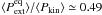 , we estimate that the ratio of the total magnetic to kinetic energies per unit length is
  . This value is > 0, and therefore suggests that i) the overall effect of the magnetic field on the cloud is to provide support; and ii) the magnetic field is poloidally dominated. This disagrees with Fiege & Pudritz (2000a), who found that the magnetic fields in the filamentary clouds that they analysed are likely to be helical and toroidally dominated. However, Fiege et al. (2004) analysed the Snake IRDC, which is more similar to G304.74, and concluded that it is likely dominated by the poloidal component of the magnetic field (or magnetically neutral), and therefore an excellent candidate for a magnetically supported filament. This may also be the case for the G304.74 filament. Interestingly, Fiege & Pudritz (2000b) found that models with purely toroidal fields remain stable in “sausage” modes, whereas models with a poloidal field component may be unstable. We note, however, that the observed fragmentation of the filament strongly suggests that the magnetic field is not purely poloidal (or toroidal), because otherwise the fragmentation would have presumably been stabilised (Fiege & Pudritz 2000b). If the filament fragmentation were caused by sausage-type instability, some toroidal magnetic field would probably needed, because the magnetic pressure associated with the poloidal field would resist the “squeezing” of the cloud.
On the other hand, the ambient pressure can also arise from the cloud’s self-gravity. This was found to be the case for the Pipe Nebula by Lada et al. (2008), who found all the cores within the cloud to have αvir > 1, and αvir ∝ M-0.66. The pressure due to the weight of the cloud is 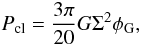 (18)where Σ = M/πR2 is the mean mass surface density of the cloud, and φG is a dimensionless correction factor apllied to account for the non-spherical geometry of a cloud (BM92; cf. our Eq. (11)). Following BM92, we use as the mean effective cloud radius the value
 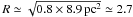 pc, where 0.8 pc is the average width of the filament. The corresponding surface density is Σ ≃ 1 g cm-2. The aspect ratio of the filament is about y ≃ 8.9 pc/0.8 pc ~ 11 (prolate), hence we adopt the value φG ≃ 2 (see Appendix B of BM92). Thus, we obtain the value Pcl ~ 5.5 × 10⁴ K cm-3. This is about an order of magnitude lower than the average internal kinetic pressure within the clumps or the average value, suggesting that the cloud’s weight does not contribute significantly to the overall confining pressure. We note, however, that Kainulainen et al. (2011b) found that the masses of IRDCs traced by the thermal dust emission are generally only ≲ 10 − 20% of the masses traced by near-infrared and CO data. Therefore, the pressure due to the weight of the cloud itself, which is mostly caused by the material at low column densities, is likely to be higher than estimated above.
Some of the clumps at the southern end of the filament were found to be characterised by negative external pressures in the case of virial equilibrium (or “energy equipartition”; Sect. 4.7), suggesting that they should be either warmer or have some additional internal pressure. Interestingly, this conforms to the results obtained in Paper I, where we used the dust opacities at 8 μm and 870 μm to estimate the dust temperatures towards the MIR-dark submm peaks. The clumps SMM 1 and 2 in the southern tip of the filament were estimated to have temperatures of ~30 K, but the values were associated with very large relative errors of ~60−70% (thus we adopted Tdust = 15 K). The masses (mean densities) of SMM 1 and 2 would be ~44 M⊙ (0.2 × 104 cm-3) and 22 M⊙ (0.3 × 104 cm-3), respectively, if we assumed that Tdust = 30 K. The non-thermal velocity dispersions would be 0.27 and 0.23 km s-1, and the total kinetic pressures about 1.2 × 10⁵ K cm-3 and 1.6 × 10⁵ K cm-3, respectively. Consequently, the external pressures required to virial balance would become positive, i.e.,  and ~1.1 × 10⁵ K cm-3, for SMM 1 and 2, respectively. These are in reasonable agreement with the values estimated towards other clumps (see Col. (4) of Table 6). The present results seem to support the possibility of a north-to-south temperature gradient of ~15 → 30 K in G304.74.
5.2. Clump kinematics, infall motions, and prospects for massive-star formation
The clumps in G304.74 appear to be characterised by transonic to supersonic internal non-thermal motions. According to the turbulent core model of McKee & Tan (2003), the clump (or core) has to be supersonically turbulent in order to achieve a high mass-accretion rate and be able to form massive stars. The presence of this turbulence is also expected to lead to the formation of substructure within the clump. Higher-resolution observations would be needed to find out whether the clumps have fragmented into smaller cores. For example, interferometric observations of a sample of clumps associated with IRDCs have revealed embedded cores within them (e.g., Rathborne et al. 2008; Hennemann et al. 2009; Wang et al. 2011).
The clump SMM 6, which has the second largest fturb value (~3), is associated with two MSX point sources, suggesting that it indeed hosts subfragments, and that they have already been collapsed. On the other hand, as shown in Fig. 7, none of the clumps appear to clearly fullfil the mass-radius threshold for massive-star formation proposed by Kauffmann & Pillai (2010). Only within the uncertainties could the two most massive clumps, SMM 3 and 4, exceed this limit.
The supersonic “turbulent” motions in the clumps may be due to gravitational infall motions (see Heitsch et al. 2009, and references therein). Evidence of large-scale infall motions in 13CO lines was indeed found towards the southern clumps (see further discussion below). If the whole filament is in the process of hierarchical gravitational collapse with clumps collapsing locally, a complex velocity pattern is expected to be created. This “turbulence” is unable to resist gravitational collapse; it is instead generated from the collapse itself (Ballesteros-Paredes et al. 2011).
Radiative transfer models have shown that if the clump centre collapses faster than the outer layers, the observed spectral line should have two peaks with the blueshifted peak being stronger than the redshifted one (Zhou et al. 1993; Myers et al. 1996). The blue peak originates from the rear side of the clump, whereas the red peak comes from the front part of the clump. The central dip between the two peaks is caused by the envelope layer (see also Evans 1999). Similar line profiles have been seen towards SMM 1–4 and IRAS 13037, and are therefore likely undergoing large-scale inward motions. We derived the infall velocites and mass infall rates of ~0.03−0.20 km s-1 and ~2−36 × 10-5 M⊙ yr-1, respectively. These are comparable to the values 0.14 km s-1 and 3 × 10⁻⁵ M⊙ yr-1 found by Hennemann et al. (2009) towards J18364 SMM 1 South, which is a massive clump within an IRDC. Chen et al. (2010) measured higher infall velocities and rates of ~0.7−4.6 km s-1 and ~1−28 × 10-3 M⊙ yr-1, respectively, for their sample of MYSOs associated with extended green objects (EGOs) and IRDCs. Typically, the mass infall rates in MYSOs are ~10-4 − 10-2 M⊙ yr-1 (e.g., Klaassen & Wilson 2007; Zapata et al. 2008; Beltrán et al. 2011). We note that the infall timescales we derived, ~6−46 × 105 yr, are quite long compared to the characteristic timescale of ~105 yr for high-mass star formation (e.g., Davies et al. 2011, and references therein). The infall rate, however, may not remain constant during the star-formation process, which could also explain some of the large observed variations in the values quoted above.
We found that the infall velocities are one to two orders of magnitude lower than expectations for a free-fall collapse. This suggests that the large-scale collapse is not gravitationally dominated, but might be retarded by, e.g., magnetic fields. The predominantly poloidal magnetic field could resist motions perpendicular to the poloidal field lines, such as appears to be the case in the Snake IRDC (Fiege & Pudritz 2000b; Fiege et al. 2004). We also emphasise that the derived infall parameters refer to the infall of the surrounding gas onto a (pre-)protocluster, not onto individual stars. For example, the timescale for (disk) accretion from the infalling envelope may be substantially shorter than the infall timescale. The current data do not allow us to decide whether the observed large-scale mass infall could feed competitive accretion in the clumps/protoclusters (Bonnell & Bate 2006), or be related to monolithic collapse leading to massive star formation (McKee & Tan 2003). On the one hand, the formation of high-mass stars in G304.74 seems uncertain according to the mass-radius threshold proposed by Kauffmann & Pillai (2010). On the other hand, the high luminosites of the IRAS sources 13 037 and 13 039, ~1.5−2 × 10³ L⊙ (Paper I), shows that at least intermediate-mass star- and/or cluster formation is taking place in this IRDC.
5.3. The observed chemical properties of the clumps
5.3.1. CO depletion and the SiO detection towards SMM 3
The CO depletion factors we derived are in the range fD ~ 0.3 − 2.3. Therefore, CO molecules do not appear to be significantly depleted on the scale of clumps in G304.74, which conforms to the low average H2 densities. Higher-resolution observations would be needed to investigate whether the clumps contain smaller and more CO-depleted cores. The values fD < 1 could be due to too small a canonical CO abundance being used, or contamination of non-depleted gas along the line of sight (see also Miettinen et al. 2011, and references therein). The latter possibility, however, may be less important because the cloud is located above the Galactic plane, and thus relatively free of contaminating emission along the line of sight. Uncertainties in N(H2), particularly due to the dust opacity, propagate of course into those of x(C17O) and fD.
It is unsurprising that we found no evidence of CO freeze-out towards the IRAS sources and SMM 6, which are all MIR bright and very likely associated with ongoing star formation. The physical processes associated with star-formation activity, such as outflows, heating, etc., are expected to release CO from the icy grain mantles back into the gas phase. The largest fD values are seen consistently towards the MIR-dark clumps SMM 1 and 3. However, the detection of SiO emission in SMM 3 implies that there are outflows, because gas-phase SiO is expected to be produced when shocks disrupt the dust grains (e.g., Hartquist et al. 1980; Schilke et al. 1997). This agrees with the finding of Sakai et al. (2010, henceforth, SSH10), i.e., that the fraction of shocked gas (as traced by SiO) is higher in the MSX-dark sources than in the MSX-bright sources. This could indicate that the MIR-dark clumps are associated with newly formed shocks giving rise to stronger SiO emission, whereas the weaker emission from the MIR-bright clumps could be due to shocks being older, and thus milder. We note that the highest estimated SiO column density value in SMM 3, ~2.5 × 1013 cm-2, is comparable to the values ~1.1−2.6 × 1013 cm-2 found by SSH10 towards their MSX-dark clumps.
In contrast, Hernandez et al. (2011) found depletion factors of up to fD ~ 5 in the highly filamentary IRDC G035.39-00.33. Miettinen et al. (2011) derived the values fD ~ 0.6−2.7 towards a sample of clumps within different IRDCs, which are very similar to those obtained in the present work with the same telescope/angular resolution. Higher values of fD ~ 6−19 were found by Chen et al. (2011) for their sample of high-mass star-forming clumps, including sources within IRDCs, using the 10-m SMT observations of C18O at 34″ resolution. This shows that strong CO depletion is possible even on the scale of clumps. We note that Hernandez et al. (2011) used the CO depletion timescale to constrain the lifetime of G035.39-00.33 (or the part of the cloud showing the strongest depletion). These investigations are useful considering the cloud formation timescales and mechanisms. Unfortunately, since we found no clear evidence of CO depletion in G304.74, we were unable to perform similar analysis.
5.3.2. CH3OH
The fractional CH3OH abundances in the observed clumps were estimated to lie in the range ~0.2−12 × 10-9. The lowest values are found towards the MIR-dark clump SMM 2, and the highest ones towards SMM 3 and IRAS 13037.
The pure gas-phase chemical models suggest that CH3OH is formed from methylium cation through the radiative association reaction  , followed by the electron recombination reaction
  . The latter reaction is, however, too inefficient to explain the observed CH3OH abundances in star-forming regions alone (see, e.g., Wirström et al. 2011, and references therein). For example, the CH3OH observations performed by van der Tak et al. (2000) towards a sample of 13 massive young stellar objects (MYSOs) suggested three types of abundance profiles: the coldest sources have CH3OH abundances of ~10-9, warmer sources are characterised by a range of abundances from ~10-9 to ~10-7, and the hot cores have x(CH3OH) ~ 10-7. These high abundances indicate that solid CH3OH must have been evaporated from the icy grain mantles into the gas phase. In the grain-surface chemistry scheme, CH3OH is formed through successive hydrogenation of CO onto dust grains (CO → HCO → H2CO → CH2OH → CH3OH), and subsequent grain mantle evaporation is then predicted to cause the gas-phase abundance of CH3OH to be > 10-8 (e.g., van der Tak et al. 2000; Charnley et al. 2004; Garrod et al. 2008). In addition to grain heating, methanol can be released from grain mantles by moderate shocks (e.g., Bachiller & Perez Gutierrez 1997, and references therein).
The methanol abundances derived in the present work, that is the lowest values found in SMM 2, do not appear to necessarily require mantle evaporation (see below). The detection of high-velocity 13CO wing emission in SMM 2, however, suggests the presence of outflow activity. The rest of the x(CH3OH) values, particularly in SMM 3 and IRAS 13037, appear to imply that CH3OH has been injected from dust grains into the gas. In SMM 3, the high CH3OH abundance together with the SiO detection and 13CO wing emission, are likely related to outflow activity. The latter wing-emission signature was also found towards IRAS 13037, but the SED of this source is indicative of hot dust (Paper I). Therefore, in addition to grain processing in shocks, the central YSO(s) may have raised the dust temperature above 100 K in IRAS 13037, which is the approximate sublimation temperature of CH3OH (e.g., Garrod & Herbst 2006). Interestingly, besides the highest CH3OH abundance, the strongest CO depletion was found towards SMM 3. This could be a sign of enhanced methanol production in SMM 3 caused by CO freeze-out (e.g., Whittet et al. 2011, and references therein); we still see a remnant of stronger CO depletion where CO hydrogenation on dust grains has occurred, as well as the product of this process, i.e., the gas-phase CH3OH.
Additional CH3OH observations towards IRDCs have been done by other authors. Beuther & Sridharan (2007) studied a sample of massive clumps within IRDCs, and measured CH3OH column densities and abundances of 1.7−37.2 × 1013 cm-2 and 0.4−10.7 × 10⁻¹⁰, respectively. Although their column densities are very similar to our values, our abundances are generally higher. As discussed by Beuther & Sridharan (2007), their average CH3OH abundance of 4.3 × 10⁻¹⁰ is similar to the CH3OH abundances of 6 × 10⁻¹⁰ found in the low-mass starless cores L1498 and L1517B by Tafalla et al. (2006). There are no internal heating/outflows in starless cores, hence grain processing is unexpected in these sources. Sakai et al. (2010) derived CH3OH column densities in the range <2.9−24.8 × 1014 cm-2 towards a sample of 20 massive clumps within IRDCs, which are much higher than those found in the present work. Sakai et al. (2010) pointed out that their much higher N(CH3OH) values than to those of Beuther & Sridharan (2007) could be due to the source selection criteria; SSH10 studied MSX-dark clumps with signatures of star-formation activity. On the basis of the observed correlation between the CH3OH and SiO abundances, SSH10 concluded that the origin of CH3OH in the MSX-dark clumps is related to shocks. Gómez et al. (2011) inferred CH3OH abundances of ~4 × 10⁻⁹ − 3 × 10⁻⁸ in the IRDC core G11.11-0.12 P1, and also suggested that outflow desorption is responsible for the release of CH3OH from ice mantles. With comparable CH3OH abundances, this could also be the case in the MIR-dark clump SMM 3.
5.3.3. DCN
We detected the J = 3−2 transition of DCN towards SMM 3. To our knowledge, this is the first reported detection of DCN in an IRDC (Sakai et al. 2012, detected the DNC isotopomer towards different IRDC clumps). The first detection of DCN in the interstellar medium was made by Jefferts et al. (1973) towards the Orion Nebula. Mangum et al. (1991) mapped the Orion-KL region in DCN, and they suggested that most of the gas-phase DCN could have been released from icy grain mantles. Both the DCN and DNC molecules are the major products of the association reaction D + CN on grain surfaces (Hiraoka et al. 2006), and DCN can be thermally desorbed at ~100 K (e.g., Albertsson et al. 2011). In SMM 3, we may see shock-originated DCN emission, which conforms to the results discussed above.
6. Summary and conclusions
We have carried out a molecular-line study of the IRDC G304.74 using the APEX telescope. All the clumps along the filamentary cloud were observed in C17O(2−1), and selected positions in the southern part of the filament were observed in the rotational lines of SiO, 13CO, and CH3OH. The main results are summarised as follows:
-
1.
The approximately 9 pc long filamentary IRDC G304.74 is aspatially coherent structure as indicated by the uniformC17O(2−1) radial velocities throughout the cloud.
-
2.
The fragmentation of the filament into clumps appears to be caused by a “sausage”-type fluid instability, in agreement with the results for other IRDCs, such as the “Nessie” Nebula (Jackson et al. 2010). On smaller scales, however, clumps may have fragmented into smaller cores owing to, e.g., a Jeans-type instability. Studying this possibility would require higher-resolution observations.
-
3.
Most of the clumps appear to be gravitationally bound (αvir ≲ 2), although we found evidence that the external pressure may play an important role in their overall dynamics. The ambient pressure could be due to the turbulent ram pressure, in agreement with the hypothesis that the formation of the whole filament is caused by converging supersonic turbulent flows (Paper I).
-
4.
The whole filament might be close to virial balance, as suggested by the analysis of the virial mass per unit length. Radial collapse could be retarded by the poloidal magnetic field component. Our clump-by-clump virial analysis implies that some of the clumps in the southern part of the filament may be warmer than the remaining clumps. This is consistent with our analysis of dust opacity ratios at 8 μm and 870 μm in Paper I, which suggested dust temperatures of ~30 K in SMM 1 and 2, although with considerable uncertainties.
-
5.
The clumps show trans- to supersonic non-thermal internal motions. Moreover, the observed clumps in the southern part of the filament show large-scale infall motion signatures in the 13CO(2 − 1) line. The infall velocities and mass infall rates were estimated to be ~0.03−0.20 km s-1 and ~2−36 × 10-5 M⊙ yr-1, respectively.
-
6.
None of the clumps clearly fulfill the mass-radius limit of massive-star formation proposed by Kauffmann & Pillai (2010). The clumps may “only” form stellar clusters and/or intermediate-mass stars. Two IRAS sources in the cloud have luminosities ~1.5−2 × 10³ L⊙ (Paper I), which is consistent with the latter scenario.
-
7.
The CO molecules do not appear to be significantly depleted in the clumps (fD ≲ 2). The star-formation activity, such as outflows, may have released CO from the icy grain mantles into the gas phase. Some of the 13CO(2−1) lines also show broad wings of emission, suggesting the presence of outflowing gas.
-
8.
We estimate that the fractional CH3OH abundances in the clumps are around 2 × 10⁻¹⁰−1 × 10⁻⁸. No evidence of hot-core type methanol abundance of ~10-7 was found among the observed five clumps. Outflow activity appears to be a likely explanation for the observed CH3OH abundance in the MIR-dark clump SMM 3. The presence of outflows in SMM 3 is also indicated by the detection of SiO and DCN emission towards this source.
In this case, it could be more appropriate to use the term “equipartition” parameter instead of “virial” parameter (Ballesteros-Paredes 2006; Heitsch et al. 2008).
If the magnetic energy, ℳ, is also taken into account, the virial theorem is  . The only expansionary terms here are and ℳ (the angle brackets denoting time averages have been dropped for simplicity). Therefore, from the condition
  , we can estimate the upper limit to the magnetic field strength, B, when Eq. (7) is still expected to be valid. If we neglect any contribution from the magnetic field outside the clump, and assume that the field inside the clump is uniform, we can write ℳ = B2Vcl/2μ0, where μ0 is the vacuum permeability. This leads to an upper limit of
 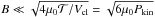 .
.
We note, however, that the density of the absorbing and infalling gas may be somewhat lower than the volume-average clump density.
Acknowledgments
I express my gratitude to the anonymous referee for his/her constructive comments and suggestions on the original manuscript. I wish to thank the staff at the APEX telescope for performing the service-mode observations presented in this paper. I would also like to thank the people who maintain the CDMS and JPL molecular spectroscopy databases, and the Splatalogue Database for Astronomical Spectroscopy. The Academy of Finland is acknowledged for the financial support through grant 132291. This research has made use of NASA’s Astrophysics Data System and the NASA/IPAC Infrared Science Archive, which is operated by the JPL, California Institute of Technology, under contract with the NASA.
References
- Albertsson, T., Semenov, D. A., & Henning, T. 2011, ApJ, submitted [arXiv:1110.2644] [Google Scholar]
- André, P., Men’shchikov, A., Bontemps, S., et al. 2010, A&A, 518, L102 [NASA ADS] [CrossRef] [EDP Sciences] [Google Scholar]
- Bachiller, R., & Perez Gutierrez, M. 1997, ApJ, 487, L93 [NASA ADS] [CrossRef] [Google Scholar]
- Ballesteros-Paredes, J. 2006, MNRAS, 372, 443 [NASA ADS] [CrossRef] [Google Scholar]
- Ballesteros-Paredes, J., Vázquez-Semadeni, E., & Scalo, J. 1999, ApJ, 515, 286 [NASA ADS] [CrossRef] [Google Scholar]
- Ballesteros-Paredes, J., Hartmann, L. W., Vázquez-Semadeni, E., et al. 2011, MNRAS, 411, 65 [NASA ADS] [CrossRef] [Google Scholar]
- Bastien, P. 1983, A&A, 119, 109 [NASA ADS] [Google Scholar]
- Belitsky, V., Lapkin, I., Vassilev, V., et al. 2007, in Proc. joint 32nd International Conference on Infrared Millimeter Waves and 15th International Conference on Terahertz Electronics, September 3–7, 2007 (Cardiff, Wales, UK: City Hall), 326 [Google Scholar]
- Beltrán, M. T., Brand, J., Cesaroni, R., et al. 2006, A&A, 447, 221 [NASA ADS] [CrossRef] [EDP Sciences] [MathSciNet] [Google Scholar]
- Beltrán, M. T., Cesaroni, R., Neri, R., & Codella, C. 2011, A&A, 525, A151 [NASA ADS] [CrossRef] [EDP Sciences] [Google Scholar]
- Bertoldi, F., & McKee, C. F. 1992, ApJ, 395, 140 (BM92) [NASA ADS] [CrossRef] [Google Scholar]
- Beuther, H., & Sridharan, T. K. 2007, ApJ, 668, 348 [NASA ADS] [CrossRef] [Google Scholar]
- Beuther, H., Schilke, P., Menten, K. M., et al. 2002, ApJ, 566, 945 [NASA ADS] [CrossRef] [Google Scholar]
- Beuther, H., Kainulainen, J., Henning, T., et al. 2011, A&A, 533, A17 [NASA ADS] [CrossRef] [EDP Sciences] [Google Scholar]
- Bonazzola, S., Heyvaerts, J., Falgarone, E., et al. 1987, A&A, 172, 293 [NASA ADS] [Google Scholar]
- Bonnell, I. A., & Bate, M. R. 2006, MNRAS, 370, 488 [NASA ADS] [CrossRef] [Google Scholar]
- Brand, J., & Blitz, L. 1993, A&A, 275, 67 [NASA ADS] [Google Scholar]
- Bronfman, L., Cohen, R. S., Alvarez, H., et al. 1988, ApJ, 324, 248 [NASA ADS] [CrossRef] [Google Scholar]
- Carey, S. J., Clark, F. O., Egan, M. P., et al. 1998, ApJ, 508, 721 [NASA ADS] [CrossRef] [Google Scholar]
- Carey, S. J., Feldman, P. A., Redman, R. O., et al. 2000, ApJ, 543, L157 [NASA ADS] [CrossRef] [Google Scholar]
- Cazzoli, G., Puzzarini, C., & Lapinov, A. V. 2004, ApJ, 611, 615 [NASA ADS] [CrossRef] [Google Scholar]
- Chandrasekhar, S. 1951, Proc. R. Soc. Lond. A, 210, 26 [Google Scholar]
- Chandrasekhar, S., & Fermi, E. 1953, ApJ, 118, 116 [NASA ADS] [CrossRef] [MathSciNet] [Google Scholar]
- Charnley, S. B., Ehrenfreund, P., Millar, T. J., et al. 2004, MNRAS, 347, 157 [NASA ADS] [CrossRef] [Google Scholar]
- Chen, X., Shen, Z.-Q., Li, J.-J., et al. 2010, ApJ, 710, 150 [NASA ADS] [CrossRef] [Google Scholar]
- Chen, H.-R., Liu, S.-Y., Su, Y.-N., & Wang, M.-Y. 2011, ApJ, 743, 196 [NASA ADS] [CrossRef] [Google Scholar]
- Curry, C. L. 2000, ApJ, 541, 831 [NASA ADS] [CrossRef] [Google Scholar]
- Davies, B., Hoare, M. G., Lumsden, S. L., et al. 2011, MNRAS, 416, 972 [NASA ADS] [CrossRef] [Google Scholar]
- Devine, K. E., Chandler, C. J., Brogan, C., et al. 2011, ApJ, 733, 44 [NASA ADS] [CrossRef] [Google Scholar]
- Egan, M. P., Shipman, R. F., Price, S. D., et al. 1998, ApJ, 494, L199 [NASA ADS] [CrossRef] [Google Scholar]
- Evans, N. J., II 1999, ARA&A, 37, 311 [NASA ADS] [CrossRef] [Google Scholar]
- Fiege, J. D., & Pudritz, R. E. 2000a, MNRAS, 311, 85 [NASA ADS] [CrossRef] [Google Scholar]
- Fiege, J. D., & Pudritz, R. E. 2000b, MNRAS, 311, 105 [NASA ADS] [CrossRef] [Google Scholar]
- Fiege, J. D., Johnstone, D., Redman, R. O., & Feldman, P. A. 2004, ApJ, 616, 925 [NASA ADS] [CrossRef] [Google Scholar]
- Field, G. B., Blackman, E. G., & Keto, E. R. 2011, MNRAS, 416, 710 [NASA ADS] [Google Scholar]
- Fontani, F., Beltrán, M. T., Brand, J., et al. 2005, A&A, 432, 921 [NASA ADS] [CrossRef] [EDP Sciences] [Google Scholar]
- Fontani, F., Caselli, P., Crapsi, A., et al. 2006, A&A, 460, 709 [NASA ADS] [CrossRef] [EDP Sciences] [Google Scholar]
- Frerking, M. A., Langer, W. D., & Wilson, R. W. 1982, ApJ, 262, 590 [NASA ADS] [CrossRef] [Google Scholar]
- Fuller, G. A., & Myers, P. C. 1992, ApJ, 384, 523 [NASA ADS] [CrossRef] [Google Scholar]
- Galli, D., Walmsley, M., & Gonçalves, J. 2002, A&A, 394, 275 [NASA ADS] [CrossRef] [EDP Sciences] [Google Scholar]
- Garrod, R. T., & Herbst, E. 2006, A&A, 457, 927 [NASA ADS] [CrossRef] [EDP Sciences] [Google Scholar]
- Garrod, R. T., Weaver, S. L. W., & Herbst, E. 2008, ApJ, 682, 283 [NASA ADS] [CrossRef] [Google Scholar]
- Goldsmith, P. F., & Langer, W. D. 1999, ApJ, 517, 209 [NASA ADS] [CrossRef] [Google Scholar]
- Gómez, L., Wyrowski, F., Pillai, T., et al. 2011, A&A, 529, A161 [NASA ADS] [CrossRef] [EDP Sciences] [Google Scholar]
- Güsten, R., Nyman, L. Å., Schilke, P., et al. 2006, A&A, 454, L13 [NASA ADS] [CrossRef] [EDP Sciences] [Google Scholar]
- Hartquist, T. W., Dalgarno, A., & Oppenheimer, M. 1980, ApJ, 236, 182 [NASA ADS] [CrossRef] [Google Scholar]
- Hatchell, J., Thompson, M. A., Millar, T. J., & MacDonald, G. H. 1998, A&AS, 133, 29 [NASA ADS] [CrossRef] [EDP Sciences] [Google Scholar]
- Heitsch, F., Hartmann, L. W., Slyz, A. D., et al. 2008, ApJ, 674, 316 [NASA ADS] [CrossRef] [Google Scholar]
- Heitsch, F., Ballesteros-Paredes, J., & Hartmann, L. 2009, ApJ, 704, 1735 [NASA ADS] [CrossRef] [Google Scholar]
- Heitsch, F., Naab, T., & Walch, S. 2011, MNRAS, 415, 271 [NASA ADS] [CrossRef] [Google Scholar]
- Hennemann, M., Birkmann, S. M., Krause, O., et al. 2009, ApJ, 693, 1379 [NASA ADS] [CrossRef] [Google Scholar]
- Henning, T., Linz, H., Krause, O., et al. 2010, A&A, 518, L95 [NASA ADS] [CrossRef] [EDP Sciences] [Google Scholar]
- Hernandez, A. K., Tan, J. C., Caselli, P., et al. 2011, ApJ, 738, 11 [NASA ADS] [CrossRef] [Google Scholar]
- Hiraoka, K., Ushiama, S., Enoura, T., et al. 2006, ApJ, 643, 917 [NASA ADS] [CrossRef] [Google Scholar]
- Inutsuka, S.-I., & Miyama, S. M. 1992, ApJ, 388, 392 [NASA ADS] [CrossRef] [Google Scholar]
- Jackson, J. M., Finn, S. C., Chambers, E. T., et al. 2010, ApJ, 719, L185 [NASA ADS] [CrossRef] [Google Scholar]
- Jefferts, K. B., Penzias, A. A., & Wilson, R. W. 1973, ApJ, 179, L57 [NASA ADS] [CrossRef] [Google Scholar]
- Jiménez-Serra, I., Caselli, P., Tan, J. C., et al. 2010, MNRAS, 406, 187 [NASA ADS] [CrossRef] [Google Scholar]
- Johnstone, D., Fiege, J. D., Redman, R. O., et al. 2003, ApJ, 588, L37 [NASA ADS] [CrossRef] [Google Scholar]
- Kainulainen, J., Beuther, H., Banerjee, R., et al. 2011a, A&A, 530, A64 [NASA ADS] [CrossRef] [EDP Sciences] [Google Scholar]
- Kainulainen, J., Alves, J., Beuther, H., et al. 2011b, A&A, 536, A48 [NASA ADS] [CrossRef] [EDP Sciences] [Google Scholar]
- Kang, M., Choi, M., Bieging, J. H., et al. 2011, ApJ, 743, 198 [NASA ADS] [CrossRef] [Google Scholar]
- Kauffmann, J., & Pillai, T. 2010, ApJ, 723, L7 [NASA ADS] [CrossRef] [Google Scholar]
- Klaassen, P. D., & Wilson, C. D. 2007, ApJ, 663, 1092 [NASA ADS] [CrossRef] [Google Scholar]
- Klein, B., Philipp, S. D., Krämer, I., et al. 2006, A&A, 454, L29 [NASA ADS] [CrossRef] [EDP Sciences] [Google Scholar]
- Klessen, R. S. 2001, ApJ, 556, 837 [Google Scholar]
- Klessen, R. S., & Burkert, A. 2000, ApJS, 128, 287 [NASA ADS] [CrossRef] [Google Scholar]
- Lada, C. J., Muench, A. A., Rathborne, J., et al. 2008, ApJ, 672, 410 [NASA ADS] [CrossRef] [Google Scholar]
- Ladd, E. F., Fuller, G. A., & Deane, J. R. 1998, ApJ, 495, 871 [NASA ADS] [CrossRef] [Google Scholar]
- Leurini, S., Pillai, T., Stanke, T., et al. 2011, A&A, 533, A85 [NASA ADS] [CrossRef] [EDP Sciences] [Google Scholar]
- Lucas, R. 1976, A&A, 46, 473 [NASA ADS] [Google Scholar]
- Mangum, J. G., Plambeck, R. L., & Wootten, A. 1991, ApJ, 369, 169 [NASA ADS] [CrossRef] [Google Scholar]
- McKee, C. F., & Zweibel, E. G. 1992, ApJ, 399, 551 [NASA ADS] [CrossRef] [Google Scholar]
- McKee, C. F., & Tan, J. C. 2003, ApJ, 585, 850 [NASA ADS] [CrossRef] [MathSciNet] [Google Scholar]
- Miettinen, O., & Harju, J. 2010, A&A, 520, A102 (Paper I) [NASA ADS] [CrossRef] [EDP Sciences] [Google Scholar]
- Miettinen, O., Hennemann, M., & Linz, H. 2011, A&A, 534, A134 [NASA ADS] [CrossRef] [EDP Sciences] [Google Scholar]
- Müller, H. S. P., Schlöder, F., Stutzki, J., & Winnewisser, G. 2005, J. Mol. Struct., 742, 215 [NASA ADS] [CrossRef] [Google Scholar]
- Myers, P. C. 2009, ApJ, 700, 1609 [NASA ADS] [CrossRef] [EDP Sciences] [Google Scholar]
- Myers, P. C., Ladd, E. F., & Fuller, G. A. 1991, ApJ, 372, L95 [NASA ADS] [CrossRef] [Google Scholar]
- Myers, P. C., Mardones, D., Tafalla, M., et al. 1996, ApJ, 465, L133 [NASA ADS] [CrossRef] [Google Scholar]
- Nagasawa, M. 1987, Prog. Theor. Phys., 77, 635 [NASA ADS] [CrossRef] [Google Scholar]
- Nakajima, Y., & Hanawa, T. 1996, ApJ, 467, 321 [NASA ADS] [CrossRef] [EDP Sciences] [Google Scholar]
- Nakamura, F., Hanawa, T., & Nakano, T. 1993, PASJ, 45, 551 [NASA ADS] [Google Scholar]
- Nguyên Luong, Q., Motte, F., Hennemann, M., et al. 2011, A&A, 535, A76 [NASA ADS] [CrossRef] [EDP Sciences] [Google Scholar]
- Ostriker, J. 1964, ApJ, 140, 1056 [NASA ADS] [CrossRef] [MathSciNet] [Google Scholar]
- Pérault, M., Omont, A., Simon, G., et al. 1996, A&A, 315, L165 [Google Scholar]
- Peretto, N., & Fuller, G. A. 2009, A&A, 505, 405 [NASA ADS] [CrossRef] [EDP Sciences] [Google Scholar]
- Pickett, H. M., Poynter, I. R. L., Cohen, E. A., et al. 1998, J. Quant. Spec. Radiat. Transf., 60, 883 [Google Scholar]
- Pillai, T., Wyrowski, F., Carey, S. J., et al. 2006, A&A, 450, 569 [NASA ADS] [CrossRef] [EDP Sciences] [Google Scholar]
- Pound, M. W., & Blitz, L. 1993, ApJ, 418, 328 [NASA ADS] [CrossRef] [Google Scholar]
- Ragan, S. E., Bergin, E. A., & Gutermuth, R. A. 2009, ApJ, 698, 324 [NASA ADS] [CrossRef] [Google Scholar]
- Ragan, S. E., Bergin, E. A., & Wilner, D. 2011, ApJ, 736, 163 [NASA ADS] [CrossRef] [Google Scholar]
- Rathborne, J. M., Jackson, J. M., Chambers, E. T., et al. 2005, ApJ, 630, L181 [NASA ADS] [CrossRef] [Google Scholar]
- Rathborne, J. M., Jackson, J. M., & Simon, R. 2006, ApJ, 641, 389 [NASA ADS] [CrossRef] [Google Scholar]
- Rathborne, J. M., Jackson, J. M., Zhang, Q., & Simon, R. 2008, ApJ, 689, 1141 [NASA ADS] [CrossRef] [Google Scholar]
- Reid, M. J., Menten, K. M., Zheng, X. W., et al. 2009, ApJ, 700, 137 [NASA ADS] [CrossRef] [Google Scholar]
- Sakai, T., Sakai, N., Kamegai, K., et al. 2008, ApJ, 678, 1049 [NASA ADS] [CrossRef] [Google Scholar]
- Sakai, T., Sakai, N., Hirota, T., & Yamamoto, S. 2010, ApJ, 714, 1658 (SSH10) [NASA ADS] [CrossRef] [Google Scholar]
- Sakai, T., Sakai, N., Furuya, K., et al. 2012, ApJ, accepted [arXiv:1201.4430] [Google Scholar]
- Schilke, P., Walmsley, C. M., Pineau des Forêts, G., & Flower, D. R. 1997, A&A, 321, 293 [NASA ADS] [Google Scholar]
- Schöier, F. L., van der Tak, F. F. S., van Dishoeck, E. F., & Black, J. H. 2005, A&A, 432, 369 [NASA ADS] [CrossRef] [EDP Sciences] [Google Scholar]
- Simon, R., Jackson, J. M., Rathborne, J. M., & Chambers, E. T. 2006, ApJ, 639, 227 [NASA ADS] [CrossRef] [Google Scholar]
- Sridharan, T. K., Beuther, H., Saito, M., et al. 2005, ApJ, 634, L57 [NASA ADS] [CrossRef] [Google Scholar]
- Stodólkiewicz, J. S. 1963, Acta Astron., 13, 30 [NASA ADS] [Google Scholar]
- Tafalla, M., Santiago-García, J., Myers, P. C., et al. 2006, A&A, 455, 577 [NASA ADS] [CrossRef] [EDP Sciences] [Google Scholar]
- Teyssier, D., Hennebelle, P., & Pérault, M. 2002, A&A, 382, 624 [NASA ADS] [CrossRef] [EDP Sciences] [Google Scholar]
- Townes, C. H., & Schawlow, L. S. 1975, Microwave Spectroscopy (New York: Dover Publications, Inc.) [Google Scholar]
- Turner, B. E. 1991, ApJS, 76, 617 [NASA ADS] [CrossRef] [Google Scholar]
- van der Tak, F. F. S., van Dishoeck, E. F., & Caselli, P. 2000, A&A, 361, 327 [NASA ADS] [Google Scholar]
- Vassilev, V., Meledin, D., Lapkin, I., et al. 2008a, A&A, 490, 1157 [NASA ADS] [CrossRef] [EDP Sciences] [Google Scholar]
- Vassilev, V., Henke, D., Lapkin, I., et al. 2008b, IEEE Microwave and Wireless Components Letters, 18, 1, 55 [Google Scholar]
- Wang, K., Zhang, Q., Wu, Y., & Zhang, H. 2011, ApJ, 735, 64 [NASA ADS] [CrossRef] [Google Scholar]
- Whittet, D. C. B., Cook, A. M., Herbst, E., et al. 2011, ApJ, 742, 28 [NASA ADS] [CrossRef] [Google Scholar]
- Williams, J. P., de Geus, E. J., & Blitz, L., 1994, ApJ, 428, 693 [NASA ADS] [CrossRef] [Google Scholar]
- Wilson, T. L., & Rood, R. 1994, ARA&A, 32, 191 [NASA ADS] [CrossRef] [Google Scholar]
- Wirström, E. S., Geppert, W. D., Hjalmarson, Å., et al. 2011, A&A, 533, A24 [NASA ADS] [CrossRef] [EDP Sciences] [Google Scholar]
- Zapata, L. A., Palau, A., Ho, P. T. P., et al. 2008, A&A, 479, L25 [NASA ADS] [CrossRef] [EDP Sciences] [Google Scholar]
- Zhang, Q., Wang, Y., Pillai, T., & Rathborne, J. 2009, ApJ, 696, 268 [NASA ADS] [CrossRef] [Google Scholar]
- Zhang, S. B., Yang, J., Xu, Y., et al. 2011, ApJS, 193, 10 [NASA ADS] [CrossRef] [Google Scholar]
- Zhou, S., Evans, N. J., II, Koempe, C., & Walmsley, C. M. 1993, ApJ, 404, 232 [NASA ADS] [CrossRef] [Google Scholar]
Appendix A: Derivation of the physical and chemical properties of the cloud/clumps
This appendix details the analysis and formulae discussed in Sects. 4.1–4.4.
A.1. Kinematic distance
To calculate the cloud kinematic distance, we adopted the mean C17O(2−1) radial velocity of −26.7 km s-1. We also employed the rotation curve of Reid et al. (2009), which is based on measurements of trigonometric parallaxes and the proper motions of masers in high-mass star-forming regions. The best-fit rotation parameters of Reid et al. (2009) are (Θ0, R0) = (254 km s-1, 8.4 kpc), where R0 is the solar Galactocentric distance and Θ0 is the rotation velocity at R0. The resulting near kinematic distance, as expected to be appropriate for an IRDC seen in absorption, is d = 2.54 ± 0.66 kpc. The corresponding Galactocentric distance is about RGC ≃ 7.26 kpc. Besides being an IRDC, the Galactic latitude of G304.74,  , indeed supports the idea that it lies at the near distance, because then the cloud is ~59 pc above the Galactic plane. In the case of the far kinematic distance, which is ~7.05 kpc, it would be suspiciously high above the Galactic plane, i.e., ~162 pc. This would be more than twice the scale height of the molecular disk, z1/2 ~ 70 pc (Bronfman et al. 1988; see also Fontani et al. 2005).
A.2. Revision of clump properties presented in Paper I
The revised cloud distance was used to recalculate the distance-dependent clump parameters presented in Paper I, i.e., the clump radius (R ∝ d), mass (M ∝ d2), and volume-averaged H2 number density (⟨n(H2)⟩ ∝ M/R3 ∝ d-1) (see Eqs. (6)–(8) in Paper I). We previously assumed a uniform dust temperature of Tdust = 15 K for all the other sources except IRAS 13037 and IRAS 13039, for which we used the value ≃22 K derived from their spectral energy distributions (SEDs; see Fig. 5 of Paper I). Here, we adopt these same temperature values but the assumed 15 K temperature is now assumed to have a ±5 K uncertainty. This is expected to be a reasonable choice, because previous molecular-line observations of clumps within IRDCs have shown the typical gas kinetic temperature to lie in the range Tkin ≈ 10 − 20 K (Carey et al. 1998; Teyssier et al. 2002; Sridharan et al. 2005; Pillai et al. 2006; Sakai et al. 2008; Zhang et al. 2011; Devine et al. 2011; Ragan et al. 2011). Moreover, at high densities of n(H2) ≳ 3 × 104 cm-3, where collisional coupling between the gas and dust becomes efficient, the gas and dust temperatures are expected to be similar (e.g., Galli et al. 2002). For comparison, Nguyên Luong et al. (2011) derived a mean dust temperature of ~14.5 K for the clumps/cores in the filamentary IRDC G035.39-00.33. To estimate the errors in R, M, and ⟨ n(H2) ⟩ , we took into account the temperature uncertainty, and the distance error of ± 0.66 kpc. The ± 5-K temperature error was also used to estimate the uncertainty in the H2 column density.
Spectroscopic properties of the observed transitions.
A.3. Molecular column densities and fractional abundances
The spectral line intensity can be expressed as the main-beam brightness temperature, which is given by ![Mathematical equation: \appendix \setcounter{section}{1} \begin{equation} T_{\rm MB}=\frac{h\nu}{k_{\rm B}}\left[F(T_{\rm ex})-F(T_{\rm bg})\right]\left(1-{\rm e}^{-\tau_{\nu}} \right) , \label{eq01} \end{equation}](/articles/aa/full_html/2012/04/aa18552-11/aa18552-11-eq653.png) (A.1)where h is the Planck constant, kB is the Boltzmann constant, Tex is the line excitation temperature, Tbg is the background temperature (taken to be the cosmic background radiation temperature of 2.725 K), τν is the line optical thickness, and the function F(T) is identical to the (average) photon occupation number
(A.1)where h is the Planck constant, kB is the Boltzmann constant, Tex is the line excitation temperature, Tbg is the background temperature (taken to be the cosmic background radiation temperature of 2.725 K), τν is the line optical thickness, and the function F(T) is identical to the (average) photon occupation number  (A.2)We note that the often used Rayleigh-Jeans equivalent temperature is given by J(T) = hν/kB × F(T). From Eq. (A.1), we can solve for the peak optical thickness
 ![Mathematical equation: \appendix \setcounter{section}{1} \begin{equation} \tau_0=-\ln \left \{ 1-\frac{T_{\rm MB}}{\frac{h\nu}{k_{\rm B}}\left[F(T_{\rm ex})-F(T_{\rm bg})\right]} \right \} \cdot \label{eq02} \end{equation}](/articles/aa/full_html/2012/04/aa18552-11/aa18552-11-eq662.png) (A.3)Equation (A.3) was used to estimate the value of τ0 for the lines used in the column-density calculations (see Col. (7) of Table 3). The assumptions made concerning the value of Tex are described below.
(A.3)Equation (A.3) was used to estimate the value of τ0 for the lines used in the column-density calculations (see Col. (7) of Table 3). The assumptions made concerning the value of Tex are described below.
The beam-averaged column densities, N(mol), of C17O, SiO, CH3OH, and DCN were calculated under the assumption of local thermodynamic equilibrium (LTE), and assuming optically thin emission. The latter assumption seems to be valid for our lines. In this case, N(mol) is directly proportional to the integrated line intensity as
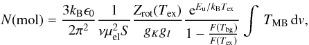 (A.4)where ϵ0 is the vacuum permittivity, μel is the permanent electric dipole moment, S is the line strength, Zrot is the rotational partition function, gK is the K-level degeneracy, gI is the reduced nuclear spin degeneracy (see, e.g., Turner 1991), and Eu is the energy of the upper-transition state. We note that in the derivation of Eq. (A.4), the electric dipole moment matrix element is defined to be
  , where gu = 2J + 1 is the rotational degeneracy of the upper state (Townes & Schawlow 1975). For linear molecules, we note that gK = gI = 1 for all levels, whereas for A-type CH3OH, gK = 1 and gI = 2, and for E-type CH3OH, gK = 2 and gI = 1 (Turner 1991). We derived the CH3OH column densities from the integrated intensity of both the CH3OH(50,5 − 40,4)-A+ and CH3OH(5 − 1,5 − 4 − 1,4)-E lines, and the results were found to be comparable to each other. In this paper, we only give the N(CH3OH) values derived from the above A+-transition. We note that we detected too few lines to employ the population diagram analysis to derive the rotational temperature and column density of CH3OH (Goldsmith & Langer 1999).
For the linear molecules C17O, SiO, and DCN, we approximated the partition function as
 (A.5)where B is the rotational constant. The above expression is appropriate for heteropolar molecules at the high temperature limit (hB/kBTex ≪ 1). The partition function of methanol, which is a slightly asymmetric rotor with one internal rotor and A- and E-symmetry states, was calculated as
  (A.6)where A, B, and C are the rotational constants (Turner 1991). The spectroscopic properties of the observed molecules/transitions are given in Table A.1
The unknown parameter in the above optical-thickness and column-density calculations is the excitation temperature, Tex. In the case of C17O, we assumed that the line is thermalised at the clump temperature, and adopted the value Tex = 15 ± 5 K for all the clumps except the IRAS sources 13037 and 13039, for which the value Tex = 22 K was used (Appendix A.2). This is likely to be true for our clumps, because even their average H2 densities are comparable to the critical density of C17O(2 − 1) (9.5 × 103 cm-3; see Col. (2) of Table A.1). Fontani et al. (2005) derived the C17O rotational excitation temperature towards IRAS 13039 of 18 K, which is very close to the value we adopted. The approximate-equality Tkin ≃ Tex [C17O(2 − 1)] was derived by Miettinen et al. (2011) for a sample of clumps associated with IRDCs. For the linear rotors SiO and DCN, we assumed that Tex is in the range [5 K, Eu/kB] , whereas for CH3OH it was assumed that Tex ∈ [10 K, 2Eu/3kB] . The adopted upper Tex limits result from the turning point of the temperature-dependent part of N(mol), i.e., from the derivative
 (A.7)where it is assumed that Tex ≫ Tbg (e.g., Hatchell et al. 1998). The upper Tex limits thus derived lead to the lower limit to N(mol). We note that the Tex(CH3OH) range we used, 10–23.2 K, is comparable to the CH3OH(2k − 1k) rotational temperatures of ~ 13.4 − 24.5 K derived by SSH10 towards a sample of massive clumps within IRDCs.
We calculated the fractional abundances of the molecules by dividing the molecular column density by the H2 column density: x(mol) = N(mol)/N(H2). For this purpose, the values of N(H2) were derived from the LABOCA dust continuum map smoothed to the corresponding resolution of the line observations.
A.4. CO depletion factors
Since the clumps under investigation (or at least most of them) are presumably cold, the CO molecules should efficiently freeze out onto dust grain surfaces. To estimate the extent of this CO depletion, we calculated the CO depletion factors, fD, following the analysis presented in the paper by Fontani et al. (2006). If x(CO)can is the “canonical” (undepleted) abundance of CO, and x(CO)obs is the observed CO abundance, fD is given by  (A.8)The “canonical” CO abundance at the Galactocentric distance RGC was calculated using the relationship (Eq. (7) in Fontani et al. 2006)
 ![Mathematical equation: \appendix \setcounter{section}{1} \begin{equation} x({\rm CO})_{\rm can}=9.5\times10^{-5}{\rm e}^{1.105-0.13R_{\rm GC}[{\rm kpc}]}. \end{equation}](/articles/aa/full_html/2012/04/aa18552-11/aa18552-11-eq697.png) (A.9)We note that this relationship assumes that R0 = 8.5 kpc, whereas our RGC value was computed using R0 = 8.4 kpc. This small discrepancy is however negligible. At RGC = 8.5 kpc, the above relationship gives the standard value 9.5 × 10⁻⁵ for the abundance of the main CO isotopologue in the solar neighbourhood (Frerking et al. 1982). At the Galactocentric distance of G304.74, x(CO)can ≃ 1.1 × 10⁻⁴. To calculate the “canonical” C17O abundance we employ the oxygen-isotopic ratio (Wilson & Rood 1994)
(A.9)We note that this relationship assumes that R0 = 8.5 kpc, whereas our RGC value was computed using R0 = 8.4 kpc. This small discrepancy is however negligible. At RGC = 8.5 kpc, the above relationship gives the standard value 9.5 × 10⁻⁵ for the abundance of the main CO isotopologue in the solar neighbourhood (Frerking et al. 1982). At the Galactocentric distance of G304.74, x(CO)can ≃ 1.1 × 10⁻⁴. To calculate the “canonical” C17O abundance we employ the oxygen-isotopic ratio (Wilson & Rood 1994) ![Mathematical equation: \appendix \setcounter{section}{1} \begin{equation} \label{eq:O-ratio} \frac{[^{16}{\rm O}]}{[^{18}{\rm O}]}=58.8\times R_{\rm GC}[{\rm kpc}]+37.1 , \end{equation}](/articles/aa/full_html/2012/04/aa18552-11/aa18552-11-eq703.png) (A.10)and the ratio [18O] / [17O] = 3.52 (Frerking et al. 1982)
(A.10)and the ratio [18O] / [17O] = 3.52 (Frerking et al. 1982) ![Mathematical equation: \appendix \setcounter{section}{1} \begin{eqnarray} x({\rm C^{17}O})_{\rm can} &=& \frac{x({\rm CO})_{\rm can}}{[^{18}{\rm O}]/[^{17}{\rm O}]\times [^{16}{\rm O}]/[^{18}{\rm O}]}\nonumber \\ &=& \frac{x({\rm CO})_{\rm can}}{3.52\times(58.8\times R_{\rm GC}[{\rm kpc}]+37.1)} \cdot \end{eqnarray}](/articles/aa/full_html/2012/04/aa18552-11/aa18552-11-eq705.png) (A.11)For G304.74, we get x(C17O)can ≃ x(CO)can/1633 ≃ 6.8 × 10⁻⁸. The depletion factor fD is then calculated from fD = x(C17O)can/x(C17O)obs.
(A.11)For G304.74, we get x(C17O)can ≃ x(CO)can/1633 ≃ 6.8 × 10⁻⁸. The depletion factor fD is then calculated from fD = x(C17O)can/x(C17O)obs.
All Tables
Molecular column densities, fractional abundances with respect to H2, and CO depletion factors (fD).
The clump virial masses and virial parameters, and the estimated external pressure required to bring the clump into virial equilibrium.
All Figures
|
Fig. 1 LABOCA 870-μm image of the IRDC G304.74. The image is shown with linear scaling, and the colour bar indicates the flux density in units of Jy beam-1. The rms level is 0.03 Jy beam-1 (1σ). The first contour and the separation between contours is 3σ. The green plus signs show the submm peak positions, which were used as the line-observation target positions in the present study. The white circles indicate the nominal catalogue positions of the MSX 8-μm sources. The 1-pc scale bar and the effective LABOCA beam HPBW (~20″) are shown in the bottom left (modified from Paper I). |
| In the text | |
|
Fig. 2 Smoothed C17O(2−1) spectra. Overlaid on the spectra are the hf-structure fits. The relative velocities of individual hf components are indicated by vertical lines under the spectra. |
| In the text | |
|
Fig. 3 Smoothed 13CO(2−1) spectra overlaid with hf-structure fits. The relative velocities of individual hf components are indicated by vertical lines under the spectra. The red vertical line shows the systemic velocity derived from C17O(2−1). |
| In the text | |
|
Fig. 4 Smoothed SiO(5−4) spectra. The line was detected only towards SMM 3 (overlaid with a Gaussian fit). Note that the spectrum towards SMM 3 is shown with a wider velocity range for reasons of clarity. |
| In the text | |
|
Fig. 5 Smoothed CH3OH(5k − 4k) spectra with Gaussian fits overlaid. In the spectrum towards SMM 2, the CH3OH(54,1 − 44,0)-A+ and CH3OH(54,2 − 44,1)-A− transitions are blended. Note that the velocity range shown is different for SMM 2 for reasons of clarity. |
| In the text | |
|
Fig. 6 The smoothed DCN(3 − 2) spectrum towards SMM 3. The line is overlaid with a hf-structure fit, and the vertical lines show the relative velocities of individual hf components. |
| In the text | |
|
Fig. 7 Relation between mass and effective radius for the clumps in G304.74. The solid line shows the least squares fit to the data, i.e., log (M) ≈ 3.1 + 2.8log (R). The dotted line represents the mass-radius threshold for massive-star formation proposed by Kauffmann & Pillai (2010), i.e., M(R) = 870 M⊙ × (R/pc)1.33. |
| In the text | |
|
Fig. 8 Left: the FWHM linewidth of C17O(2 − 1) versus clump effective radius. Right: the σNT/cs ratio versus clump mass. The dashed line represents the limit between subsonic and supersonic non-thermal motions, i.e., σNT/cs = 1. |
| In the text | |
|
Fig. 9 Relation between virial parameter and mass for the clumps in G304.74. The solid line is the least squares fit to the data, i.e., log (αvir) ≃ 1.4 − 0.7log (M). The dashed line indicates the virial-equilibrium limit of αvir = 1, and the dash-dotted line shows the limit of gravitational boundedness or αvir = 2. |
| In the text | |
Current usage metrics show cumulative count of Article Views (full-text article views including HTML views, PDF and ePub downloads, according to the available data) and Abstracts Views on Vision4Press platform.
Data correspond to usage on the plateform after 2015. The current usage metrics is available 48-96 hours after online publication and is updated daily on week days.
Initial download of the metrics may take a while.