| Issue |
A&A
Volume 540, April 2012
|
|
|---|---|---|
| Article Number | A93 | |
| Number of page(s) | 7 | |
| Section | Extragalactic astronomy | |
| DOI | https://doi.org/10.1051/0004-6361/201118364 | |
| Published online | 03 April 2012 | |
Improved distance determination to M 51 from supernovae 2011dh and 2005cs
1 Department of Optics and Quantum Electronics, University of Szeged, Dóm tér 9, 6720 Szeged, Hungary
e-mail: vinko@physx.u-szeged.hu
2 Harvard-Smithsonian Center for Astrophysics, 60 Garden St, Cambridge, MA 02138, USA
3 Department of Astronomy, University of Texas at Austin, 1 University Station C1400, Austin, TX 78712-0259, USA
4 Konkoly Observatory of the Hungarian Academy of Sciences, POB 67, 1525 Budapest, Hungary
5 Department of Physics, University of Notre Dame, 225 Nieuwland Science Hall, Notre Dame, IN 46556, USA
6 Department of Astronomy, Loránd Eötvös University, POB 32, 1518 Budapest, Hungary
Received: 30 October 2011
Accepted: 15 February 2012
Aims. The appearance of two recent supernovae, SN 2011dh and 2005cs, both in M 51, provides an opportunity to derive an improved distance to their host galaxy by combining the observations of both SNe.
Methods. We apply the Expanding Photosphere Method to get the distance to M 51 by fitting the data of these two SNe simultaneously. In order to correct for the effect of flux dilution, we use correction factors (ζ) appropriate for standard type II-P SNe atmospheres for 2005cs, but find ζ ~ 1 for the type IIb SN 2011dh, which may be due to the reduced H-content of its ejecta.
Results. The EPM analysis resulted in DM 51 = 8.4 ± 0.7 Mpc. Based on this improved distance, we also re-analyze the HST observations of the proposed progenitor of SN 2011dh. We confirm that the object detected on the pre-explosion HST-images is unlikely to be a compact stellar cluster. In addition, its derived radius (~277 R⊙) is too large for being the real (exploded) progenitor of SN 2011dh.
Conclusions. The supernova-based distance, D = 8.4 Mpc, is in good agreement with other recent distance estimates to M 51.
Key words: supernovae: individual: 2011dh / supernovae: individual: 2005cs / galaxies: individual: M 51 / galaxies: distances and redshifts
© ESO, 2012
1. Introduction
The recent discovery of supernova (SN) 2011dh (Griga et al. 2011) attracted great attention, because this was the second bright SN in the nearby galaxy M 51 within a few years, after SN 2005cs (Kloehr et al. 2005). Both objects were core-collapse SNe. SN 2005cs was classified as a peculiar, subluminous, low-velocity type II-P SN (Modjaz et al. 2005; Pastorello et al. 2006), while SN 2011dh turned out to be a rare type IIb event (Arcavi et al. 2011) with quickly decaying hydrogen lines and strengthening He features (Marion et al. 2011). Due to the proximity of the host galaxy (D ~ 8 Mpc) and the numerous pre-explosion observations available, possible progenitors of both SNe have been successfully detected. SN 2005cs is thought to be originated from a M ~ 8 M⊙ red supergiant (Maund et al. 2005; Li et al. 2006), while the proposed progenitor of SN 2011dh was a more massive yellow supergiant having M ~ 15–20 M⊙ (Maund et al. 2011; Van Dyk et al. 2011). Due to the very early discovery and the quickly responding follow-up observing campaigns, the time of explosion (actually, the moment of the initial shock breakout from the envelope of the progenitor object) has been identified within ± 1 d accuracy for both SNe.
Having two SNe at the same distance with densely sampled light curves and spectra, and accurately known explosion times offers an unprecedented chance to combine these datasets and analyze them simultaneously in order to determine an improved distance to their host galaxy. This is the aim of the present paper.
The paper is organized as follows. In Sect. 2 we outline the method we apply for the distance measurement. In Sect. 3 the photometric and spectroscopic observations are presented, while in Sect. 4 we apply the distance measurement method to these observations. Finally, we discuss the implications of the improved distance to the physical properties of the progenitor of SN 2011dh.
2. Expanding photosphere method
The expanding photosphere method (EPM) is a geometric distance measurement method that relates the angular size of the SN ejecta to its physical radius derived from the observed expansion velocity of the SN assuming homologous expansion (Kirshner & Kwan 1974; Dessart & Hillier 2005b). The angular radius of the photosphere in a homologously expanding ejecta is defined as ![\begin{equation} \theta = R_\mathrm{phot} / D = {[ R_0 + v_\mathrm{phot} \cdot (t - t_0) ]} / D, \label{eq-1} \end{equation}](/articles/aa/full_html/2012/04/aa18364-11/aa18364-11-eq12.png) (1)where D is the distance, vphot is the ejecta velocity at the position of the photosphere, R0 is the radius of the progenitor and t0 is the moment of the initial shock breakout (usually referred to as the “moment of explosion”).
(1)where D is the distance, vphot is the ejecta velocity at the position of the photosphere, R0 is the radius of the progenitor and t0 is the moment of the initial shock breakout (usually referred to as the “moment of explosion”).
In the classical form of EPM the angular radius is derived from photometric observations via the assumption that the photosphere radiates as a blackbody, but the opacity is mostly due to electron scattering, thus the blackbody photons are diluted by scattering from free electrons:  (2)where ζ(T) is the temperature-dependent correction factor describing the dilution of the radiation, fλ is the observed flux and Bλ(T) is the Planck function. Expressing the flux in magnitudes, Eq. (2) can be rewritten as
  (3)where bλ(T) is the synthetic magnitude of the blackbody flux at temperature T (Hamuy et al. 2001).
When the angular radius can be directly measured by high-resolution imaging (e.g. VLBI), Eq. (1) can be applied directly to get the distance. This is the “expanding shock front method” (ESM), which has been successfully applied for SN 1993J by Bartel et al. (2007). Very recently, the expansion of the forward shock of SN 2011dh was detected with VLBI (Martí-Vidal et al. 2011; Bietenholz et al. 2012) and EVLA (Krauss et al. 2012). Although the spatial resolution of these observations was not yet high enough to use them for distance determination, this method looks potentially applicable for SN 2011dh in the near future, when the expanding ejecta reach the necessary diameter.
In the classical EPM the distance D is inferred via least-squares fitting to the combination of Eqs. (1) and (2), after neglecting R0 (which is usually an acceptable approximation for epochs greater than ~ 5 days after shock breakout):  (4)having D and t0 as the two unknown quantities. In principle, measuring θ and vphot at two epochs may be sufficient to determine D and t0, in practice at least 5–6 observations are needed to reduce random and systematic errors. It is important to note that each observation can provide an independent estimate on D and t0, thus, the possible errors affecting the results can compensate each other, provided there are enough data that satisfy the initial assumptions.
There are several known issues with EPM that must be handled carefully before applying Eq. (4) to the observations. First, the basic assumption is that the expansion of the ejecta is spherically symmetric. It is thought to be valid in most type II SNe, however, there are cases when asymmetry is observed (Leonard et al. 2006). This is usually done via polarization measurements, as electron scattering may result in detectable net polarization in non-spherical SNe atmospheres. For SN 2005cs, one group presented R-band imaging polarimetry (Gnedin et al. 2007), reporting record-high, variable degree of linear polarization (reaching ~8%) during the early plateau phase. However, the authors do not provide details on handling the effect of instrumental polarization, and this result has not been confirmed by other studies so far, so it should be treated with caution. For SN 2011dh, there is no such observational indication for a non-spherical explosion or expansion yet. Based on the available pieces of information, we do not find compelling evidence for asymmetric ejecta geometry in either of these SNe during the plateau phase. Thus, we assume that both SNe satisfy the sphericity condition, as it was found earlier for most type II SNe.
Second, Eqs. (2) or (3) requires unreddened fluxes or magnitudes. Thus, the observed magnitudes/fluxesneed to be dereddened before applying EPM. However, as Eastman et al. (1996) and Leonard et al. (2002) pointed out, the distance is only weakly sensitive to reddening uncertainties. This is one of the advantages of EPM as a distance measurement method.
On the contrary, the results are very sensitive to the values of the photospheric velocity. Recently the issue of measuring vphot in type II-P SNe atmospheres was studied in detail by Takáts & Vinkó (2012). They showed the applicability of the spectral modeling code SYNOW (Branch et al. 2002) to assign objective and reliable vphot to the observed spectra. In this paper we use the same technique, i.e. SYNOW to calculate vphot at each observed phase.
Finally, the exact values of the correction factors ζ(T) are still debated. Eastman et al. (1996) and Dessart & Hillier (2005b) provided ζ(T) for H-rich type II-P atmospheres, but the values from the latter study are systematically (~50%) bigger than from the former one. Moreover, in He-rich (type IIb SNe) atmospheres the correction factors are much less known. We will discuss this issue in more detail below.
In the followings we exploit the opportunity of having independent datasets from two SNe in the same host galaxy M 51 (i.e. at the same distance), and the rare and fortunate circumstance that both of them have known, accurate ( ± 1 d) shock breakout date. If t0 is known independently, Eq. (4) can be rearranged into the following form:  (5)where we introduced Δt = t − t0, and now D is the only remaining unknown. Combining the data from both SNe, Eq. (5) can be used to get an improved estimate for D, which will be applied to SN 2011dh and SN 2005cs in Sect. 4. This way we expect to eliminate much of the systematic uncertainties of EPM (arising from the correlation between the parameters t0 and D) that may sometimes bias the analysis of single SNe.
3. Observations
For SN 2005cs extensive data have been published. We have collected the BVRI light curves from Pastorello et al. (2009). The spectra published in the same paper were kindly provided to us by Andrea Pastorello.
More recently, SN 2011dh was observed with many instruments, but most of them are not published at the time of writing this paper. In the followings we present some of them that we use in our analysis.
BVRI photometry of SN 2011dh.
3.1. Photometry of SN 2011dh
For SN 2011dh, ground-based photometric observations were taken from Piszkéstető Mountain Station of Konkoly Observatory, Hungary. We have used the 60/90 cm Schmidt-telescope with the attached 4096 × 4096 CCD (FoV 70 × 70 arcmin2, equipped with Bessel BVRI filters). In Table 1 we present the data for the first 18 nights, derived by PSF-photometry in IRAF1. Note that although there are numerous pre-explosion frames of M 51 available, the background at the SN site is relatively faint and smooth, thus, we did not find the application of image subtraction necessary to obtain reliable photometric information when the SN was around maximum light.
Transformation to the standard system was computed by applying the following equations:  (6)The color terms listed above were obtained from measurements of Landolt fields on photometric nights. The zero-points for each night were tied to local tertiary standard stars around M 51 collected from Pastorello et al. (2009).
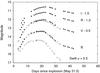 |
Fig. 1 Observed light curve of SN 2011dh. The Konkoly data are plotted with filled symbols, while Swift ubv data are denoted with open circles. Vertical shifts are applied between the data corresponding to different filters for better visibility. |
In Fig. 1 we plot and compare our measurements with the ubv data obtained by Swift/UVOT (details for the latter dataset will be given by Marion et al., in prep.). The agreement between the ground-based and space-born optical data (i.e. B and V) is excellent. We are confident that our photometry for SN 2011dh is accurate and reliable.
3.2. Spectroscopy of SN 2011dh
Optical spectra were obtained with the HET Marcario Low Resolution Spectrograph (LRS, spectral coverage 4200–10 200 Å, resolving power λ/Δλ ~ 600) at McDonald Observatory, Texas, on 6 epochs between June 6 and 22, 2011. Reduction and calibration of these data were made with standard routines in IRAF. Details will be given in Marion et al. (in prep.). The spectra are shown in Fig. 2.
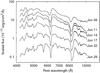 |
Fig. 2 Observed low-resolution HET spectra of SN 2011dh. Note that scales on both axes are logarithmic, and scaling factors have been applied to separate the spectra for better visibility. |
In addition, a single high-resolution spectrum were obtained with the HET High-Resolution Spectrograph (HRS, spectral coverage 4100–7800 Å, resolving power ~15 000) on June 6, 2011, in parallel with the LRS observations. No narrow features were present in the spectrum except the Na D doublet at zero velocity that are expected to be due to interstellar matter (ISM) in the Milky Way. The spectrum around these features is plotted in Fig. 3. We will use the high-resolution spectrum to constrain the interstellar reddening toward SN 2011dh in Sect. 4.
4. Analysis
In the followings we use the data presented in Sect. 3 to estimate the angular radii and photospheric velocities as a function of phase in order to perform the EPM-analysis outlined in Sect. 2.
4.1. Reddening
Fortunately, the reddening toward M 51 is low. The galactic component, due to Milky Way ISM, is estimated from the map of Schlegel et al. (1998) as E(B − V)gal = 0.035 mag. The equivalent widths of the galactic Na D features shown in Fig. 3 are consistent with this value. As seen, no significant contribution from the M 51 ISM is detected in the SN 2011dh spectrum. Therefore, E(B − V) = 0.035 mag is assumed for SN 2011dh.
For SN 2005cs we adopted a slightly higher value, E(B − V) = 0.05 mag, after Pastorello et al. (2009).
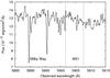 |
Fig. 3 High-resolution HET spectrum of SN 2011dh observed on June 6, 2011 (6 days after explosion). Vertical lines indicate the expected positions of the NaD doublet features in the Milky Way (dotted line) and in M 51 (continuous line). |
4.2. Photospheric velocities
In this paper we use the photospheric velocities derived from fitting SYNOW models to the observed spectra, as described in Takáts & Vinkó (2012). As it is shown in that paper, the vphot values determined this way are generally consistent (within ± 10–15%) with the velocities derived simply from the absorption minimum of the FeII λ5169 feature. However, the FeII velocities may systematically over- or underestimate the true vphot. SYNOW has the potential to resolve line blending, and thus to give a better estimate of vphot than finding individual (often blended) line minima (see Takáts & Vinkó 2012, for details).
In Table 2 the photospheric velocities, as well as the other physical parameters used for the EPM-analysis are presented.
4.3. Temperatures and angular radii
The calculation of the angular radii (Eq. (2)) needs observed fluxes and the effective temperature of the photosphere at the moments of the photometric observations. We have estimated these quantities in the following way. First, the observed magnitudes were dereddened with the E(B − V) values given in Sect. 4.1. Then, the reddening-free magnitudes were transformed into quasi-monochromatic fluxes following the calibration given by Bessell et al. (1998).
The photospheric temperatures were estimated by fitting blackbodies to the spectral energy distributions defined by the contemporaneous BVRI fluxes. Although this technique is approximate, it has been shown to produce a good estimate of the effective temperature for the application of EPM (Vinkó & Takáts 2007). Finally, both the inferred temperatures and the angular radii have been interpolated to the epochs of the spectroscopic observations. These data are summarized in Table 2.
Inferred physical parameters for EPM.
4.4. Correction factors for EPM
As mentioned in Sect. 2, the application of blackbodies to SN atmospheres requires correction factors that take into account electron scattering as well as line blending and other effects that alter the fluxes emerging from the photosphere.
As discussed in Takáts & Vinkó (2006), the angular radii of SN 2005cs were calculated by applying the EPM correction factors of Dessart & Hillier (2005a). However, the data on SN 2011dh were used without corrections, i.e. applying ζ = 1. This choice was motivated by the IIb classification of SN 2011dh. Because SN 2011dh is thought to have a He-rich atmosphere with a thin H-envelope, the number of free electrons in the ejecta should be much less than in type II-P SNe, like SN 2005cs. Since the largest contribution to the correction factors comes from the dilution of blackbody photons that are Thompson-scattered by free electrons, it is expected that the radiation of SN 2011dh should be much closer to a blackbody than that of SN 2005cs. In other words, due to the lower density of free electrons, the photosphere (i.e. the surface of last scattering) of SN 2011dh is expected to be much closer to the thermalization depth from which the blackbody photons emerge, than in SN 2005cs where the photosphere was above the thermalization depth in a H-rich atmosphere.
This qualitative picture is generally supported by the NLTE models of the ejecta of SN 1993J by Baron et al. (1995). They modeled the early spectral evolution of SN 1993J during the first 70 days with various chemical composition extending from solar He/H ratio to extreme He-rich atmospheres. For the He-rich compositions they computed substantially higher correction factors than for solar composition, although with considerable model-to-model scatter. Since these models may not be fully applicable to SN 2011dh, we did not attempt to use these correction factors at their face value, but note that they confirm the qualitative expectation that the ζ values should be higher, i.e. closer to unity in SN atmospheres having larger He/H ratio.
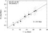 |
Fig. 4 Determination of the distance to M 51 in EPM. The slope of the fitted (solid) line gives D-1 (in Mpc-1). The dotted lines correspond to 1σ uncertainty in D, taking into account the random and the systematic errors (see text). |
4.5. Combination of SNe 2011dh and 2005cs
As it was mentioned in Sect. 1, the moment of shock breakout (t0) is accurately known for both SNe. We have adopted t0 = 2 453 549.0 JD (Pastorello et al. 2009) and t0 = 2 455 712.5 JD (Arcavi et al. 2011) for SN 2005cs and SN 2011dh, respectively.
We applied Eq. (5) for the data of both SNe (listed in Table 2) obtained during the first month, between +5 and +25 days after explosion. The motivation for using the +5 days lower limit was that the ejecta may not expand homologously at very early phases. Also, for epochs earlier than +5 days, R0 may not be negligible with respect to the vphot(t − t0) term, as we have assumed to get Eq. (5) (see Sect. 2). The restriction of selecting epochs not later than ~30 days for EPM was suggested by Dessart & Hillier (2005b). They pointed out that the basic assumptions of EPM (optically thick ejecta, less deviations from LTE condition) are valid mostly during the first month of the evolution of the ejecta. Inspecting the data in Table 2 it can be seen that θ/v changes abruptly after t ~ 22 days for both SNe, suggesting a sudden change in the ejecta physical conditions. This epoch is near the time of maximum light for SN 2011dh. From modeling the light curve of this object, Marion et al. (in prep.) pointed out that the early occurence of the peak of the light curve could be explained by a sudden drop of the Thompson-scattering opacity, possibly due to the recombination of the remaining free electrons and protons. This is analogous to the condition at the end of the plateau phase in H-rich type II-P SNe. The assumptions for EPM are certainly not valid after this phase.
Plotting of θ·v-1 vs. t − t0 gives a linear relation for which the slope equals to 1/D (see Eq. (5)). Because in this case both SNe are at the same distance, their data must fall on the same line.
Figure 4 shows that this is indeed the case. Fitting a straight line to the combined data results in an improved distance to M 51:
 The systematic error was calculated by taking into account the ± 1 d uncertainty in t0.
Our improved distance is in good agreement with the mean distance of M 51 listed in the NED2 database (D ~ 8.03 ± 0.677 Mpc), after computing the simple unweighted average of 15 individual distances. Even though these independent distance estimates represent an inhomogeneous sample in which each value may be biased by unknown systematic errors, the ~ 1σ agreement between their average and our new value is promising.
Photometry of the proposed progenitor of SN 2011dh with the Hubble Space Telescope.
5. Implications for the progenitor of SN 2011dh
The improved distance to M 51 enables us to revisit the issue of the progenitor of SN 2011dh identified on pre-explosion HST frames, immediately after discovery (Li & Filippenko 2011; Maund et al. 2011; Van Dyk et al. 2011).
We have analyzed the archival HST/ACS and WFPC2 frames independently from Maund et al. (2011) and Van Dyk et al. (2011). We followed an approach similar to Van Dyk et al. (2011) by analyzing the individual “FLT” and “C0F” frames obtained with ACS and WFPC2, respectively, by using the software packages Dolphot3 and HSTphot4 (Dolphin 2000). We have applied PSF-photometry using pre-computed PSFs, built-in corrections for charge transfer efficiency (CTE) losses and the final magnitudes were transformed into the standard Johnson-Cousins system for the broad-band filters F336W, F435W, F555W and F814W. These data are collected in Table 3 (the data in the narrow-band F658N filter are in the flight-system). Fluxes and absolute magnitudes are also presented after dereddening with E(B − V) = 0.035 mag (Sect. 4.1), using the magnitude-flux conversion by Bessell et al. (1998) and applying the distance modulus μ0 = 29.62 mag corresponding to D = 8.4 Mpc (Sect. 4.5). The uncertainties of the absolute magnitudes reflect the errors of the photometry and the random plus systematic uncertainty of the distance added in quadratures. Generally, these results are in between the values presented by Maund et al. (2011) and Van Dyk et al. (2011), and agree within 1σ uncertainty except for the F336W filter, where our magnitude is fainter by ~0.5 mag (~2σ) than that given by Maund et al. (2011) and Van Dyk et al. (2011). Given the inferior spatial resolution of the WFPC2 frames, the faintness of the source and the issue of the proper source identification on the WFPC2 images in this crowded region, the F336W magnitude in Table 3 may only be an upper limit.
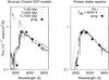 |
Fig. 5 SED of the proposed progenitor (filled circles) and SSP models with cluster ages of 60 Myr, 600 Myr and 1 Gyr (left), and an F8 supergiant model together with a T = 6000 K blackbody (right). The SED of the 60 Myr-old cluster that may contain a M > 8 M⊙ star is clearly incompatible with the measured fluxes. The older clusters that fit the data better are too old to support the presence of such a massive progenitor. |
In Fig. 5 left panel, we plot the dereddened quasi-monochromatic flux distribution together with model SEDs of Simple Stellar Populations (SSPs) by Bruzual & Charlot (2003), assuming cluster ages of 60 Myr, 600 Myr and 1 Gyr, respectively. This figure illustrates the conclusion first drawn by Maund et al. (2011), that the SED of the proposed progenitor is too red to be compatible with a young stellar cluster hosting a sufficiently massive star that can become a core-collapse SN. The oldest cluster that may be able to produce a core-collapse SN (Mprog ~ 8 M⊙) has the age of ~ 60 Myr (see e.g. Fig. 19 in Vinkó et al. 2009). Figure 5 clearly shows that the 60 Myr-old cluster SED is incompatible with the observed flux distribution. Those cluster SEDs that are consistent with the observations are at least an order of magnitude older, containing only less massive stars.
Strictly speaking, the above argument is valid only for coeval cluster stars, i.e. when all cluster members were born by an initial starburst. There is a less likely, but not unrealistic scenario, in which massive stars are formed in an active star-forming region, and a nearby compact cluster captures them. There is observational evidence that young massive clusters can capture field stars (e.g. Sandage-96 in NGC 2404, see Vinkó et al. 2009), although this process should occur very (maybe too) fast in order to explain the presence of a M > 8 M⊙ star in a t ≥ 600 Myr-old cluster.
The right panel of Fig. 5 shows the good agreement between the observed progenitor fluxes and the flux spectrum of an F8-type supergiant having Teff = 6000 K (Maund et al. 2011; Van Dyk et al. 2011). Integrating the observed SED, and adopting Teff = 6000 K and D = 8.4 ± 0.7 Mpc, the radius of the proposed progenitor turns out to be Rprog = 1.93( ± 0.16) × 1013 cm (277 ± 23 R⊙). This is very close to the result of Van Dyk et al. (2011), who derived Rprog ~ 290 R⊙ from the same data, although they adopted a slightly lower distance to M 51 (D ~ 7.6 Mpc).
As recently noted by Arcavi et al. (2011), Soderberg et al. (2011) and Van Dyk et al. (2011), the observed early optical-, radio- and X-ray observations of SN 2011dh are in sharp contrast with such a large progenitor radius. All these pieces of evidence point consistently toward a compact progenitor, Rprog ~ 1011 cm. Indeed, as discussed by Marion et al. (in prep.), modeling the bolometric light curve of SN 2011dh during the first 30 days after explosion (extending to post-maximum epochs) gives strong support to the compact progenitor hypothesis. Marion et al. (in prep.) present an upper limit for the progenitor radius as Rprog ≲ 2 × 1011 cm, in good agreement with Arcavi et al. (2011) and Soderberg et al. (2011). The radius of the observed object (R ~ 277 R⊙) derived above definitely rules out that this object was the progenitor that exploded. It remains the subject of further studies whether such an extended, yellow supergiant could be a member of a binary system containing also a hot, compact primary star, which seems to be currently the most probable configuration for the progenitor of SN 2011dh, or other hypotheses, e.g a massive star captured by a compact stellar cluster outlined above, are necessary to resolve this issue. Further observations of the SN during the nebular phase are also essential in this respect.
6. Summary
Based on the results above we draw the following conclusions:
-
We presented new photometric and spectroscopic observations of the type IIb SN 2011dh.
-
Combining these data with those of the type II-P SN 2005cs, we derived an improved distance of D = 8.4 ± 0.7 Mpc to M 51 by applying the expanding photosphere method.
-
Using the updated distance, we reanalyzed archival HST observations of the proposed progenitor of SN 2011dh. It is confirmed that the object detected at the SN position is an F8-type yellow supergiant, and it is unlikely to be the exploded progenitor.
Acknowledgments
We express our thanks to the anonymous referee for the thorough reading of the manuscript, and the useful comments that helped us improving the paper. This project has been supported by Hungarian OTKA grant K76816, and by the European Union together with the European Social Fund through the TÁMOP 4.2.2/B-10/1-2010-0012 grant. The CfA Supernova Program is supported by NSF Grant AST 09-07903. J.C.W.’s supernova group at UT Austin is supported by NSF Grant AST 11-09801. A.P. has been supported by the ESA grant PECS 98073 and by the János Bolyai Research Scholarship of the Hungarian Academy of Sciences. K.S. and K.V. acknowledge support from the the “Lendület” Program of the Hungarian Academy of Sciences and Hungarian OTKA Grant K-081421. Thanks are also due to the staff of McDonald and Konkoly Observatories for the prompt scheduling and helpful assistance during the time-critical ToO observations. The SIMBAD database at CDS, the NASA ADS and NED databases have been used to access data and references. The availability of these services is gratefully acknowledged.
References
- Arcavi, I., Gal-Yam, A., Yaron, O., et al. 2011, ApJ, 742, L18 [NASA ADS] [CrossRef] [Google Scholar]
- Baron, E., Hauschildt, P. H., Branch, D., et al. 1995, ApJ, 441, 170 [NASA ADS] [CrossRef] [Google Scholar]
- Bartel, N., Bietenholz, M. F., Rupen, M. P., & Dwarkadas, V. V. 2007, ApJ, 668, 924 [NASA ADS] [CrossRef] [Google Scholar]
- Bessell, M. S., Castelli, F., & Plez, B. 1998, A&A, 333, 231 [NASA ADS] [Google Scholar]
- Bietenholz, M. F., Brunthaler, A., Soderberg, A. M., et al. 2012, ApJ, submitted [arXiv:1201.0771] [Google Scholar]
- Branch, D., Benetti, S., Kasen, D., et al. 2002, ApJ, 566, 1005 [NASA ADS] [CrossRef] [Google Scholar]
- Bruzual, G., & Charlot, S. 2003, MNRAS, 344, 1000 [NASA ADS] [CrossRef] [Google Scholar]
- Dessart, L., & Hillier, D. J., 2005a, A&A, 437, 667 [NASA ADS] [CrossRef] [EDP Sciences] [Google Scholar]
- Dessart, L., & Hillier, D. J., 2005b, A&A, 439, 671 [NASA ADS] [CrossRef] [EDP Sciences] [Google Scholar]
- Dessart, L., Blondin, S., Brown, P. J., et al. 2008, ApJ, 675, 644 [NASA ADS] [CrossRef] [Google Scholar]
- Dolphin, A. E. 2000, PASP, 112, 1383 [NASA ADS] [CrossRef] [Google Scholar]
- Eastman, R. G., Schmidt, B. P., & Kirshner, R. 1996, ApJ, 466, 911 [NASA ADS] [CrossRef] [Google Scholar]
- Gnedin, Y. N., Larionov, V. M., Konstantinova, T. S., & Kopatskaya, E. N. 2007, AstL, 33, 736 [Google Scholar]
- Griga, T., Marulla, A., Grenier, A., et al. 2011, Central Bureau Electronic Telegrams, 2736, 1 [NASA ADS] [Google Scholar]
- Hamuy, M., Pinto, P. A., Maza, J., et al. 2001, ApJ, 558, 615 [NASA ADS] [CrossRef] [Google Scholar]
- Kirshner, R. P., & Kwan, J., 1974 ApJ, 193, 27 [NASA ADS] [CrossRef] [Google Scholar]
- Kloehr, W., Muendlein, R., Li, W., Yamaoka, H., & Itagaki, K. 2005, IAU Circ., 8553, 1 [NASA ADS] [Google Scholar]
- Krauss, M. I., Soderberg, A. M., Chomiuk, L., et al. 2012, ApJL, submitted [arXiv:1201.0770] [Google Scholar]
- Leonard, D. C., Filippenko, A. V., Gates, E. L., et al. 2002, PASP, 114, 35 [NASA ADS] [CrossRef] [Google Scholar]
- Leonard, D. C., Filippenko, A. V., Ganeshalingam, M., et al. 2006, Nature, 440, 505 [NASA ADS] [CrossRef] [PubMed] [Google Scholar]
- Li, W., & Filippenko, A. V. 2011, The Astronomer’s Telegram, 3399, 1 [NASA ADS] [Google Scholar]
- Li, W., Van Dyk, S. D., Filippenko, A. V., et al. 2006, ApJ, 641, 1060 [NASA ADS] [CrossRef] [Google Scholar]
- Marion, G. H., Kirshner, R., Wheeler, J. C., et al. 2011, The Astronomer’s Telegram, 3435, 1 [NASA ADS] [Google Scholar]
- Martí-Vidal, I., Tudose, V., Paragi, Z., et al. 2011, A&A, 535, L10 [NASA ADS] [CrossRef] [EDP Sciences] [Google Scholar]
- Maund, J. R., Smartt, S. J., & Danziger, I. J. 2005, MNRAS, 364, L33 [NASA ADS] [CrossRef] [Google Scholar]
- Maund, J. R., Fraser, M., Ergon, M., et al. 2011, ApJ, 739, L37 [NASA ADS] [CrossRef] [Google Scholar]
- Modjaz, M., Kirshner, R., Challis, P., & Hutchins, R. 2005, Central Bureau Electronic Telegrams, 174, 1 [NASA ADS] [Google Scholar]
- Pastorello, A., Sauer, D., Taubenberger, S., et al. 2006, MNRAS, 370, 1752 [NASA ADS] [CrossRef] [Google Scholar]
- Pastorello, A., Valenti, S., Zampieri, L., et al., 2009, MNRAS, 394, 2266 [NASA ADS] [CrossRef] [Google Scholar]
- Schlegel, D. J., Finkbeiner, D. P., & Davis, M. 1998, ApJ, 500, 525 [NASA ADS] [CrossRef] [Google Scholar]
- Soderberg, A. M., Margutti, R., Zauderer, B. A., et al. 2011, ApJ, submitted [arXiv:1107.1876] [Google Scholar]
- Takáts, K., & Vinkó, J. 2006, MNRAS, 372, 1735 [NASA ADS] [CrossRef] [Google Scholar]
- Takáts, K., & Vinkó, J. 2012, MNRAS, 419, 2783 [NASA ADS] [CrossRef] [Google Scholar]
- Van Dyk, S. D., Li, W., Cenko, S. B., et al. 2011, ApJ, 741, L28 [NASA ADS] [CrossRef] [Google Scholar]
- Vinkó, J., & Takáts, K. 2007, Supernova 1987A: 20 Years After: Supernovae and Gamma-Ray Bursters, ed. S.Immler, K. Weiler, & R. McCray (Melville, New York: American Institute of Physics), AIP Conf. Proc., 937, 394 [Google Scholar]
- Vinkó, J., Sárneczky, K., Balog, Z., et al. 2009, ApJ, 695, 619 [NASA ADS] [CrossRef] [Google Scholar]
All Tables
Photometry of the proposed progenitor of SN 2011dh with the Hubble Space Telescope.
All Figures
|
Fig. 1 Observed light curve of SN 2011dh. The Konkoly data are plotted with filled symbols, while Swift ubv data are denoted with open circles. Vertical shifts are applied between the data corresponding to different filters for better visibility. |
| In the text | |
|
Fig. 2 Observed low-resolution HET spectra of SN 2011dh. Note that scales on both axes are logarithmic, and scaling factors have been applied to separate the spectra for better visibility. |
| In the text | |
|
Fig. 3 High-resolution HET spectrum of SN 2011dh observed on June 6, 2011 (6 days after explosion). Vertical lines indicate the expected positions of the NaD doublet features in the Milky Way (dotted line) and in M 51 (continuous line). |
| In the text | |
|
Fig. 4 Determination of the distance to M 51 in EPM. The slope of the fitted (solid) line gives D-1 (in Mpc-1). The dotted lines correspond to 1σ uncertainty in D, taking into account the random and the systematic errors (see text). |
| In the text | |
|
Fig. 5 SED of the proposed progenitor (filled circles) and SSP models with cluster ages of 60 Myr, 600 Myr and 1 Gyr (left), and an F8 supergiant model together with a T = 6000 K blackbody (right). The SED of the 60 Myr-old cluster that may contain a M > 8 M⊙ star is clearly incompatible with the measured fluxes. The older clusters that fit the data better are too old to support the presence of such a massive progenitor. |
| In the text | |
Current usage metrics show cumulative count of Article Views (full-text article views including HTML views, PDF and ePub downloads, according to the available data) and Abstracts Views on Vision4Press platform.
Data correspond to usage on the plateform after 2015. The current usage metrics is available 48-96 hours after online publication and is updated daily on week days.
Initial download of the metrics may take a while.