© ESO, 2012

1. Introduction

The statistics of nonlinear processes in the universe often shows powerlaw-like distributions, most conspicously in energetic dynamic phenomena in astrophysics (e.g., solar and stellar flares, pulsar glitches, auroral substorms) and in catastrophic events in geophysics (e.g., earthquakes, landslides, or forest fires). The most widely known example is the distribution of earthquake magnitudes, which has a powerlaw slope of α ≈ 2.0 for the differential frequency distribution (Turcotte 1999), the so-called Gutenberg-Richter (1954) law. Bak et al. (1987, 1988) introduced the theoretical concept of self-organized criticality (SOC), which has been initially applied to sandpile avalanches at a critical angle of repose, and has been generalized to nonlinear dissipative systems that are driven in a critical state. Comprehensive reviews on this subject can be found for applications in geophysics (Turcotte 1999), solar physics (Charbonneau et al. 2001), and astrophysics (Aschwanden 2011).

Hallmarks of SOC systems are the scale-free powerlaw distributions of various event parameters, such as the peak energy dissipation rate P, the total energy E, or the time duration T of events. While the powerlaw shape of the distribution function can be explained by the statistics of nonlinear processes that have an exponential growth phase and saturate after a random time interval (e.g., Willis & Yule 1922; Fermi 1949; Rosner & Vaiana 1978; Aschwanden et al. 1998; Aschwanden 2004, 2011), no general theoretical model has been developed that predicts the numerical value of the powerlaw slope of SOC parameter distributions. Simple analytical models that characterize the nonlinear growth phase with an exponential growth time τ_G and the random distribution of risetimes with an average value of t_S, predict a powerlaw slope of α_P = 1 + t_S/τ_G for the energy dissipation rate (e.g., Rosner & Vaiana 1978; Aschwanden et al. 1998), but cellular automaton simulations suggest a much more intermittent energy release process than the idealized case of an avalanche with a single growth and decay phase. An alternative theoretical explanation for a slope α_E = 3/2 was put forward by a dimensional argument (Litvinenko 1998a), which can be derived from the definition of the kinetic energy of convective flows, but this model entails a specific physical mechanism that has not universal validity for SOC systems.

In this Paper we propose a more general concept where the powerlaw slope of the occurrence frequency distribution of SOC parameters depends on the fractal geometry of the energy dissipation domain. We aim for a universal statistical model of nonlinear energy dissipation processes that is independent of any particular physical mechanism. The fractal structure of self-organized processes has been stressed prominently from beginning (Bak et al. 1987, 1988; Bak & Chen 1989), but no quantitative theory has been put forward that links the fractal geometry to the size distribution of SOC events. Fractals have been studied independently (e.g., Mandelbrot 1977, 1983, 1985), while the fractal geometry of SOC avalanches was postulated (e.g., see textbooks of Bak 1996; Sornette 2004; Aschwanden 2011), but no general self-consistent model has been attempted.

This paper presents an analytical theory that derives a theoretical framework to quantitatively link the concept of fractal dimensions to the occurrence frequency distributions of SOC avalanche events (Sect. 2), tests of the analytical theory with numerical simulations of cellular automaton models in three Euclidean dimensions (Sect. 3), a comparison and application to solar flares (Sect. 4), and a summary of the model assumptions and conclusions (Sect. 5).

2. Theory

We derive in this section a general model of the statistics of SOC processes, but make use of a specific example of a SOC avalanche that is numerically simulated with a cellular automaton code and described in more detail in Sect. 3, to illustrate and validate our theoretical derivation.

2.1. Diffusive random walk in cellular automaton avalanches

An avalanche in a cellular automaton model propagates via nearest-neighbor interactions in random directions, wherever an unstable node is found. The state of self-organized criticality ensures that the entire system is close to the instability threshold, and thus every direction of instability propagation is equally likely once a starting location is triggered (if the re-distribution rule is defined to be isotropic). We can therefore model the propagation of unstable nodes with a random walk in a S-dimensional space, which has the characteristics of a diffusion process and propagates in the statistical average a distance x(t) that depends on the time t as, $\mathit{x}\mathrm{\left(}\mathit{t}\mathrm{\right)}\mathrm{\propto }{\mathit{t}}^{\mathrm{1}\mathit{/}\mathrm{2}}\mathit{.}$(1)As a plausibility test we check this first assumption with an example of a numerical simulation of a cellular automaton model that is described in more detail in Sect. 3. The simulated avalanche shown in Fig. 1 lasts for a duration of 712 time steps and we show snapshots of the energy dissipation rate de/dt in Fig. 1. The complete time evolution of the energy dissipation rate de(t)/dt, the total energy e(t), the fractal dimension D₂(t), and radius of the avalanche area r(t) as a function of time is shown in Fig. 3. A movie of the avalanche that shows the time evolution for all 712 time steps is included in the electronic supplementary data of this journal. The movie illustrates also that the instantaneous propagation direction of the avalanche is nearly isotropic, as we assumed here, regardless of the prior evolution in the neighborhood of the instantaneous energy release. Apparently, many of the grid points that have already been touched by the avalanche previously are still in a meta-stable state near the critical threshold that enables next-neighbor interactions.

We calculate the total time-integrated area a(t) of the avalanche by summing up all unstable nodes where energy dissipation happened during the time interval  [0,t]  (counting each unstable node only once, even when the same node was unstable more than once), and measure the mean radius r(t) of the avalanche area by $\mathit{r}\mathrm{\left(}\mathit{t}\mathrm{\right)}\mathrm{=}\sqrt{\frac{\mathit{a}\mathrm{\left(}\mathit{t}\mathrm{\right)}}{\mathit{\pi }}}\mathit{,}$(2)which closely follows the diffusive random walk distance x(t) ∝ t^1/2, as it can be seen in Fig. 3 (bottom right panel), or from the circular area with radius r(t) drawn around the starting point of the avalanche in Fig. 1 (dashed circles around center marked with a cross). Thus, the total time-integrated area a(t) of an avalanche increases with a diffusive scaling. If we define T to be the total time duration of the avalanche, and a_T = a(t = T) = πr²(t = T) the final area of the avalanche, then the final linear size L of the time-integrated avalanche is, $\mathit{L}\mathrm{=}\sqrt{{\mathit{a}}_{\mathit{T}}}\mathrm{=}\sqrt{\mathit{\pi }}\mathit{r}\mathrm{(}\mathit{t}\mathrm{=}\mathit{T}\mathrm{)}\mathit{.}$(3)According to the diffusive propagation we expect then not only a time evolution r(t) ∝ t^1/2 (Eq. (1)) for individual avalanches (in the statistical average), but also a statistical relationship between the size scales L and the time durations T for an ensemble of many avalanches, $\mathit{L}\mathrm{\propto }{\mathit{T}}^{\mathrm{1}\mathit{/}\mathrm{2}}\mathit{.}$(4)The time-integrated area a_T of an avalanche, as the outlined contours in Fig. 1 show, appears to be a contiguous, space-filling area that is essentially non-fractal, although it has some ragged boundaries. For an example of a 3-dimensional avalanche see McIntosh et al. (2002), which also shows essentially a space-filling 3-D topology for the time-integrated avalanche volume. This conclusion is somewhat intuitive in cellular automaton models, where avalanches can propagate over nearest neighbors only, and thus will tend to cover a near space-filling area for isotropic propagation. Although the boundaries are somewhat ragged, the area A is equivalent to a circular area with a mean radius of r(t), and thus the fractal dimension would be approximately D = 2, if a box-counting method is applied within a quadratic area with size a_T = L² = πr². Thus, we define that the total avalanche area has a Euclidean space-filling topology within the diffusive boundary, and can be characterized with a size scale L and area a_T = L². Generalizing to 3-D space, the volume v of the avalanche boundary can be characterized by v_T = L³.

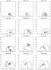Fig. 1 Time evolution of the largest avalanche event #1628 in the 2-D cellular automaton simulation with grid size N = 642. The 12 panels show snapshots at particular burst times from t = 26 to t = 690 when the energy dissipation rate peaked. Active nodes where energy dissipation occurs at time t are visualized with black and grey points, depending on the energy dissipation level. The starting point of the avalanche occurred at pixel (x,y) = (41,4), which is marked with a cross. The time-integrated envelop of the avalanche is indicated with a solid contour, and the diffusive avalanche radius r(t) = t1/2 is indicated with a dashed circle. The temporal evolution is shown in a movie available in the on-line version.

2.2. The fractal geometry of instantaneous energy dissipation

While we established the space-filling nature of the time-integrated avalanche area with a (non-fractal) Euclidean dimension in the foregoing section, we will now, in contrast, derive the theorem that the instantaneous area of energy dissipation in avalanches is fractal. It is actually a key concept of SOC systems that the spatial structure of avalanches is fractal. Bak & Chen (1989) express this most succintly in their abstract: “Fractals in nature originate from self-organized critical dynamical processes”.

As it can be seen from the snapshots of an evolving avalanche shown in Fig. 1, the instantaneous areas of energy dissipation cover a fraction of the solid area a(t) that is encompassed by the diffusive boundary. A detailed inspection of the shapshots shown in Fig. 1 even reveals a checkerboard pattern of instantaneous avalanche maps that emphasizes the fractal topology of cellular automaton avalanches. We make now the second major assumption that the area A(t) of instantaneous energy dissipation de(t)/dt is fractal, or that the volume V(t) for 3-D avalanches is fractal, respectively. To simplify the nomenclature, we will generally refer to the fractal volume V_S in S-dimensional Euclidean space, which corresponds to V₃ = V for fractal volumes in 3-D space, to V₂ = A for fractal areas in 2-D space, and V₁ = X for fractal lengths in 1-D space. (Note that we use uppercase symbols V,A,X for fractal parameters, while we use lowercase symbols v,a,x for non-fractal Euclidean parameters.) A fractal volume V_S can be defined by the Hausdorff dimension D_S in S-dimensional Euclidean space, 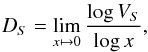${\mathit{D}}_{\mathit{S}}\mathrm{=}\underset{\mathit{x}\mathrm{}\mathrm{\to }\mathrm{0}}{\lim }\frac{\log {\mathit{V}}_{\mathit{S}}}{\log \mathit{x}}\mathit{,}$(5)where V_S is the fractal volume with Euclidean scale x, or by the scaling law, ${\mathit{V}}_{\mathit{S}}\mathrm{\propto }{\mathit{x}}^{{\mathit{D}}_{\mathit{S}}}\mathit{.}$(6)In Fig. 2 we demonstrate the fractal nature of the 12 instantaneous avalanche snapshots shown in Fig. 1. We rebin the avalanche area into macropixels with sizes of Δx_i = 2ⁱ,i = 0,...,3 (or x = 1,2,4,8), measure the number of macropixels A_i that cover the instantaneous avalanche area, use the diffusive scaling x(t) ∝ t^1/2 (Eq. (1)) for the rebinned length units x_i = x(t)/Δx_i, and determine the Hausdorff dimemsion D₂ from the linear regression fit log (A_i) = D₂log (x_i). We find that that the 4 datapoints for each of the 12 cases exhibit a linear relationship, which proves the fractality of the avalanche areas. The average fractal dimension of the 12 timesteps shown in Figs. 1 and 2 is D₂ = 1.43 ± 0.17.

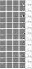Fig. 2 Determination of the fractal dimension D2 = log Ai/log xi for the instantaneous avalanche sizes of the 12 time steps of the avalanche event shown in Fig. 1. Each row is a different time step and each column represents a different binning of macropixels (Δxi = 1,2,4,8). The fractal dimension is determined by a linear regression fit shown on the right-hand side. The mean fractal dimension of the 12 avalanche snapshots is D2 = 1.43 ± 0.17.

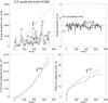Fig. 3 Time evolution of the largest avalanche event #1628 in the 2-D cellular automaton simulation with grid size N = 642. The time profiles include the instantaneous energy dissipation rate f(t) = de/dt (top left), the time-integrated total energy e(t) (bottom left), the instantaneous fractal dimension D2(t) (top right), and the radius of the avalanche area r(t) (bottom right). The observed time profiles from the simulations are outlined in solid linestyle and the theoretically predicted average evolution in dashed linestyle. The statistically predicted values of the instantaneous energy dissipation rate f(t) ∝ t3/4 (dotted curve) and peak energy dissipation rate p(t) ∝ t1 (dashed curve) after a time interval t are also shown (top left panel). The 12 time labels from 26 to 690 (top left frame) correspond to the snapshot times shown in Fig. 1.

We measure now the fractal dimension D₂ of the instantaneous energy dissipation volume in the 2-D avalanche for all 700 time steps of its duration, shown for 12 time instants in Fig. 1. The unstable nodes (signifying instantaneous energy dissipation) are counted in each time step, which yield a number for the fractal volume or area A(t) = V₂(t), while the size x of the encompassing box is determined from the area of the time-integrated avalanche, i.e., $\mathit{x}\mathrm{\left(}\mathit{t}\mathrm{\right)}\mathrm{=}\sqrt{\mathit{a}\mathrm{\left(}\mathit{t}\mathrm{\right)}}$, which yields the time evolution of the fractal dimension D₂(t) = log  [V₂(t)] /log  [x(t)]  (Eq. (5)) as a function of time, shown in the top right panel in Fig. 3. The fractal dimension D₂(t) fluctuates around a constant mean value of D₂ = 1.45 ± 0.13, which is close to the arithmetic mean of the minimum dimension D_2,min ≈ 1 and maximum Euclidean limit D_2,max = 2, i.e.  ⟨ D₂ ⟩  ≈ (D_2,min + D_2,max)/2 = 3/2. This corroborates our second major assumption that the instantaneous volume of energy dissipation is fractal, and that the fractal dimension can be approximated by a mean (time-independent and size-independent) constant during the evolution of avalanches, in the statistical average.

If we moreover define a mean energy dissipation rate quantum  ⟨ ΔE ⟩  per unstable node, which is indeed almost a constant for a cellular automaton model near the critical state, we expect a scaling of the instantaneous dissipation rate (or flux) f(t) that is proportional to the instantaneous dissipation volume V_S (with Eq. (6)), 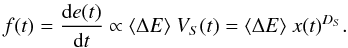$\mathit{f}\mathrm{\left(}\mathit{t}\mathrm{\right)}\mathrm{=}\frac{\mathrm{d}\mathit{e}\mathrm{\left(}\mathit{t}\mathrm{\right)}}{\mathrm{d}\mathit{t}}\mathrm{\propto }\mathrm{⟨}\mathrm{\Delta }\mathit{E}\mathrm{⟩}{\mathit{V}}_{\mathit{S}}\mathrm{\left(}\mathit{t}\mathrm{\right)}\mathrm{=}\mathrm{⟨}\mathrm{\Delta }\mathit{E}\mathrm{⟩}\mathit{x}\mathrm{(}\mathit{t}{\mathrm{)}}^{{\mathit{D}}_{\mathit{S}}}\mathit{.}$(7)Combining this with the diffusive expansion of the boundary x(t) ∝ t^1/2 (Eq. (1)), we can then predict the average time evolution of the energy dissipation rate f(t) = de(t)/dt, $\mathit{f}\mathrm{\left(}\mathit{t}\mathrm{\right)}\mathrm{=}\frac{\mathrm{d}\mathit{e}\mathrm{\left(}\mathit{t}\mathrm{\right)}}{\mathrm{d}\mathit{t}}\mathrm{\propto }\mathrm{⟨}\mathrm{\Delta }\mathit{E}\mathrm{⟩}{\mathit{t}}^{\mathrm{(}{\mathit{D}}_{\mathit{S}}\mathit{/}\mathrm{2}\mathrm{)}}\mathit{.}$(8)Integrating Eq. (8) in time, we obtain the time evolution of the total dissipated energy, e(t), $\mathit{e}\mathrm{\left(}\mathit{t}\mathrm{\right)}\mathrm{=}{\mathrm{\int }}_{\mathrm{0}}^{\mathit{t}}\frac{\mathrm{d}\mathit{e}\mathrm{\left(}\mathit{\tau }\mathrm{\right)}}{\mathrm{d}\mathit{\tau }}\mathrm{d}\mathit{\tau }\mathrm{\propto }{\mathrm{\int }}_{\mathrm{0}}^{\mathit{t}}{\mathit{\tau }}^{{\mathit{D}}_{\mathit{S}}\mathit{/}\mathrm{2}}\mathrm{d}\mathit{\tau }\mathrm{=}{\mathit{t}}^{\mathrm{(}\mathrm{1}\mathrm{+}{\mathit{D}}_{\mathit{S}}\mathit{/}\mathrm{2}\mathrm{)}}\mathit{.}$(9)Hence, for our 2-D avalanche (with D₂ = 3/2) we expect an evolution of e(t) ∝ t^(7/4), which indeed closely matches the actually simulated cellular automaton case, as we see in Fig. 3 (bottom left panel). The time evolution of the energy dissipation rate is shown in Fig. 3 (top left panel), which fluctuates strongly during the entire avalanche, but follows in the statistical average the predicted evolution de(t)/dt ∝ t^D₂/2 = t^(3/4) for D₂ ≈ 3/2. Note that our analytical expressions of the time evolution of avalanches, such as the linear size x(t) (Eq. (1)), the instantaneous energy dissipation rate f(t) (Eqs. (7), (8)), or the total dissipated energy e(t) (Eq. (9)), do not predict the specific evolution of a single avalanche event, but rather the statistical expectation value of a large ensemble of avalanches, similar to the statistical nature of the diffusive random walk model (Eq. (1)).

The time evolution of the instantaneous energy dissipation rate f(t) fluctuates strongly, as it can be seen in for the largest avalanche simulated in a cellular automaton model (Fig. 3, top left panel). We might estimate the peak values that can be obtained statistically (after a time duration t) from the optimum conditions when the fractal filling factor of the avalanche reaches a near-Euclidean filling, i.e., in the limit of D_S → S. Replacing the fractal dimension D_S by the Euclidean limit S in Eqs. (7) and (8) yields then (as an upper limit) an expectation value for the peak p(t), $\mathit{p}\mathrm{\left(}\mathit{t}\mathrm{\right)}\mathrm{\propto }\mathrm{⟨}\mathrm{\Delta }\mathit{E}\mathrm{⟩}{\mathit{V}}_{\mathit{S}}^{\max }\mathrm{\left(}\mathit{t}\mathrm{\right)}\mathrm{\propto }\mathrm{⟨}\mathrm{\Delta }\mathit{E}\mathrm{⟩}\mathit{x}\mathrm{(}\mathit{t}{\mathrm{)}}^{\mathit{S}}\mathrm{\propto }\mathrm{⟨}\mathrm{\Delta }\mathit{E}\mathrm{⟩}{\mathit{t}}^{\mathrm{(}\mathit{S}\mathit{/}\mathrm{2}\mathrm{)}}\mathit{.}$(10)Denoting the energy dissipation rate in the statistical average after time t = T with with F = f(t = T), the peak energy dissipation rate with P = p(t = T), and the total energy of the avalanche with E = e(t = T), it follows from Eqs. (8)–(10) that E ∝ FT = P^D_S/ST, and we expect then the following correlations between the three parameters E, F, P and T for an ensemble of avalanches, $\begin{array}{c}\\ \mathit{E}\mathrm{\propto }{\mathit{T}}^{\mathrm{1}\mathrm{+}{\mathit{D}}_{\mathit{S}}\mathit{/}\mathrm{2}}\\ \mathit{F}\mathrm{\propto }{\mathit{T}}^{{\mathit{D}}_{\mathit{S}}\mathit{/}\mathrm{2}}\\ \mathit{P}\mathrm{\propto }{\mathit{T}}^{\mathit{S}\mathit{/}\mathrm{2}}\mathit{.}\end{array}$(11)For instance, for a 2-D avalanche with an average fractal dimension of D₂ = 3/2 we expect the following two correlations, E ∝ T^7/4, F ∝ T^3/4, and P ∝ T¹ (see Fig. 3). The powerlaw indices for the correlated parameters are listed for the three Euclidean dimensions S = 1,2,3 separately in Table 1.

2.3. Occurrence frequency distributions

Considering the probability of an avalanche with volume V, the statistical likelihood simply scales reciprocally to the volume size V, if avalanches are equally likely in every space location of a uniform volume V₀ of a system in a (self-organized) critical state. This is illustrated in Fig. 4. For the 1-D Euclidean space, n = 1 avalanche can happen with the maximum size L = L₀ of the system (top left), n = 2 avalanches with the half size L = L₀/2, or n = 4 avalanches for a quarter size L = L₀/4. For the 2-D Euclidean space, the number of possible avalanches that can be fit into the total area A₀ of the system is n = 1 for A = A₀, n = 2² = 4 for A = A₀/2, or n = 2⁴ = 16 for A = A₀/4 (second row). For the 3-D Euclidean space we have, correspondingly, n = 1 for V = V₀, n = 2³ = 8 for cubes of half size L = L₀/2, and n = 4³ = 64 for quarter-size cubes with L = L₀/4 (bottom row). So, generalizing to S = 1,2,3 dimensions, we can express the probability for an avalanche of size L and volume V_S = L^S as, $\mathit{N}\mathrm{\left(}\mathit{L}\mathrm{\right)}\mathrm{\propto }{\mathit{V}}_{\mathit{S}}^{-1}\mathrm{\propto }{\mathit{L}}^{\mathrm{-}\mathit{S}}\mathit{.}$(12)This simple probability argument is based on the assumption that the number or occurrence frequency of avalanches is equally likely throughout the system, so it assumes a homogeneous distribution of critical states across the entire system.

The occurrence frequency distribution of length scales, N(L) ∝ L ^− S (Eq. (12)), serves as a primary distribution function from which all other occurrence frequency distribution functions N(x) can the derived that have a functional relationship to the primary parameter L. First we can calculate the occurrence frequency distribution of avalanche time scales, by using the diffusive boundary propagation relationship L(T) ∝ T^1/2 (Eq. (4)), by substituting the variable T for L in the distribution N(L) (Eq. (12)), $\mathit{N}\mathrm{\left(}\mathit{T}\mathrm{\right)}\mathrm{d}\mathit{T}\mathrm{=}\mathit{N}\mathrm{\left(}\mathit{L}\mathrm{\right[}\mathit{T}\mathrm{\left]}\mathrm{\right)}\left|\frac{\mathrm{d}\mathit{L}}{\mathrm{d}\mathit{T}}\right|\mathrm{d}\mathit{T}\mathrm{\propto }{\mathit{T}}^{\mathrm{-}\mathrm{\left[}\mathrm{\right(}\mathrm{1}\mathrm{+}\mathit{S}\mathrm{)}\mathit{/}\mathrm{2}\mathrm{]}}\mathrm{d}\mathit{T}\mathit{.}$(13)Subsequently we can derive the occurrence frequency distribution function N(F) for the statistically average energy dissipation rate F = f(t = T) using the relationship F(T) ∝ T^D_S/2 (Eq. (11)), $\mathit{N}\mathrm{\left(}\mathit{F}\mathrm{\right)}\mathrm{d}\mathit{F}\mathrm{=}\mathit{N}\mathrm{\left(}\mathit{T}\mathrm{\right[}\mathit{F}\mathrm{\left]}\mathrm{\right)}\left|\frac{\mathrm{d}\mathit{T}}{\mathrm{d}\mathit{F}}\right|\mathrm{d}\mathit{F}\mathrm{\propto }{\mathit{F}}^{\mathrm{-}\mathrm{[}\mathrm{1}\mathrm{+}\mathrm{(}\mathit{S}\mathrm{-}\mathrm{1}\mathrm{)}\mathit{/}{\mathit{D}}_{\mathit{S}}\mathrm{]}}\mathrm{d}\mathit{F,}$(14)the occurrence frequency distribution function of the peak energy dissipation rate P using the relationship relationship P(T) ∝ T^S/2 (Eq. (11)), $\mathit{N}\mathrm{\left(}\mathit{P}\mathrm{\right)}\mathrm{d}\mathit{P}\mathrm{=}\mathit{N}\mathrm{\left(}\mathit{T}\mathrm{\right[}\mathit{P}\mathrm{\left]}\mathrm{\right)}\left|\frac{\mathrm{d}\mathit{T}}{\mathrm{d}\mathit{P}}\right|\mathrm{d}\mathit{P}\mathrm{\propto }{\mathit{P}}^{\mathrm{-}\mathrm{[}\mathrm{2}\mathrm{-}\mathrm{1}\mathit{/}\mathit{S}\mathrm{]}}\mathrm{d}\mathit{P,}$(15)and the occurrence frequency distribution function N(E) for the total energy E using the relationship E(T) ∝ T^1 + D_S/2 (Eq. (11)), $\mathit{N}\mathrm{\left(}\mathit{E}\mathrm{\right)}\mathrm{d}\mathit{E}\mathrm{=}\mathit{N}\mathrm{\left(}\mathit{T}\mathrm{\right[}\mathit{E}\mathrm{\left]}\mathrm{\right)}\left|\frac{\mathrm{d}\mathit{T}}{\mathrm{d}\mathit{E}}\right|\mathrm{d}\mathit{E}\mathrm{\propto }{\mathit{E}}^{\mathrm{-}\mathrm{[}\mathrm{1}\mathrm{+}\mathrm{(}\mathit{S}\mathrm{-}\mathrm{1}\mathrm{)}\mathit{/}\mathrm{(}{\mathit{D}}_{\mathit{S}}\mathrm{+}\mathrm{2}\mathrm{\left)}\mathrm{\right]}}\mathrm{d}\mathit{E}\mathit{.}$(16)Interestingly, this derivation yields naturally powerlaw functions for all parameters L, T, F, P, and E, which are the hallmarks of SOC systems. In summary, if we denote the occurrence frequency distributions N(x) of a parameter x with a powerlaw distribution with power index α_x, $\mathit{N}\mathrm{\left(}\mathit{x}\mathrm{\right)}\mathrm{d}\mathit{x}\mathrm{\propto }{\mathit{x}}^{\mathrm{-}{\mathit{\alpha }}_{\mathit{x}}}\mathrm{d}\mathit{x,}$(17)we have the following powerlaw coefficients α_x for the parameters x = T,F,P, and E, 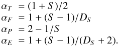$\begin{array}{c}\\ {\mathit{\alpha }}_{\mathit{T}}& \mathrm{=}\mathrm{(}\mathrm{1}\mathrm{+}\mathit{S}\mathrm{)}\mathit{/}\mathrm{2}\\ {\mathit{\alpha }}_{\mathit{F}}& \mathrm{=}\mathrm{1}\mathrm{+}\mathrm{(}\mathit{S}\mathrm{-}\mathrm{1}\mathrm{)}\mathit{/}{\mathit{D}}_{\mathit{S}}\\ {\mathit{\alpha }}_{\mathit{P}}& \mathrm{=}\mathrm{2}\mathrm{-}\mathrm{1}\mathit{/}\mathit{S}\\ {\mathit{\alpha }}_{\mathit{E}}& \mathrm{=}\mathrm{1}\mathrm{+}\mathrm{(}\mathit{S}\mathrm{-}\mathrm{1}\mathrm{)}\mathit{/}\mathrm{(}{\mathit{D}}_{\mathit{S}}\mathrm{+}\mathrm{2}\mathrm{)}\mathit{.}\end{array}$(18)For instance, for our 2-D cellular automaton model with S = 2 and D_S = 3/2 we predict powerlaw slopes of α_T = 3/2 = 1.5, α_F = 5/3 ≈ 1.67, α_P = 3/2 = 1.5, and α_E = 9/7 ≈ 1.28. The powerlaw coefficients α_x are summarized in Table 1 separately for each Euclidean dimension S = 1,2,3.

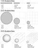Fig. 4 Schematic diagram of the Euclidean volume scaling of the diffusive avalanche boundaries, visualized as circles or spheres in the three Euclidean space dimensions S = 1,2,3. The Euclidean length scale x of subcubes decreases by a factor 2 in each step (xi = 2 − i,i = 0,1,2), while the number of subcubes increases by ni = (2i)S, defining a probability of $\mathit{N}\mathrm{\left(}{\mathit{x}}_{\mathit{i}}\mathrm{\right)}\mathrm{\propto }{\mathit{x}}_{\mathit{i}}^{\mathrm{-}\mathit{S}}$ for each avalanche size with size xi.

2.4. Estimating the fractal dimension of cellular automatons

The dynamics of SOC systems is often simulated on computers with cellular automaton codes, which have a S-dimensional lattice of nodes, where a discretized mathematical redistribution rule is applied once a local instability threshold is surpassed (e.g., Bak et al. 1987; Lu & Hamilton 1991; Charbonneau et al. 2001). Avalanches in such cellular automaton models propagate via nearest-neighbor interactions, which includes (2S + 1) nodes in a S-dimensional lattice grid: one element is the unstable node, and there are 2S next neighbors. For instance, a 1-dimensional grid in Euclidian space with dimension S = 1 has (2S + 1) = 3 nodes involved in a single nearest-neighbor relaxation step, a 2-dimensional grid (S = 2) has (2S + 1) = 5 nodes, and a 3-dimensional grid (S = 3) has (2S + 1) = 7 nodes (Fig. 5).

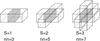Fig. 5 The fractal geometry of next-neighbor interactions are shown for a cellular automaton lattice model for Euclidian dimensions S = 1 (left), S = 2 (middle), and S = 3 (right). The unstable node is shaded with grey, and the next neighbor nodes in white. The total number nn of nodes involved in a local redistribution rule scales as nn = 2S + 1 with the Euclidean dimension S.

How can we estimate the fractal dimension for avalanches in such a lattice-based cellular automaton model? The minimum fractal dimension of a growing 3-D avalanche corresponds to a 1-D linear structure, D_3,min = 1, because avalanches evolve by iterative propagation from one node to the next-neighbor node, so a contiguous linear path from one node to the next neighbor is about the sparsest spatial structure that still enables avalanche growth in a SOC model. If the linear avalanche path would be discontinuous (D_S < 1), the avalanche is likely to die out due to a lack of unstable next neighbors, so D_S,min ≈ 1 represents practically a lower cutoff, which does not exclude occasional values of D_S < 1 (fractal dust). At the other extreme, when all nodes are close to the instability threshold, an avalanche can affect all next neighbors and grow as a nearly space-filling structure with a maximum fractal dimension of D_S,max = S that equals the Euclidean space dimension S. The mean average fractal dimension  ⟨ D_S ⟩  can then be estimated from the geometric mean of the minimum V_S,min and maximum fractal volume V_S,max, which is equivalent to the arithmetic mean of the minimum D_S,min and maximum fractal dimension D_S,max (Eq. (5)), 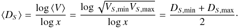$\mathrm{⟨}{\mathit{D}}_{\mathit{S}}\mathrm{⟩}\mathrm{=}\frac{\log \mathrm{⟨}\mathit{V}\mathrm{⟩}}{\log \mathit{x}}\mathrm{=}\frac{\log \sqrt{{\mathit{V}}_{\mathit{S,}\min }{\mathit{V}}_{\mathit{S,}\max }}}{\log \mathit{x}}\mathrm{=}\frac{{\mathit{D}}_{\mathit{S,}\min }\mathrm{+}{\mathit{D}}_{\mathit{S,}\max }}{\mathrm{2}}\mathrm{·}$(19)From this we predict the following mean fractal dimensions  ⟨ D_S ⟩  in different Euclidean spaces with dimensions S = 1,2,3, $\begin{array}{c}\\ \mathrm{⟨}{\mathit{D}}_{\mathrm{1}}\mathrm{⟩}\mathrm{=}\mathrm{(}\mathrm{1}\mathrm{+}\mathrm{1}\mathrm{)}\mathit{/}\mathrm{2}\mathrm{=}\mathrm{1}\\ \mathrm{⟨}{\mathit{D}}_{\mathrm{2}}\mathrm{⟩}\mathrm{=}\mathrm{(}\mathrm{1}\mathrm{+}\mathrm{2}\mathrm{)}\mathit{/}\mathrm{2}\mathrm{=}\mathrm{3}\mathit{/}\mathrm{2}\\ \mathrm{⟨}{\mathit{D}}_{\mathrm{3}}\mathrm{⟩}\mathrm{=}\mathrm{(}\mathrm{1}\mathrm{+}\mathrm{3}\mathrm{)}\mathit{/}\mathrm{2}\mathrm{=}\mathrm{2.}\end{array}$(20)or more generally as a function of the Euclidean space dimension S, $\mathrm{⟨}{\mathit{D}}_{\mathit{S}}\mathrm{⟩}\mathrm{\approx }\frac{\mathrm{(}\mathrm{1}\mathrm{+}\mathit{S}\mathrm{)}}{\mathrm{2}} \mathrm{for}\mathit{S}\mathrm{=}\mathrm{1}\mathit{,}\mathrm{2}\mathit{,}\mathrm{3.}$(21)Using these estimates of the mean fractal dimension  ⟨ D_S ⟩  into Eq. (18) we obtain the numerical values given in Table 1. Note, that this estimate of the mean fractal dimension is only an approximation, because the lower limit D_S,min ≈ 1 is not rigorously derived from probability theory. However, as the example in Fig. 3 shows, the estimated fractal dimension of D₂ = 1.5 comes close to the observed mean value of  ⟨ D₂ ⟩  = 1.45 ± 0.13 in this avalanche.

SOC systems that are different from the isotropic cellular automaton model we are using here may have different fractal dimensions. Thus our theoretical prediction of the mean fractal dimension applies only to SOC systems with similar isotropic next-neighbor redistribution rules. For any observed SOC system, the fractal dimension D_S can be empirically determined by measuring the powerlaw slopes α_F or α_E, which are a function of the fractal dimension D_S (Eq. (18)).

3. Cellular automaton simulations

3.1. Numerical cellular automaton code

An isotropic cellular automaton model that mimics a SOC system was originally conceived by Bak et al. (1987, 1988) and first applied to solar flares by Lu & Hamilton (1991). A version generalized to S = 1,2,3 dimensions is given in Charbonneau et al. (2001) and is also summarized in Aschwanden (2011).

The numerical simulations of cellular automaton models take place in a S-dimensional cartesian grid, where nodes are localized by discretized coordinates, say with x_ijk in S = 3, and a physical scalar quantity B_ijk = B(x = x_ijk) is assigned to each node. The dynamics of the system is initiated by quantized energy inputs δB(t) at random locations x_ijk with a constant rate as a function of time. At each time step t and spatial node x_ijk, the local stability is checked by measuring the local S-dimensional “curvature” (Charbonneau et al. 2001) with respect to the next neighbor cells (nodes) x_nn = x_{i ± 1,j ± 1,k ± 1}, $\mathrm{\Delta }{\mathit{B}}_{\mathit{ijk}}\mathrm{=}{\mathit{B}}_{\mathit{ijk}}\mathrm{-}\frac{\mathrm{1}}{\mathrm{2}\mathit{S}}\begin{array}{}\sum \end{array}{\mathit{B}}_{\mathit{nn}}\mathit{.}$(22)Most nodes are stable at a particular time if the system is driven slowly, say with an input rate δB/ ⟨ B_ijk ⟩  ≪ 1 (Charbonneau et al. 2001). The system is defined to be stable, as long as the local gradients are smaller than some critical threshold value B_c. However, once a local gradient exceeds the critical value, i.e., ΔB_ijk ≥ B_c, a mathematical redistribution rule is applied that smoothes out the local gradient and makes it stable again. The redistribution rule simply spreads the difference ΔB_ijk (or the threshold B_c) equally to the next neighbors (in an isotropic cellular automaton model), ${{B}}_{\mathit{ijk}}\mathrm{}\mathrm{\to }{{B}}_{\mathit{ijk}}\mathrm{-}\frac{\mathrm{2}\mathit{S}}{\mathrm{2}\mathit{S}\mathrm{+}\mathrm{1}}{B}\mathrm{c}\mathit{,} {{B}}_{\mathit{nn}}\mathrm{}\mathrm{\to }{{B}}_{\mathit{nn}}\mathrm{+}\frac{\mathrm{1}}{\mathrm{2}\mathit{S}\mathrm{+}\mathrm{1}}{B}\mathrm{c}\mathit{.}$(23)Note that the amount of the redistributed quantity is the threshold energy B_c in the models of Lu et al. (1993) and Charbonneau et al. (2001), while it is the (larger) amount of the actual gradient ΔB_ijk in the original model of Lu & Hamilton (1991). If the node is unstable, then the actual gradient is larger than the critical gradient, rather than smaller. This was modified in a later paper (Lu et al. 1993) by redistributing the threshold gradient rather than the full gradient, presumably due to numerical instabilities (Liu et al. 2002). This redistribution rule is conservative, in the sense that the quantity B is conserved after every redistribution step, because the same amount is transferred to the next neighbors that is taken away from the central cell. However, although the scalar field quantity B is conserved, the energy B² is not conserved after a redistribution step, because of the nonlinear (quadratic) dependence assumed, which was introduced in analogy to the magnetic field energy density E_mag = B²/8π. In fact, every redistribution of |ΔB| > B_c dissipates energy from the system, by an amount of (Charbonneau et al. 2001), $\mathit{E}\mathrm{=}\frac{\mathrm{2}\mathit{S}}{\mathrm{2}\mathit{S}\mathrm{+}\mathrm{1}}\left(\frac{\mathrm{2}\mathrm{\left|}\mathrm{\Delta }\mathit{B}\mathrm{\right|}}{{\mathit{B}}_{\mathrm{c}}}\mathrm{-}\mathrm{1}\right){\mathit{B}}_{\mathrm{c}}^{\mathrm{2}}\mathit{.}$(24)Thus, the minimum amount of dissipated energy is for |ΔB| ≳ B_c, when the threshold B_c is infinitesimally exceeded by |ΔB|, ${\mathit{E}}_{\min }\mathrm{=}\frac{\mathrm{2}\mathit{S}}{\mathrm{2}\mathit{S}\mathrm{+}\mathrm{1}}{\mathit{B}}_{\mathrm{c}}^{\mathrm{2}}\mathit{.}$(25)Once a node x_ijk is found to be unstable, the check of unstable cells propagates to the next neighbors x_nn = x_{i ± 1,j ± 1,k ± 1} in the next time step and all unstable neighbor cells are subject to the redistribution rule, and progressively continues to the next neighbors each time step until all cells are stable again. Such a chain reaction of next-neighbor redistributions is called an avalanche event (see examples in Fig. 4). Note that a minimum avalanche has to include at least one redistribution step.

In this study the author coded independently such a cellular automaton algorithm according to the specifications given in Sect. 2.5 of Charbonneau et al. (2001) and it was run with exactly the same system parameters, such as the input quantity σ₁ ≤ δB ≤ σ₂ homogeneously distributed in the range of σ₁ =  −0.2 to σ₂ = 0.8, the threshold quantity B_c = 5, with grid sizes of N = 128 and 256 in one dimension (S = 1), N = 32 and 64 in two dimensions (S = 2), and N = 16 and 24 in three dimensions (S = 3). We sampled the total volumes V, energies E, peak energy dissipation rate P, and durations T of avalanches and were able to reproduce the results given in Charbonneau et al. (2001) consistently, although we used different random generators for the input, different time intervals for the initiation phase and onset of SOC (t_SOC = 3 × 10⁶ for N = 128 and S = 1; t_SOC = 15 × 10⁶ for N = 256 and S = 1; t_SOC = 5 × 10⁶ for N = 32 and S = 2; t_SOC = 41 × 10⁶ for N = 64 and S = 2; t_SOC = 4 × 10⁶ for N = 16 and S = 3; t_SOC = 15 × 10⁶ for N = 24 and S = 3), and slightly different powerlaw fitting procedures. In addition, we calculated also the fractal dimensions of the SOC avalanches from the avalanche volumes V and the size x of the enveloping Euclidean cube x^S, ${\mathit{D}}_{\mathit{S}}\mathrm{=}\frac{\log \mathrm{\left(}\mathit{V}\mathrm{\right)}}{\log \mathrm{\left(}\mathit{x}\mathrm{\right)}}\mathit{,}$(26)where x is the largest spatial scale that brackets the fractal avalanche volume in each spatial direction (x,y,z) of the S-dimensional Euclidean space. This definition is slightly different from the “radius of gyration” method employed in Charbonneau et al. (2001), but follows more the standard convention of fractal dimensions measured with box-counting methods. In the following we show the results from two runs in each dimension S = 1,2,3 and compare them with the theoretical predictions made in Sect. 2.

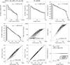Fig. 6 Cellular automaton simulations with a N = 256 1-D lattice produced by a numerical code according to Charbonneau et al. (2001). The frequency distributions of peak energy dissipation rate P, total energies E, time durations T, and fractal avalanche volumes V are shown along with the fitted powerlaw slopes. Correlations between the fractal dimension D1 and parameters E, P, and T are also shown, fitted in the ranges of P ≥ 50, E ≥ 50, T ≥ 5, and V ≥ 2. Only a representative subset of 2000 events are plotted in the scatterplots.

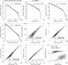Fig. 7 Cellular automaton simulations with a N = 642 2-D lattice produced by a numerical code according to Charbonneau et al. (2001). Representation otherwise similar to Fig. 6.

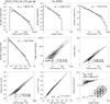Fig. 8 Cellular automaton simulations with a N = 242 3-D lattice produced by a numerical code according to Charbonneau et al. (2001). Representation otherwise similar to Figs. 6 and 7.

3.2. Occurrence frequency distributions

The results of occurrence frequency distributions and correlations are shown for a 1-D (Fig. 6), a 2-D (Fig. 7), and a 3-D cellular automaton code (Fig. 8), and listed in Table 2. We evaluated the powerlaw slopes by a weighted linear regression fit (weighted by the number of avalanche events per bin) by excluding undersampled bins (less than 20 events). Since the exact values depend sometimes on the fitted range, we vary the range of linear regression fits from the full range of the powerlaw part (indicated with black line in Figs. 6–8) to the upper half (indicated with grey line in Figs. 6–8) and calculate the average and standard deviations of the powerlaw slope values.

The values of the predicted and simulated powerlaw slopes are compiled in Table 2. First of all we notice an extremely good agreement (within a few percents) of the powerlaw slopes α_E, α_P, and α_T between our simulations and those of Charbonneau et al. (2001) and McIntosh et al. (2002), although we used different codes, initiation times t_SOC, and powerlaw fitting procedures. We performed the 1-D to 3-D runs with small cubes (N = 128,32,16) as well as with larger cubes (N = 256,64,24), which both give very consistent values (Table 2). In the following we quote only the values for the larger cubes, which are also shown in Figs. 6–8.

Considering the agreement between theory and simulations, there is a reasonable agreement for all three space dimensions S = 1,2,3. For the fractal dimension of avalanches we find D₂ = 1.60 ± 0.17 (predicted D₂ = 1.5) and D₃ = 1.94 ± 0.27 (predicted D₃ = 2.0), which are fully consistent with our theoretical estimate of D_S = (1 + S)/2 (Eq. (21)).

The relationship of the avalanche probability being reciprocal to the volume, N(L) ∝ L ^− S (Eq. (12)) is also approximately confirmed by the simulations, for which we find α_L = 0.88 ± 0.09 (predicted α_L = 1 for S = 1), α_L = 2.14 ± 0.18 (predicted α_L = 2 for S = 2), and α_L = 2.55 ± 0.10 (predicted α_L = 3 for S = 3), where the latter value has the largest error due to the smallest sizes of 3-D cubes with a dynamic range of only about 1 dex. Clearly this relationship agrees better for larger cubes (up to L = 256 in 1-D simulations). We have to add a caveat that finite-size effects are likely to restrict the size of avalanches at the system boundaries, especially for the 3D cellular automata runs which we run here with a size of 16³ and 24³ only. Also uncertainty estimates of the powerlaw slopes are less accurate for small dynamic ranges (i.e., small system size L here) and due to histogram binning. In the real world, however, finite-size effects may also cause modifications of powerlaw distributions, such as the maximum size of active regions or the vertical density scale height of coronal loops.

The total energy powerlaw slope α_E (Eq. (18)) fitted from the powerlaw distributions N(E) yields values of α_E = 1.06 ± 0.04 in 1-D (predicted α_E = 1.0), α_E = 1.48 ± 0.03 in 2-D (predicted α_E = 1.28), and α_E = 1.50 ± 0.06 in 3-D (predicted α_E = 1.5), which agree with the predictions within 6%, 16%, and 0%.

The peak energy dissipation rate powerlaw slope α_P (Eq. (18)) fitted from the powerlaw distributions N(P) yields values of α_P = 0.94 ± 0.18 in 1-D (predicted α_P = 1.0), α_P = 1.85 ± 0.06 in 2-D (predicted α_P = 1.5), and α_P = 1.96 ± 0.14 in 3-D (predicted α_P = 1.67), which agree with the predictions within 6%, 23%, and 17%.

The time duration powerlaw slope α_T (Eq. (18)) fitted from the powerlaw distributions N(T) yields values of α_T = 1.17 ± 0.02 in 1-D (predicted α_T = 1.0), α_T = 1.77 ± 0.18 in 2-D (predicted α_T = 1.5), and α_T = 1.76 ± 0.19 in 3-D (predicted α_T = 2.0), which agree with the predictions within 17%, 18%, and 12%.

Most occurrence frequency distributions are subject to a drop-off from an ideal powerlaw distribution due to finite-size effects. It is quite satisfactory that our simple first-order theory predicts most powerlaw slopes within an accuracy of order 10%. We have also to be aware that our first-order theory assumes that the fractal dimension of the energy release rate is a constant, while the simulated avalanches show a slight trend of increasing fractal dimensions D with size L, i.e., D₂ ≈ L^0.09 for S = 2, and D₃ ≈ L^0.19 for S = 3 (Figs. 7 and 8, bottom right). This slight trend of D_S(L) affects the powerlaw slopes α_P and α_E to be somewhat flatter for small avalanches than for larger ones, which represents a second-order effect and could be considered in a more refined theory.

3.3. SOC parameter correlations

An alternative method of testing our theory is (i) a determination of the power index β of correlated parameters x and y, i.e., y ∝ x^β, by linear regression fits log (y) ∝ log (y₀) + βlog (x); or (ii) by inferring them from the powerlaw slopes α_x and α_y of their occurrence frequency distributions, i.e., β = (α_x − 1)/(α_y − 1) (see derivation in Sect. 7.1.6 of Aschwanden 2011). The resulting values are listed for both methods in Table 3 (labeled with “Regression” and “Slopes”), for each 1-D, 2-D, and 3-D simulation run of our cellular automaton code. The linear regression fits are shown in the lower halves of Figs. 6–8. Note that truncations occurs for each parameter due to the effect of finite-size systems that have been used in the numerical simulations (L = 128 and 256 for 1-D; L = 32 and 64 for 2-D; and L = 16 and 24 for 3-D lattices). The minimum amount of dissipated energy for a threshold of B_c = 5 is E_min = 16.7 (for S = 1), E_min = 20 (for S = 2), and E_min = 21.4 (for S = 3), according to Eq. (25). Thus we perform the linear regression fits only in parameter ranges that are not too strongly affected by truncation effects, which is at durations T > 5, peak energy dissipation rate P > 50, and energies E > 50. To quantify an error of the linear regression fits, we perform fits of y(x), and with exchanged axes, x(y), and quote the mean and half difference for the two fits.

The correlation L ∝ T^1/2 (Eq. (4)) tests our assumption of a diffusive random walk for the propagating avalanche boundaries. For the theoretically expected value of the power index β_TL = 0.5 we find β_TL = 0.53−0.65 for 1-D avalanches, β_TL = 0.61−0.76 for 2-D avalanches, and β_TL = 0.48−0.53 for 3-D avalanches, which corroborates our assumption of a diffusive avalanche expansion.

For the correlation of the peak energy dissipation rate with the duration of an avalanche P ∝ T^β_TP we find β_TP = 0.67−0.73 for 1-D avalanches (predicted β_TP = 0.5), β_TP = 0.91−1.04 for 2-D avalanches (predicted β_TP = 1.0), and β_TP = 0.79−1.02 for 3-D avalanches (predicted β_TP = 1.5), which amounts to an agreement of  ≈ 30% for the 1-D case,  ≈ 3% for the 2-D case, and  ≈ 33% for the 3-D case. We suspect that a lot of avalanches are stopped at the boundary, which underestimates the peak energy dissipation rate and thus yields a systematically too high power index β_TP for the 3-D case.

For the correlation of the total energy with the duration of an avalanche E ∝ T^β_TE we find β_TE = 1.56−1.65 for 1-D avalanches (predicted β_TP = 1.5), β_TE = 1.61−1.82 for 2-D avalanches (predicted β_TP = 1.75), and β_TE = 1.51−1.75 for 3-D avalanches (predicted β_TP = 2.0), which amounts to an agreement of  ≈7% for the 1-D case,  ≈ 2% for the 2-D case, and  ≈18% for the 3-D case.

In summary, we find an overall agreement of order 10% between theory and numerical simulations for the power indexes of correlated parameters.

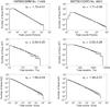Fig. 9 Occurrence frequency distributions of peak count rates P, durations T, and total counts E in solar flares observed with HXRBS/SMM during 1980–1989 (left panels) and with BATSE/CGRO during 1991–2000 (right panels) at energies  ≥ 25 keV (left).

4. Observations of solar flares

Let us turn now to some astrophysical observations to compare our theory and the results of cellular automaton simulations. Lu & Hamilton (1991) applied SOC theory and cellular automaton models for the first time to solar flares. They modeled the flare statistics from hard X-ray counts observed with the HXRBS detectors onboard SMM, which shows a powerlaw distribution extending over 4 orders of magnitude, with a powerlaw slope of α_P ≈ 1.8 for the peak count rate P (Dennis 1985). From their cellular automaton code they obtained powerlaw slopes of α_P ≈ 1.8 for the peak energy dissipation rate P, α_T ≈ 1.9 for the flare durations T, and α_E ≈ 1.4 for the total energies E. We re-analyzed the HXRBS/SMM dataset and obtain the values of α_P ≈ 1.73 ± 0.01 for the power P, α_T ≈ 2.29 ± 0.25 for the flare durations T, and α_E ≈ 1.56 ± 0.04 for the total energies E (Fig. 9, left). In addition we re-analyzed the BATSE/CGRO flare data set and obtained similar values of α_P ≈ 1.71 ± 0.06 for the peak energy dissipation rate P, α_T ≈ 2.02 ± 0.28 for the flare durations T, and α_E ≈ 1.49 ± 0.07 for the total energies E (Fig. 9, right).

Comparing the observed values with the theoretically predicted values of our 3-D fractal-diffusive SOC model (Sect. 2 and Table 1), we find the following ranges regarding the powerlaw slopes of the occurrence frequency distributions: flare durations α_T = 2.02 − 2.29 (predicted ${\mathit{\alpha }}_{\mathit{T}}^{\mathrm{theo}}\mathrm{=}\mathrm{2.00}$), peak energy dissipate rate α_P = 1.71 − 1.73 (predicted ${\mathit{\alpha }}_{\mathit{P}}^{\mathrm{theo}}\mathrm{=}\mathrm{1.67}$), and total energies α_E = 1.49 − 1.56 (predicted ${\mathit{\alpha }}_{\mathit{E}}^{\mathrm{theo}}\mathrm{=}\mathrm{1.50}$), Thus, theory and observations agree within a few percents, which is even better than the agreement of theory with the cellular automaton simulations in the 3D case (probably due to the limited grid size). The powerlaw index of the peak fluxes was found to vary with the solar cycle within a range of α_P ≈ 1.6 − 1.9 (Crosby et al. 1993; Biesecker 1994; Bai 1993; Aschwanden 2010a), which could indicate a variable degree of magnetic complexity that is manifested either in a time-dependent fractal dimension D_S, or threshold B_c of SOC events (Aschwanden 2010a,b).

Comparing the observed flux time profiles f(t) of the hard X-ray flux of large solar flares, they fluctuate erratically in a similar way as shown for the largest avalanche of cellular automaton simulations (Fig. 3, top left panel), as records with high time-resolution and high sensitivity show, e.g., observed with BATSE/CGRO (Aschwanden et al. 1998). The erratically fluctuating hard X-ray time profiles are generally interpreted in terms of the chromospheric energy dissipation rate of precipitating nonthermal electrons produced in magnetic reconnection processes, similar as we defined the instantaneous energy dissipation rate f(t) (Eq. (8)) in our cellular automaton model, while the associated soft X-ray time profile represents the thermal emission of the heated plasma, which is monotonically increasing during the impulsive flare phase because it represents the time integral of the heating rate according to the Neupert effect, similar as we defined the total dissipated energy e(t) (Eq. (9)) in our cellular automaton model. The positive index in the correlation of the peak energy dissipation rate P with the time duration T in our avalanche model, i.e., P ∝ T^S/2 (Eq. (10)), thus predicts that the hard X-ray peak flux is statistically the higher the longer a solar flare lasts (which is also known as “big-flare syndrome”).

A specific prediction is that in 3-D Euclidean space, regardless of the fractal dimension in the range of D₃ = 1,...,3, the distribution of flare energies is restricted to a relatively small range of ${\mathit{\alpha }}_{\mathit{E}}^{\mathrm{theo}}\mathrm{=}\mathrm{1.40}\mathrm{-}\mathrm{1.67}$, which is consistent with our observations of α_E = 1.49−1.56. The numerical value of the energy powerlaw slope of α_E ≈ 1.5 implies that the total energy of all flares is heavily weighted by the largest flares, while nanoflares contain only an insignificant amount of energy, unless the powerlaw slope is steeper than a critical value of α_E = 2 (Hudson 1991), which is an ongoing argument in the controversy of coronal heating by nanoflares. In order to make nanoflares dominant, a powerlaw slope of α_E > 2 is needed, which contradicts our model, since the maximum value cannot exceed α_E,max = 5/3 = 1.67, well below the critical limit of α_E = 2.

Interestingly, some cellular automaton simulations have been performed that actually produced significantly steeper powerlaw slopes, say in the order of α_E ≈ 3.0, which seems to contradict our conclusions. One simulation produced a broken powerlaw distribution with a slope of α_P = 3.5 for the smallest events, interpreted as nanoflare regime, while a flatter slope of α_P = 1.8 was found for the larger flares (Vlahos et al. 1995), a difference that is attributed to the anisotropic next-neighbor interactions applied therein. Another study simulated solar flare events as cascades of reconnecting magnetic loops, with the finding of a powerlaw slope of α_E = 3.0 for the released energies (Hughes et al. 2003). Interacting loops with a length scale L are bisected during a reconnection step into two shorter scales L/2, and the released energies are defined in terms of the length scale therein, i.e., E ∝ L, for which our model predicts indeed an occurrence frequency distribution of N(E) ∝ N(L) ∝ L ^− S ∝ L^-3 (Eq. (12)) for an Euclidean dimension S = 3, so it is fully consistent with our model if their energy definition is adopted. Discrepancies of powerlaw slopes among different studies can indeed often be explained in terms of inconsistent definitions of the energy quantity.

5. Conclusions

We developed an analytical theory for the statistical distributions and correlations of observable parameters of SOC events, which includes the avalanche length scale L, the time duration T, the peak P and energy dissipation rate F. The basic assumptions of our analytical model, which we call the fractal-diffusive SOC model, are the following:

• 1.

  Diffusive expansion of SOC avalanches: the radius r(t) or spatiallength scale L of an avalanche grows with time like the average of adiffusive random walk, which predicts a statistical correlation L ∝ T^1/2between the length scale L and time duration T of the avalanche.

• 2.

  Fractal energy dissipation rate: the complexity of random next-neighbor interactions in a critical SOC state can be characterized approximately with a fractal geometry. The volume (or area) of the instantaneous energy dissipation rate is assumed to have a fractal dimension D_S. The predicted statistical correlations are: F ∝ T^D_S/2, P ∝ T^S/2, and E ∝ T^1 + D_S/2.

• 3.

  Mean fractal dimension: the mean fractal dimension D_S for different Euclidean space dimensions S = 1,2,3 can be estimated from the arithmetic mean of the minimum dimension for a propagating avalanche, D_S,min ≈ 1, and the maximum (Euclidean) dimension D_S,max = S, which yields D_S ≈ (1 + S)/2.

• 4.

  Occurrence frequency distributions: equal probability of avalanches with size L at various spatial locations in a uniform, slowly-driven SOC system predicts a probability distribution of N(L) ∝ L ^− S. A direct consequence of this assumption, together with the other assumptions made above, yields a powerlaw function N(x) ∝ x ^− α_x for the occurrence frequency distributions of all parameters, which is the hallmark of a SOC system. The predicted powerlaw indices are: α_T = (1 + S)/2, α_F = 1 + (S − 1)/D_S, α_P = 2 − 1/S, and α_E = 1 + (S − 1)/(D_S + 2). Specifically, for applications to 3-D phenomena, absolute values are predicted for the powerlaw slopes α_L = 3, α_T = 2, and α_P = 1.67, while a range of α_E = 1.4,...,1.67 is expected for any fractal dimension in the range of 1 ≤ D₃ ≤ 3.

We have validated our theory by a detailed comparison with a set of SOC simulations using a specific form of a cellular automaton avalanche model (connectivity, stability threshold, redistribution rule, etc.), and found a good agreement between theory and numerical simulations, in the order of  ≈ 10% for the powerlaw slopes (α_L,α_T,α_E,α_P), the power indices of correlated parameters (β_TL,β_TP,β_TE), and the fractal dimensions D_S, for all three Euclidean space dimensions S = 1,2,3. Yet, at its most general level our theory is saying that the self-similarity of energy release statistics in such models is a direct reflection of the fractal nature of avalanches. The SOC flare model recently proposed by Morales & Charbonneau (2008, 2009) offers an interesting test of this conclusion. Their model, defined on a set of initially parallel magnetic flux strands, contained in a plane and subjected to random sideways deformation, with instability and readjustment occurring when the crossing angle of two flux strands exceeds some threshold angle. This model is thus strongly anisotropic, with pseudo-local stability and redistribution, in the sense that these operators now act on nearest-neighbors nodes located along each flux strand, rather than in the immediate spatial vicinity of the unstable sites. This is very different from the isotropic Lu et al. (1993)-type SOC model used here for validation. Yet, the results compiled in Table 2 of Morales & Charbonneau (2008) for their highest resolution simulations reveal that the theoretical occurrence frequency distributions obtained herein, do hold within the stated uncertainties on the power-law fits. Likewise, the power indices of the correlated parameters also agree with theory within the inferred uncertainties. This provides additional empirical support to our conjecture that the fractal-diffusive SOC model does represent a robust characterization of avalanche energy release in SOC systems in general. However, it should be remembered that the inferred scaling laws are only valid for a slowly-driven SOC system, while alternative SOC systems with time-variable drivers or non-stationary input rates exhibit modified occurrence frequency and waiting time distributions (Charbonneau et al. 2001; Norman et al. 2001), which was also found in solar observations extending over multiple solar cycles (Crosby et al. 1993; Biesecker 1994; Bai 1993; Aschwanden 2010a).

What other predictions can be made from our analytical model? For SOC processes in 3-D space, which is probably the most common application in the real world, the mean fractal dimension is predicted to be D₃ ≈ 2.0, which can be tested by measurements of fractal dimensions in observations. The 20 largest solar flares observed with TRACE have been analyzed in this respect and an area fractal dimension of D₂ = 1.89 ± 0.05 was found at the flare peaks, which translates into a value of D₃ = 2.10 ± 0.14 if we use an anisotropic flare arcade model (Aschwanden & Aschwanden 2008a). The distribution of flare energies is predicted to have a powerlaw slope of α_E = 1.50, which closely matches the observed statistics of solar flare hard X-ray emission (α_E ≈ 1.49 − 1.56). Since this value is undisputably below the critical limit α = 2 of the energy integral, the total released energy is contained in the largest flares and thus rules out any significant nanoflare heating of the solar corona. Another prediction, that we did not test here with solar flare data, is the diffusive flare size scaling. Straightforward tests could be carried out by gathering statistics of the flare size evolution during individual flares (which are predicted to scale as x(t) ∝ t^1/2), as well as from the statistics of a large sample of flares, which is predicted to show a correlation L ∝ T^1/2. The application of our fractal-diffusive SOC model to solar flares implies that the subsequent triggering of local magnetic reconnection events during a flare occurs as a diffusive random walk. A similar finding of diffusive random walk was also found in the turbulent flows of magnetic bright points in the lanes between photospheric granular convection cells (Lawrence et al. 2001). The spatio-temporal scaling of the diffusive random walk predicts also the size, duration, and energy of the largest flare, which is likely to be constrained by the size ${\mathit{L}}_{\mathrm{AR}}\mathrm{\propto }{\mathit{T}}_{\max }^{\mathrm{1}\mathit{/}\mathrm{2}}$ of the largest active region.

Online material

Movie of Fig. 1 Access here

Acknowledgments

The author thanks Paul Charbonneau for helpful discussions and contributions. This work is partially supported by NASA grant NAG5-13490 and NASA TRACE contract NAS5-38099. We acknowledge access to solar mission data and flare catalogs from the Solar Data Analysis Center (SDAC) at the NASA Goddard Space Flight Center (GSFC).

References

All Tables

All Figures

Fig. 1 Time evolution of the largest avalanche event #1628 in the 2-D cellular automaton simulation with grid size N = 642. The 12 panels show snapshots at particular burst times from t = 26 to t = 690 when the energy dissipation rate peaked. Active nodes where energy dissipation occurs at time t are visualized with black and grey points, depending on the energy dissipation level. The starting point of the avalanche occurred at pixel (x,y) = (41,4), which is marked with a cross. The time-integrated envelop of the avalanche is indicated with a solid contour, and the diffusive avalanche radius r(t) = t1/2 is indicated with a dashed circle. The temporal evolution is shown in a movie available in the on-line version.

In the text

Fig. 2 Determination of the fractal dimension D2 = log Ai/log xi for the instantaneous avalanche sizes of the 12 time steps of the avalanche event shown in Fig. 1. Each row is a different time step and each column represents a different binning of macropixels (Δxi = 1,2,4,8). The fractal dimension is determined by a linear regression fit shown on the right-hand side. The mean fractal dimension of the 12 avalanche snapshots is D2 = 1.43 ± 0.17.

In the text

Fig. 3 Time evolution of the largest avalanche event #1628 in the 2-D cellular automaton simulation with grid size N = 642. The time profiles include the instantaneous energy dissipation rate f(t) = de/dt (top left), the time-integrated total energy e(t) (bottom left), the instantaneous fractal dimension D2(t) (top right), and the radius of the avalanche area r(t) (bottom right). The observed time profiles from the simulations are outlined in solid linestyle and the theoretically predicted average evolution in dashed linestyle. The statistically predicted values of the instantaneous energy dissipation rate f(t) ∝ t3/4 (dotted curve) and peak energy dissipation rate p(t) ∝ t1 (dashed curve) after a time interval t are also shown (top left panel). The 12 time labels from 26 to 690 (top left frame) correspond to the snapshot times shown in Fig. 1.

In the text

Fig. 4 Schematic diagram of the Euclidean volume scaling of the diffusive avalanche boundaries, visualized as circles or spheres in the three Euclidean space dimensions S = 1,2,3. The Euclidean length scale x of subcubes decreases by a factor 2 in each step (xi = 2 − i,i = 0,1,2), while the number of subcubes increases by ni = (2i)S, defining a probability of $\mathit{N}\mathrm{\left(}{\mathit{x}}_{\mathit{i}}\mathrm{\right)}\mathrm{\propto }{\mathit{x}}_{\mathit{i}}^{\mathrm{-}\mathit{S}}$ for each avalanche size with size xi.

In the text

	Fig. 5 The fractal geometry of next-neighbor interactions are shown for a cellular automaton lattice model for Euclidian dimensions S = 1 (left), S = 2 (middle), and S = 3 (right). The unstable node is shaded with grey, and the next neighbor nodes in white. The total number nn of nodes involved in a local redistribution rule scales as nn = 2S + 1 with the Euclidean dimension S.
In the text

Fig. 6 Cellular automaton simulations with a N = 256 1-D lattice produced by a numerical code according to Charbonneau et al. (2001). The frequency distributions of peak energy dissipation rate P, total energies E, time durations T, and fractal avalanche volumes V are shown along with the fitted powerlaw slopes. Correlations between the fractal dimension D1 and parameters E, P, and T are also shown, fitted in the ranges of P ≥ 50, E ≥ 50, T ≥ 5, and V ≥ 2. Only a representative subset of 2000 events are plotted in the scatterplots.

In the text

	Fig. 7 Cellular automaton simulations with a N = 642 2-D lattice produced by a numerical code according to Charbonneau et al. (2001). Representation otherwise similar to Fig. 6.
In the text

	Fig. 8 Cellular automaton simulations with a N = 242 3-D lattice produced by a numerical code according to Charbonneau et al. (2001). Representation otherwise similar to Figs. 6 and 7.
In the text

	Fig. 9 Occurrence frequency distributions of peak count rates P, durations T, and total counts E in solar flares observed with HXRBS/SMM during 1980–1989 (left panels) and with BATSE/CGRO during 1991–2000 (right panels) at energies  ≥ 25 keV (left).
In the text

References

- Aschwanden, M. J. 2004, Physics of the Solar Corona – An Introduction (New York: Springer/Praxis) [Google Scholar]
- Aschwanden, M. J. 2010a, Sol. Phys., 274, 99 [NASA ADS] [CrossRef] [Google Scholar]
- Aschwanden, M. J. 2010b, Sol. Phys., 274, 119 [NASA ADS] [CrossRef] [Google Scholar]
- Aschwanden, M. J. 2011, Self-Organized Criticality in Astrophysics – The Statistics of Nonlinear Processes in the Universe (New York: Springer/Praxis) [Google Scholar]
- Aschwanden, M. J., & Aschwanden, P. D. 2008a, ApJ, 674, 530 [NASA ADS] [CrossRef] [Google Scholar]
- Aschwanden, M. J., & Aschwanden, P. D. 2008b, ApJ, 674, 544 [NASA ADS] [CrossRef] [Google Scholar]
- Aschwanden, M. J., Dennis, B. R., & Benz, A. O. 1998, ApJ, 497, 972 [NASA ADS] [CrossRef] [Google Scholar]
- Bai, T. 1993, ApJ, 404, 805 [NASA ADS] [CrossRef] [Google Scholar]
- Bak, P., & Chen, K. 1989, J. Phys. D, 38, 5 [Google Scholar]
- Bak, P., Tang, C., & Wiesenfeld, K. 1987, Phys. Rev. Lett., 59/27, 381 [Google Scholar]
- Bak, P., Tang, C., & Wiesenfeld, K. 1988, Phys. Rev. A, 38/1, 364 [Google Scholar]
- Bak, P. 1996, How nature works, Copernicus (New York: Springer-Verlag) [Google Scholar]
- Biesecker, D. A. 1994, Ph.D. Thesis, University of New Hampshire [Google Scholar]
- Charbonneau, P. S. W., McIntosh, W. W., Liu, H.-L., & Bogdan, T. J. 2001, Sol. Phys., 203, 321 [NASA ADS] [CrossRef] [Google Scholar]
- Crosby, N. B., Aschwanden, M. J., & Dennis, B. R. 1993, Sol. Phys., 143, 275 [NASA ADS] [CrossRef] [Google Scholar]
- Dennis, B. R. 1985, Sol. Phys., 100, 645 [Google Scholar]
- Fermi, E. 1949, Phys. Rev. Lett., 75, 1169 [NASA ADS] [CrossRef] [Google Scholar]
- Gutenberg, B., & Richer, C. F. 1954, Seismicity of the Earth and Associated Phenomena, 2nd edn. (Princeton, NJ: Princeton University Press), 310 [Google Scholar]
- Hudson, H. S. 1991, Sol. Phys., 133, 357 [Google Scholar]
- Hughes, D., Paczuski, M., Dendy, R. O., Heleander, P., & McClements, K. G. 2003, Phys. Rev. Lett., 90, 131101 [NASA ADS] [CrossRef] [PubMed] [Google Scholar]
- Lawrence, J. K., Cadavid, A. C., Ruzmaikin, A., & Berger, T. E. 2001, Phys. Rev. Lett., 86, 5894 [NASA ADS] [CrossRef] [Google Scholar]
- Litvinenko, Y. E. 1998, A&A, 339, L57 [NASA ADS] [Google Scholar]
- Liu, H. L., Charbonneau, P., Pouquet, A., Bogdan, T., & McIntosh, S. 2002, Phys. Rev., 66, 056111 [Google Scholar]
- Lu, E. T., & Hamilton, R. J. 1991, ApJ, 380, L89 [NASA ADS] [CrossRef] [Google Scholar]
- Lu, E. T., Hamilton, R. J., McTiernan, J. M., & Bromund, K. R. 1993, ApJ, 412, 841 [NASA ADS] [CrossRef] [Google Scholar]
- Mandelbrot, B. B. 1977, Fractals: form, chance, and dimension, Translation of Les objects fractals (San Francisco: W. H. Freeman) [Google Scholar]
- Mandelbrot, B. B. 1983, The fractal geometry of nature (San Francisco: W. H. Freeman) [Google Scholar]
- Mandelbrot, B. B. 1985, Phys. Scrip., 32, 257 [Google Scholar]
- McIntosh, S. W., Charbonneau, P., Bogdan, T. J., Liu, H.-L., & Norman, J. P. 2002, Phys. Rev. E, 65, 046125 [NASA ADS] [CrossRef] [Google Scholar]
- Morales, L., & Charbonneau, P. 2008, ApJ, 682, 654 [NASA ADS] [CrossRef] [Google Scholar]
- Morales, L., & Charbonneau, P. 2009, ApJ, 698, 1893 [NASA ADS] [CrossRef] [Google Scholar]
- Norman, J. P., Charbonneau, P., McIntosh, S. W., & Liu, H. L. 2001, ApJ, 557, 891 [NASA ADS] [CrossRef] [Google Scholar]
- Sornette, D. 2004, Critical phenomena in natural sciences: chaos, fractals, self-organization and disorder: concepts and tools (Heidelberg: Springer), 528 [Google Scholar]
- Turcotte, D. L. 1999, Self-organized criticality, Rep. Prog. Phys., 62, 1377 [NASA ADS] [CrossRef] [Google Scholar]
- Vlahos, L., Georgoulis, M., Kluiving, R., & Paschos, P. 1995, A&A, 299, 897 [NASA ADS] [Google Scholar]
- Willis, J. C., & Yule, G. U. 1922, Nature, 109, 177 [NASA ADS] [CrossRef] [Google Scholar]
All Tables
Theoretically predicted occurrence frequency distribution powerlaw slopes α and power indices β of parameter correlations predicted for SOC cellular automatons with Euclidean space dimensions S = 1,2,3.
Theoretically predicted and numerically simulated powerlaw slopes of occurrence frequency distributions of cellular automaton models with Euclidean dimension S = 1,2,3 in the state of self-organized criticality.
Theoretically predicted and numerically simulated correlations between the length scale L, time duration T, peak energy dissipation rate P, and total energy E for cellular automaton models with Euclidean dimension S = 1,2,3 in the state of self-organized criticality.