| Issue |
A&A
Volume 539, March 2012
|
|
|---|---|---|
| Article Number | A106 | |
| Number of page(s) | 17 | |
| Section | Extragalactic astronomy | |
| DOI | https://doi.org/10.1051/0004-6361/201118172 | |
| Published online | 01 March 2012 | |
The DPOSS II distant compact group survey: the EMMI-NTT spectroscopic sample⋆,⋆⋆
1
European Southern Observatory,
Alonso de Cordova 3107, Vitacura, 19001
Casilla
Santiago 19
Chile
e-mail: epompei@eso.org
2
Osservatorio Astronomico di Brera via Brera 28,
20121
Milano,
Italy
e-mail: emanuela.pompei@brera.mi.astro.it; iovino@brera.mi.astro.it
Received: 28 September 2011
Accepted: 2 November 2011
We present the results of a redshift survey of 138 candidate compact groups from the DPOSS II catalogue, which extends the available redshift range of spectroscopically confirmed compact groups of galaxies to redshift z ~ 0.2. In this survey, we aim to confirm group membership via spectroscopic redshift information, to measure the characteristic properties of the confirmed groups, namely their mass, radius, luminosity, velocity dispersion, and crossing time, and to compare them with those of nearby compact groups. Using information available from the literature, we also studied the surrounding group environment and searched for additional, previously unknown, group members, or larger scale structures to whom the group might be associated. Among the 138 observed groups, 96 had 3 or more concordant galaxies, i.e. a 70% success rate. Of these 96, 62 are isolated on the sky, while the remaining 34 are close on the sky to a larger scale structure. The groups which were not spectroscopically confirmed as such turned out to be couples of pairs or chance projections of galaxies on the sky. The median redshift of all the confirmed groups is z ~ 0.12, which should be compared with the median redshift of 0.03 for the local sample of Hickson compact groups. The average group radius is 50 Kpc, and the median radial velocity dispersion is 273 km s-1, while typical crossing times range from 0.002 H0-1 to 0.135 H0-1 with a median value of 0.02 H0-1, which are quite similar to the values measured for the Hickson compact group sample. The average mass-to-light ratio of the whole sample, M/LB, is 192, which is significantly higher than the value measured for Hickson’s compact groups, while the median mass, measured using the virial theorem, is M = 1.67 × 10¹³ M⊙. When we select only the groups that are isolated on the sky, the values quoted become lower and closely resemble the average values measured for Hickson’s compact groups. We also find that the characteristics of the groups depend on their environment. We conclude that we observe a population of compact groups that are very similar to those observed at zero redshift. Furthermore, a careful selection of the environment surrounding the compact groups is necessary to detect truly isolated compact structures.
Key words: methods: observational / techniques: spectroscopic / galaxies: groups: general
Tables 1, 2 and Appendix A are available in electronic form at http://www.aanda.org
© ESO, 2012
1. Introduction
Compact groups (CGs) of galaxies are small associations of galaxies on the sky characterized by a few members, of the order of four to eight, by a relatively small velocity dispersion, of the order of 200 km s-1, that are separated on the sky by an average distance comparable to the diameter of individual galaxies. Under the assumption that CGs are gravitationally bound objects free from other external influences, one expects these CGs, owing to their mutual interactions, to evolve rapidly, following several violent interactions among the member galaxies, and to form a single isolated early type galaxy in a short time interval compared with the Hubble time (see for example Barnes 1989).
Nevertheless, despite many multiwavelength observations and intensive analyses have confirmed that many compact groups are gravitationally bound objects (e.g. Verdes-Montenegro et al. 2001, VM01; Ponman et al. 1996; Mendes de Oliveira et al. 1994, MDO; Hickson et al. 1992), the picture that has emerged is remarkably more complex than the one suggested by earlier studies. To begin with, members of isolated compact groups had only a small fraction of strongly interacting galaxies, of the order of 7% (MDO, 94), in contrast to the expectations of N-body simulations. However, evidence of gentler interactions (e.g. gas stripping) was detected in almost half of the member galaxies, implying that there was some kind of influence of the group environment on the evolution of its members. Other correlations, e.g. the one between velocity dispersion and dominant morphological type in groups, and that between crossing time and spiral fraction (Hickson et al. 1992) implied that CGs follow an evolutionary path that leads to several possible endings. Compact groups were then proposed to merge and to form an isolated early type galaxy, or, depending on the original mass, a fossil group. Alternatively, it was proposed that their lifetimes were much longer than predicted by early numerical simulations owing to a massive halo of dark matter stabilizing the compact group for a long time. This excluded a short lifetime and explained the difficulty in identifying the final merging product of a CG.
Not all compact groups were, however, found to be as isolated on the sky as originally supposed (see for example de Carvalho et al. 1994; Ribeiro et al. 1998). Some of them were found to be quite close to clusters of galaxies whose richness seems to vary with redshift (Andernach & Coziol 2005), while the remainder could be divided into three categories. These were named: (1) loose groups, i.e. a larger than previously expected galaxy concentration; (2) a core+halo configuration, i.e. a central concentration within a looser distribution of galaxies; and finally; (3) compact groups that complied with the original definitions, i.e. were truly isolated and gravitationally bound dense structures. This led many authors to propose that CGs are a local universe phenomenon in a biased cold-dark-matter galaxy formation model (West 1989; Andernach & Coziol 2005, to cite a few). Larger scale structures would then form first, leaving smaller associations such as compact groups to form last, with or shortly before field galaxies. The different kind of groups observed were just different structures at different spatial scales and formation times.
In constrast, Einasto et al. (2003), showed that loose groups of galaxies close to large-scale structures are on average more massive and have a larger velocity dispersion than those that are more isolated on the sky. According to these authors, this is evidence that the large-scale gravitational field responsible for the formation of rich clusters enhances the evolution of neighbouring poor systems. A larger velocity dispersion implies a higher mass, i.e. that an environmental enhancement of mass is observed. This in turn is interpreted as direct evidence of the hierarchical formation of galaxies and clusters in a network of filaments connecting high density knots of the cosmic mass density.
To shed some light on the evolutionary path of CGs and on their relation to environment, and in order to understand what is the role of CGs in the evolution of their member galaxies and the larger-scale structures, it is imperative to extend to higher redshift the available samples and to conduct a detailed study of the surroundings of the observed compact groups.
A dedicated search for more distant (up to z ~ 0.2) CGs was started in earnest five to six years ago, with the compilation of a catalogue describing a pilot sample of distant groups drawn from the second digital Palomar Observatory Sky Survey (DPOSS II) of Iovino et al. (2003), which was later complemented by a catalogue of GCs from SDSS early release (Lee et al. 2004), and yet more complete catalogues (de Carvalho et al. 2005; McConnachie et al. 2009; Tago et al. 2010). Most of the information contained in these catalogues is based on photometric data, while spectroscopic redshift information is available for at most two galaxies in each group. Despite this, the main results that could be drawn from these studies were that distant CGs were very similar to their nearby counterparts. We note, however, that the group environment was never considered in any of these aforementioned studies.
Until now, no detailed spectroscopic follow-up has been performed for any distant CGs sample, with the exception of two pilot studies, one by Pompei et al. (2006), for a small sample of DPOSS II CGs, and another by Gutierrez (2011) for three CGs at z ~ 0.3 drawn from the catalogue of McConnachie et al. (2009). This has so far limited any deeper study of the properties of CGs outside our neighbourhood. To obviate this lack, we started a spectroscopic follow-up campaign on the DPOSS II compact group sample, from 2004 to 2008, observing each member galaxy in 138 candidate compact groups from the DPOSS II catalogue, which was the only large catalogue of distant CGs available when our observations started.
We present in this paper our main results for the whole sample of 138 CGs candidates, deferring to a future paper the discussion of the spectroscopic properties of the member galaxies, the percentage of active galactic nuclei, and the presence of anemic spirals in compact groups.
The paper is organized as follows: in Sect. 2, we describe our observations and data reduction, in Sect. 3 we present our results, and in Sect. 4 we discuss the possible implications for the evolution of CGs. In Sect. 5 we provide our conclusions.
2. The data
The sample was selected from the DPOSS II compact group catalogue (Iovino et al. 2003; de Carvalho et al. 2005) depending on the allocated observing windows. The most comprehensive coverage was between 09 ≤ RA ≤ 17 h and –1° ≤ Dec ≤ + 15°, but a few candidates at other coordinates were also observed. This sample is representative of the DPOSS CGs catalogue, but is by no means complete in either magnitude or redshift.
2.1. Observations and data reduction
The observations and data reduction were carried out in the same way as described in Pompei et al. (2006), hereafter Paper I, and we describe them here briefly for completeness sake.
All the data were obtained with the 3.58 m New Technology Telescope (NTT) and the ESO Multi Mode Instrument (EMMI) in spectroscopic mode in the red arm, equipped with grism #2 and a slit of 1.5″, under clear/thin cirrus conditions and grey time. The MIT/LL red arm detector, a mosaic of two CCDs 2048 × 4096, was binned by two in both the spatial and spectral directions, with a resulting dispersion of 3.56 Å/pix, a spatial scale of 0.33″/pix, an instrumental resolution of 322 km s-1, and a wavelength coverage from 3800 Å to 9200 Å. When possible, two or more galaxies were placed together in the slit, whose position angle had been constrained by the location of galaxies in the sky and thus almost never coincided with the parallactic angle. Exposure times varied from 720 s to 1200 s per spectrum, and two spectra were taken for each galaxy to ensure reliable cosmic ray subtraction. When the weather conditions allowed it, spectrophotometric standard stars were observed during the night, to flux calibrate the reduced spectra. Standard data reduction was performed using the MIDAS data reduction package1 and our own scripts. Wavelength calibration was applied to the two-dimensional (2D) spectra and an upper limit of 0.16 Å was found for the rms of the wavelength solution.
The two one-dimensional spectra available for each galaxy were averaged together at the end of the reduction, giving an average signal-to-noise ratio (S/N) of ~30 (grey time) or ~10–15 (almost full moon) per resolution element at 6000 Å.
Flux calibration was possible for 80% of the nights, with an average error of 10–15%. For the other nights, the conditions were too variable to obtain a reliable calibration.
Radial velocity standards from the Andersen et al. (1985) paper were observed with the same instrumental set-up used for the target galaxies; in addition to this, we also used galaxy templates with known spectral characteristics and heliocentric velocity available from the literature, i.e. M 32, NGC 7507, and NGC 4111.
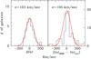 |
Fig. 1 Left-hand panel: distribution of our measured velocity error. Right-hand panel: comparison between our measured radial velocities and those from the SDSS: the agreement between the two data sets is very good within the errors. |
2.2. Redshift measurement
The technique is similar to the one used in Paper I, and again we briefly mention the points that are most important to understand the current data set.
The IRAF2 packages xcsao and emsao were used to measure the galaxy redshifts by means of a cross-correlation method (Tonry & Davis 1979), where robust measurements were obtained for galaxy spectra dominated by either emission lines or absorption lines. For spectra dominated by absorption lines, we used galaxy templates and stellar radial velocity standards, while for emission-line dominated spectra we used a synthetic template generated by the IRAF package linespec. Starting from a list of the stronger emission lines (Hβ, [OIII], [OI], Hα, [NII], [SII]), the package creates a synthetic spectrum, which was then convolved with the instrumental resolution.
A confidence parameter (see Kurtz & Mink 1998, for a complete discussion) was used to assess the goodness of the estimated redshift: all redshifts with a confidence parameter r ≥ 5 were considered reliable, while measurements with 2.5 ≤ r ≤ 5 were checked by hand. Measurements with r ≤ 2.5 are not reliable. All the confirmed member galaxies in our sample had a r > 3.5.
In some cases, emsao failed to correctly identify the emission lines, which happened each time some emission lines were contaminated by underlying absorption. When this occurred, we measured the redshift by Gaussian fitting the strongest emission lines visible and took the average of the results obtained from each line. If two or more lines were blended, the IRAF command deblend within the splot package was used.
The recession velocity errors varied between 15 and 100 km s-1, depending on the kind of the galaxy spectrum (emission or absorption dominated) and also the S/N of the target spectrum.
Corrections to produce heliocentric recession velocities were estimated using the IRAF task rvcorrect in the package noao.rv.
Whenever possible, we checked the existing literature for other published redshifts; in particular, we made extensive use of the overlapping area with the SDSS, SDSS-R7 (see Abazajian et al. 2009). For galaxies that were well separated from other objects, we found a remarkable agreement with exisiting measurements within our measurements errors (see Fig. 1).
Some disagreements were found instead for galaxies close on the sky to either nearby stars or other galaxies with different redshifts. We assumed that this happened mostly because of the fiber proximity limit, which prohibited the Sloan spectrograph from observing targets closer to each other on the sky than 60″ at z = 0.1 in a single pass. We note that when the only available redshifts were photometric, these frequently disagreed with our own spectroscopic measurements.
2.3. Luminosity measurements
We briefly summarize here how we estimated the luminosity of each member galaxy; for a full description, the reader can consult Paper I. The luminosity of each group was obtained by summing up all the luminosities of the member galaxies, after correction for Galactic extinction and k-correction. Only two values of k correction were used, one for early-type galaxies (E-Sa), and another for late-type ones (Sb onward), identified by an EW(Hα) > 6 Å3 and morphological evidence, i.e. presence of spiral arms. No correction for passive evolution was applied, both because not all galaxies in our sample can be characterized by a simple stellar population and owing to the large rms which is comparable at z = 0.1 to the amount of correction that would be applied, assuming the models from van Dokkum et al. Nos. 1, 2, and 3 (Longair 2008). All R band luminosities were converted to B band luminosity using the transformation (Windhorst et al. 1991) based on the empirical relations of Kent (1985):  (1)and assuming that MB,⊙ = 5.48.
Errors in the luminosity were estimated by assuming the maximum error in the photometric calibration of DPOSS plates, i.e. an error of 0.19 mag for an r magnitude of 19 (Gal et al. 2004).
3. Results
This section is divided into two parts. The first part will describe our so-called sample cleaning, i.e. an analysis of the environment surrounding the spectroscopically confirmed groups, to determine whether they fulfil the isolation criteria. This basically divides the confirmed groups into two categories: (1) the objects really isolated on the sky, which can be assumed to be bona fide compact groups; and; (2) objects close on the sky to larger scale structure, to whom they may be associated, or objects that are part of a cluster of galaxies and have been selected as candidate CGs by mistake.
In the second part of this section, we calculate the so-called characteristic parameters of the CGs, namely velocity dispersion, crossing time, radius, and mass, using various estimators, and we compare our measurements with other existing works and with the values of the same parameters obtained for compact groups in the nearby universe.
3.1. Group membership and environment
We consider a candidate compact group to be spectroscopically confirmed if at least three of its members have accordant redshifts, i.e. are within ±1000 km s-1 of the median redshift of the group. The redshift of the confirmed group is assumed to be the median value of the measured redshift of its confirmed members.
To calculate the median group velocity and its radial velocity dispersion, we used the biweight estimators of location and scale (Beers et al. 1990). Among 138 candidate groups, we confirmed 96 concordant objects, i.e. ~70% success rate.
Our measured recession velocities, cz, range from 13 263 km s-1 to 67 724 km s-1 with an average value of 34 792 km s-1, i.e. z = 0.116, one order of magnitude larger than the average value for nearby compact group catalogues. The velocity distribution of our confirmed compact groups is shown in Fig. 2.
We then proceeded to search the environment surrounding each group using available catalogues from the literature and the last SDSS release, and adopting a search radius equal to the Abell radius of a cluster at the distance of each redshifted compact group.
Whenever redshift measurements were available for the literature catalogues used in our investigation of the environment, we refined our search, by assuming that the group is close to a cluster with which it may be associated, if the redshift difference between the two was Δz < 0.01, i.e. a velocity difference of 3000 km s-1, one order of magnitude above the typical velocity dispersion of compact groups.
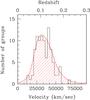 |
Fig. 2 Velocity distribution of our confirmed compact groups. |
This resulted in 62 isolated compact groups and 34 candidate compact groups in the vicinity of a cluster or identified with the cluster core itself. The isolated spectroscopically confirmed groups were labelled class A, while the others were put in class B. To class C belong all candidate CGs with fewer than three concordant members; we note that the majority of class C groups are composed by couples of pairs.
3.2. The small-scale environment
After distinguishing isolated CGs from those close on the sky to larger-scale structure, we proceeded to a closer examination of the environment surrounding our isolated groups. Using again the last release of the SDSS (DR7), and other literature sources, as available from NED, we searched for nearby galaxies within a radius equal to three times the average group radius, RG, (see Sect. 3.6), then a radius equal to 250 kpc, i.e. five times the average group radius and finally a radius equal to 500 kpc, i.e. ten times the average group radius. To ensure that we did not assign random field galaxies to groups, we also checked the radial velocity distribution of the original group members and the newly detected galaxies. A new object was considered an additional member only if its velocity difference from the median velocity of the group is smaller than 1000 km s-1.
The goal of this exercise was to investigate how many of our isolated CGs are part of a wider galaxy distribution and how many are real isolated CGs with a high density on the sky. We must point out that only part of our sample (see Fig. 3) falls within the area covered by the SDSS spectroscopic survey, and that the spectroscopic limit of the SDSS is reached at a magnitude rpetro is 17.7. This means that we do not include in our search all those galaxies whose magnitude is fainter than the spectroscopic limit of SDSS, including potential additional group members whose magnitude ranges from r = 17.8 to r = 19.0, which is, by construction, the fainter magnitude limit of our search for group members. In addition to this, three of our confirmed groups are completely outside the surveyed areas, while another 13 objects are located at the edge of the area covered by the survey.
Despite these limitations, we were able to place constraints on the local environment of almost all our confirmed groups, using also other sources of information available from the literature.
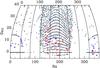 |
Fig. 3 Distribution of our confirmed compact groups over the SDSS spectroscopic coverage. Crosses represent DPOSS CGs within the SDSS spectroscopic coverage, while asterisks are objects located at the edge of a plate or completely outside the surveyed area. |
The results of this search can be resumed as follows:
-
six groups belonging to B class are located at the edge of alarger-scale structure. From our data, it is impossible todetermine whether these groups are interacting with the cluster,but it would be worthwhile to perform spectroscopic follow-upobservations;
-
the remaining B class groups, with the exception of two groups, are either within an Abell cluster or coincide with one of the massive clusters identified by Koester et al. (2007). The last two objects, which are outside the SDSS area coverage on the sky, are associated with an X-ray cluster;
-
groups of class A are a mixed bag of objects: among the total of 62 spectroscopically confirmed groups, we found 12 with unusually large radial velocity dispersions, larger than 400 km s-1, which is more typical of large groups or poor clusters. We discuss these 12 objects in more detail below.
PCG093220+171954 is composed of four galaxies. Looking at the velocity distribution, this group is clearly composed of two pairs of galaxies at similar redshift, surrounded by other galaxies. PCG094321+122625 has a chain-like geometry, i.e. all member galaxies are aligned with each other on the sky. However the redshift distribution of its member galaxies is clearly binomial, revealing this group as a couple of pairs close to each other on the sky. A similar situation, albeit with a different geometry, happens for PCG095527+034508 and PCG153046+123131, i.e. all of them are composed of two close pairs at similar redshift. These two pairs may merge with each other in the future, forming a new group of galaxies, but here these groups were discarded from the final sample. PCG100644+112806 and PCG155341+103913 appear instead to consist of a pair of galaxies with an infalling galaxy, which is quite distant from the other two in velocity space, albeit still within the 1000 km s-1 limit. These objects, which passed the first selection thanks to the small velocity difference between the two pairs, or between the couple and the third galaxy, were excluded from the sample.
PCG121738+121833 and PCG151057+031443 are part of a larger structure on the sky: other galaxies, of magnitude comparable to that of the brighest group galaxy, surround the original members. These are within wider structures of the order of 1 Mpc wide. We define this type of group a loose group.
In addition PCG161009+201350, PCG221442+012823 and PCG225807+011101 are surrounded by other nearby galaxies, but the original members are closer to each other on the sky than the surrounding members. This kind of association is often classified as a loose group, but we call it a core+halo group, following Ribeiro et al. (1998).
It is likely that our selection algorithm selected this kind of structure because the original four members were somehow closer together on the sky than the other galaxies belonging to the structure, triggering a positive detection.
No companions can be found for PCG222633+051207, despite many galaxies being identified in the field, hence it retains its original classification of compact group. However, many bright galaxies are detected in the acquisition images, implying that the environment surrounding this group is a markedly rich one. We then decided to flag this group as suspect and more likely to be a loose group.
Another candidate compact group that was not observed by us, but identified using SDSS data, PCG130257+053112, also contains other four galaxies within 500 kpc and Δ ≤ 1000 km s-1, and was classified as a core+halo group, despite its small velocity dispersion.
This means that from the original 62 isolated and spectroscopically confirmed compact groups, we lose 6, because either close couples or pairs with a third close member, and another 7 are larger-scale structures, i.e. loose or core+halo groups, leaving us with 49 class A, bona fide compact groups.
3.3. Group density on the sky
To ensure that our confirmed groups are really dense concentration of galaxies on the sky, we apply a density criterion, according to the formula (Ribeiro et al. 1998)  (2)where N is the number of galaxies in the group that are spectroscopically confirmed and R is the group radius in Mpc. A compact group is considered such when its galaxy density is equal to or above 103 galaxies Mpc-3. The total distribution of the measured group densities is shown in Fig. 4, which compares the full confirmed group sample with the isolated one and shows the cut-off line at 103 galaxies Mpc-3.
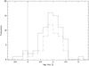 |
Fig. 4 Distribution of the group galaxy density for the whole sample (continuous line) and the class A sample (dotted-dash line). The vertical line is the cut-off density limit at 103 galaxies Mpc-3. The average density is 1.2 × 10⁴ galaxies Mpc-3. |
The density criterion is failed by two class A CGs, PCG093310+092639 and PCG130926+155358, both have small velocity dispersions and very sparse configurations on the sky: these have been discarded from the final sample. This leaves us with only 47 CGs in class A.
If we examine the class B groups, we find that three of them, PCG101113+084127, PCG121346+072712, and PCG151329+025509 have a density below the limit set for CGs: all are in the middle of larger structures, hence we may question how this density would change if the whole larger-scale structure were taken into account.
A special case however is PCG151329+025509, which is in a very perturbed area with another three nearby interacting galaxies: it is at the same redshift as the cluster MaxBCG J228.37839+02.91616 (Koester et al. 2007), and it is unclear whether this is a distant cluster with substructures.
3.4. The final sample of compact groups
Our final candidate CGs classification is then as follows: all the compact group candidates that are not close on the sky to a larger-scale structucture, and fulfil the density criterion are classified as class A. Within this class, three categories of objects are identified:
-
a
real compact groups: 47 final confirmed targets;
-
b
loose groups: 3 objects;
-
c
core+halo groups: 4 objects;
-
d
close couple of pairs or a close pair with a third galaxy within the Δv < 1000 km s-1 limit: 6 objects.
As already mentioned in Sect. 3.2, objects belonging to the last category were removed from the final list. We also excluded loose, core+halo groups, and those groups failing the density criterion from the final list, considering as bona fide compact groups only those at point a .
Candidate compact groups that are close on the sky to a large-scale structure and fulfill the density criterion are classified class B and represent 25% of the whole sample. Within this class, two subcategories are identified:
-
groups that are affected by the larger-scale structure, as traced byan larger than normal velocity dispersion, higher virial mass;
-
groups that, despite their closeness to a larger structure, seem to retain their identity and have velocity dispersion, radius, and mass typical of compact groups. It is likely that these groups will interact with the other structures in the distant future, but at the moment they can be considered as independent structures.
If we consider only class A objects as real compact groups, the success rate of this survey is 34%. The whole sample of observed and confirmed compact groups, with the classification for each group is listed in Table 1.
3.5. Internal dynamics and mass estimates
To understand how our distant CGs, be them isolated or closer to a large-scale structure, compare with nearby ones, we proceed to measure the characteristic properties, i.e. the three-dimensional (3D) velocity dispersion, crossing time, and mass, mass-to-light ratio, using the luminosities derived as explained in Sect. 2.3.
For the 3D velocity dispersion, we use the same equation used in Hickson et al. (1992), the crossing time being defined as:  (3)where R is the median of galaxy-galaxy separations and σ3D is the 3D velocity dispersion. The dimensionless crossing time, shown in Col. 5 of Table 2, Hotc, spans from 0.002 to 0.135, with a median value of 0.020, which is slightly larger than the value measured for HCGs, 0.016.
The median observed velocity dispersion is 273 km s-1, while the 3D velocity dispersion is 382 km s-1, substantially larger than that found for the HCGs (Hickson et al. 1992).
If we restrict ourselves only to isolated groups, i.e. the class A ones, the median crossing time becomes Hotc = 0.024, 50% longer than the crossing time measured for HCGs but still half of the median value measured for SCGs, 0.051. The median radial velocity dispersion is σr = 188 km s-1, while the 3D velocity dispersion is σ3D = 250 km s-1, very similar to that found for nearby CGs.
If we consider the groups associated to larger structures, excluding those in the middle of a cluster, we measure an median radial velocity dispersion of σr = 310 km s-1, while the 3D velocity dispersion is σ3D = 433 km s-1, which is about 1.6 times larger than the value measured for the isolated groups, in agreement with the result of Einasto et al. for loose groups closer to large-scale structures on the sky.
A comparison of the crossing time and velocity dispersion of the whole DPOSS sample and the isolated DPOSS compact groups is shown in Fig. 5. A k-s test shows that the two populations are different at a confidence level of 97%.
 |
Fig. 5 Top panel: distribution of the crossing time for the whole DPOSS sample (continuous line) versus the class A groups (dot-dashed line). Bottom panel: same distribution for the radial velocity dispersion. |
For the mass estimate, we use different estimators, the virial and the projected mass. The expression for the virial mass is given in Eq. (4), which is valid only under the assumption of spherical symmetry.  (4)where Rij is the projected separation between galaxies i and j, here assumed to be the median length of the 2D galaxy-galaxy separation vector, corrected for cosmological effects; N is the number of concordant galaxies in the system, and
  is the velocity component along the line of sight of the galaxy i with respect to the centre of mass of the group. As observed by Heisler et al. (1985) and Perea et al. (1990), the use of the virial theorem produces the best mass estimates, provided that there are no interlopers or projection effects. In case one of these two effects is present, the current values should be considered as upper limits to the real mass.
Another good mass estimate is given by the projected mass estimator, which is defined as  (5)where Ri is the projected separation from the centroid of the system, and fP is a numerical factor depending on the distribution of the orbits around the centre of mass of the system.
Assuming a spherically symmetric system for which the Jeans hydrostatic equilibrium applies, we can express fP in an explicit form (Perea et al. 1990). Since we lack information about the orbit eccentricities, we estimate the mass for radial, circular, and isotropic orbits and the corresponding expressions for MP are given in Eqs. (6)–(8) respectively as  where R is the median length of the 2D galaxy-galaxy separation vector.
The results for the four estimators all agree quite well with each other, and the reported value for the mass in Col. 6 of Table 2 is the average of all four estimates. The averaged values have been used for the estimate of the M/L ratio in Col. 8 of Table 2. We note that revised values for some groups from Paper I are published here, to correct a former error in velocity measurements owing to problematic wavelength calibrations.
The group masses vary from 2.67 × 10¹⁰ to 1.34 × 10¹⁴ M⊙, with an average value of ~1.67 × 10¹³M⊙. The M/L ratio varies from 0.38 to 2476, with an average value of 192, which is larger than that reported for HCGs, and similar to that measured for loose groups of galaxies.
If we restrict ourselves to the isolated compact groups, i.e. the class A ones, the average values of mass and mass-to-light ratio are both lower, i.e. M = 6.6 × 10¹² M⊙, and M/LB = 80, which are very similar to the values measured for compact groups in the nearby universe. Groups close to larger-scale structures have an average mass of M = 2.3 × 10¹³ M⊙, and M/LB = 262. The measured mass is ~2.5 times the value measured for isolated groups, once more in agreement with the result found by Einasto et al. (2003).
3.6. Radius distribution
The typical radius measured for compact groups in the nearby universe is of the order of 50 kpc, or less. We measured the group radius, RG, as the median of the galaxy-galaxy separation within the spectroscopically confirmed members of each group. In Fig. 6, we show the histogram of the radius distribution for our whole sample. The peak of the distribution is at 50 kpc, which is quite consistent with the value measured for compact groups. The mean value does not change if only isolated groups are considered. This is expected, because this radius is measured taking into account only the original, spectroscopically confirmed, group members.
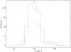 |
Fig. 6 Distribution of the median group radius for the whole DPOSS sample of confirmed compact groups (continous line) and the isolated one (dot-dashed line). |
However, if one computes the virial radius for our objects, as  (9)where ρ200 is 200 times the critical density of the Universe and M is the group virial mass, the average value differs for the whole sample of our confirmed groups and the isolated ones, being R200 = 468 kpc and R200 = 310 kpc, respectively.
3.7. The population of galaxies in the groups
We studied the galaxy morphological types for each group, defining a galaxy to be late type if its Hα equivalent width is larger than 6 Å, following Ribeiro et al. (1998). This choice is motivated by the shallowness of our acquisition images and their varying depth, which do not allow a reliable photometric analysis. This criterion probably allows active galaxies to contaminate the sample; however, the measured fraction of strong AGN (Sy galaxies) in CGs is of the order of 12% (Martinez et al. 2008), and only one galaxy in 238 observed is a broad-line active galaxy. Of 370 galaxies within our group population, we find that 72 are spiral galaxies, i.e. 19% of the total. However, if we subdivide our sample into groups close to a large-scale structure, class B, and isolated groups, class A, the percentage of spiral galaxies changes to 14% and 24%, respectively, i.e. isolated compact groups contain a larger fraction of late-type galaxies.
The spiral fraction is a function of the crossing time as shown in Fig. 7.
The spiral fraction increase can be fit by a linear slope  (10)This trend does not change if only isolated groups are considered, becoming
  (11)The spectroscopic fraction of spiral galaxies is the smallest measured so far in compact groups of galaxies; the number is well below the fraction measured for HCGs, 49%, and for SCGs, 69% (Pompei et al. 2003). Such large difference might be partly caused by our use of a spectroscopic morphological criterion, while the quoted spiral fraction for nearby compact groups was derived from deep photometric studies. However, if only a spectroscopic criterion is used for HCGs, the spiral fraction remains quite high, of the order of 40% (see Fig. 3 of Ribeiro et al. 1998). Hence, it seems that our confirmed compact groups have indeed a smaller fraction of late-type galaxies than HCGs.
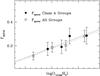 |
Fig. 7 Spectroscopically selected fraction of spiral galaxies as a function of the crossing time for all spectroscopically confirmed groups and for the class A groups only. The solid and dashed lines represent the fits for the class A groups and the whole sample, respectively. |
3.8. Comparison with other surveys
We checked the literature to compare our results with other catalogues of groups of galaxies: since the release of the SDSS DR7, two major catalogues of galaxy groups have been published, one by McConnachie et al. (2009) and another by Tago et al. (2010). We compared our whole observed sample of 138 groups with catalogues A and B from McConnachie and Table 2 from Tago et al. The geometrical center of each group was used in all the catalogues and a search radius of 30″ on the sky was used, returning a total of 23 matches from McConnachie and 5 from Tago et al. The choice of the radius was a compromise between the two different definitions of group center of ourselves and McConnachie, as we both used the geometrical radius, and Tago et al., who used a different method. When redshift measurements were available, a good agreement was found in all cases, except five (see Table 3). In these cases, no more than two redshifts were available from SDSS data, while our own observations proved that the candidate compact group consisted of a couple of pairs at two different redshifts.
Associations between the group catalogue of McConnachie et al. and our confirmed group sample.
The DPOSS cluster catalogue (Lopes et al. 2004) was also searched for possible associations between our candidate CGs and larger-scale structures from the same survey. Here the results were somewhat mixed, because of the disagreement between the quoted photometric redshifts from the DPOSS and our spectroscopic redshifts. Owing to the robustness of the spectroscopic measurements, in particular at such low redshifts, we conclude that our redshift estimates are more reliable and reassign the same distance to the DPOSS cluster that is close on the sky to our candidate DPOSS compact groups and the group itself (see Table 1 for confirmed associations).
4. Discussion
From our analysis, it becomes clear that our original sample of candidate CGs consists of a mixed bag of objects, a significant part of which is embedded in a large-scale structure. Most of the rejected candidates are formed by two pairs of galaxies close together on the sky. Hence, a first result is that finding compact groups at intermediate redshift is not a trivial business, even when using search criteria based on the original Hickson ones and modified to take into account the larger distance. Once the candidate groups have been identified, it is of crucial importance not only to confirm spectroscopically all the candidate member galaxies, but also to study in detail the surrounding environment of the confirmed groups, to have a good understanding of what kind of objects are being observed. This should return a reasonably clean sample of isolated compact groups. Even with these precautions, our final sample represents an upper limit to the amount of isolated compact groups, partially because of the incomplete coverage of the SDSS in the areas observed by ourselves and partially because of the limited spectroscopic coverage for objects fainter than rpetro = 17.7. Despite all these limitations, we have found a fraction of confirmed isolated groups of 34% of the total number of groups originally observed, which is larger than the fraction measured for a subsample of HCGs (de Carvalho et al. 1994, 23%). We wonder, however, what the real fraction for HCGs would have been if the whole 92 confirmed groups catalogue had been studied by de Carvalho et al. (1994).
Our confirmed isolated CGs have an median crossing time equal to about one tenth of the light travel time to us. Assuming the crossing time as an estimate of the group age, we conclude that we do not observe at higher redshift the same population of groups as we observe in the nearby universe; that is we must be looking at a different population of compact groups. If we were to assume that all these groups will continue to exist in isolation without further perturbation from the external environment, the most likely final product of such groups would be an isolated early-type galaxy. According to the model of Barnes (1989), isolated CGs are likely to evolve into a single isolated elliptical galaxies in a few crossing times, hence we expect these z = 0.1 objects to be the progenitors of present-day ellpticals.
To determine whether this conclusion is realistic, at least in qualitative terms, we compared the volume density of our confirmed CGs to the volume density of isolated early-type galaxies drawn from several literature works in the nearby universe. We assumed that the density distribution of our compact groups in space is uniform across the surveyed area, and that our sample is complete all the way to our average redshift; we were then able to estimate an average volume density of CGs based on Eq. (1) of Lee et al. (2004). Our isolated compact groups have a density of 1 × 10⁻⁶ Mpc-3, similar to the values measured for clusters of galaxies (Bramel et al. 2000) and fossil groups (Santos et al. 2007; Jones et al. 2003).
Assuming that the percentage of early-type galaxies is ~18% of all field galaxies (starting from an estimated 82% fraction of spirals in the field, as quoted by Nilson et al. 1973 and Gisler et al. 1980), we applied the same Eq. (1) to the samples of Allam et al. 2005; Giuricin et al. (2000) and AMIGA (Verley et al. 2007). Assuming as an average redshift for each survey the one quoted in each paper, we found that the volume density of early-type galaxies is of the order of a few × 10-5 Mpc-3. If we adopted the maximum redshift of each survey for which completeness is claimed, the number goes down to a few × 10-6 Mpc-3.
We conclude from these numbers that it is perfectly plausible that all our isolated compact groups will end up as early-type galaxies in the field with no overpopulation problem.
Other indirect evidence can further strenghten our reasoning: likely candidates for such end-product from groups were previously observed by the MUSYC-YALE survey (van Dokkum et al. 2005). They are isolated red and dead galaxies, which, on deeper inspection, contain extended tidal tails and shells composed mainly of stars, with a small amount of residual gas, the so-called dry mergers.
If we examine exisisting spectroscopic studies on galaxies in CGs, we find that observations of nearby isolated early-type galaxies (Collobert et al. 2006) have shown that the most massive galaxies in low density environments have abundance ratios similar to those of cluster galaxies. Mendes de Oliveira et al. (2005) also demonstrated that early type galaxies in HCGs are generally old. On the other hand, early-type galaxies in the field with small central velocity dispersions have properties that are consistent with extended episodes of star formation (Collobert et al. 2006), as if coming from a past of multiple interaction and slow buildup.
Available X-ray observations of CGs reveal a wide range of the X-ray diffuse emission, with a slight tendency for spiral-rich groups to have a small amount of X-ray emission (Ponman et al. 1996). An opposite trend is tentatively detected for the HI content (Verdes-Montenegro et al. 2001; Pompei et al. 2007).
On the basis of these observations, the following scenario can be envisioned: galaxies belonging to more massive CGs evolve mainly within the group environment, giving rise to either a fossil group, i.e. a massive elliptical galaxy, surrounded by several dwarf galaxies, or to a field elliptical, whose abundance ratios are similar to those observed in clusters. As the galaxies have already evolved within the group, no or very little young stellar population should be present and they should continue to evolve via dry mergers. In both cases, the aforementioned X-ray emission is expected.
Galaxies belonging to less massive compact groups evolve in a more gradual way, probably by means of stripping of gas from each other through harassment, giving rise to several episodes of nuclear star formation, and diffuse HI emission within the group potential. They will likely end up as a single isolated early-type galaxy with a younger stellar population than those observed in clusters of galaxies and possibly extended tidal features composed of a small percentage of gas and a high percentage of stars, which are the mute witnesses of the final merger of the compact group in a single galaxy. No or very little X-ray emission is expected in this case, because almost all the existing gas would have been either exhausted in the former episodes of star formation or lost into the intergalactic medium. The dominant factors in shaping the different evolutionary pattern seem to be the velocity dispersion of the group and its initial mass.
Moving toward the class B groups, we find that among 34, nine groups are close to larger-scale structures but not embedded within them; four of these groups have characteristics that are very similar to isolated compact groups, while the others are likely to be affected by the cluster potential, as deduced from their larger velocity dispersion and group position with respect to the cluster.
The percentage of DPOSS groups closer on the sky to larger-scale structures is 25% (34 over 96 confirmed groups), in agreement with what has been found by Andernach & Coziol (2005). The higher mass and larger velocity dispersion of groups in the proximity of larger scale structures support the findings of Einasto et al., of the hierarchical formation of galaxies. In this scenario, it can be postulated than less massive groups formed in lower density regions of the cosmic filaments.
5. Conclusions
We have presented our results of a spectroscopic survey of compact groups at a median redshift of z ~ = 0.12, i.e. a factor of ten larger than any previous study. These can be summerized as follows:
-
Among a total of 138 observed groups, we confirm96 compact groups with 3 or more accordant members.
-
Forty-seven of the confirmed groups are isolated groups on the sky, i.e. a success rate of 34%.
-
The average mass, mass-to-light ratio, crossing time, radius, and velocity dispersion of our isolated compact groups are very similar to the values obtained for compact groups in the nearby Universe. These values are different from those measured for groups close to a larger-scale structure on the sky.
-
Isolated compact groups tend to have a longer crossing time and a higher fraction of spiral galaxies.
-
The volume density of isolated compact groups is consistent with the hypothesis that all of them will conclude their life as a single isolated early-type galaxy. Depending on the original mass and velocity dispersion of the group, we expect the final merger product to resemble a cluster or a field galaxy, with or without an extended X-ray halo.
-
Nine confirmed groups are larger-scale structures, loose groups, or core+halo groups, and will likely behave differently from an isolated compact group.
-
Six objects were discarded, because they were close couples of pairs in redshift space and during the first selection were mistaken for compact groups. It is possible that such close couples of pairs can come together to form a group, but this is at the moment a matter of speculation.
-
Thirty-four of the confirmed groups are close on the sky to a larger-scale structure, to which they might be associated. Of these groups, four are still retaining their identity, while five others are probably already being perturbed by the cluster potential. The percentage of association between groups and larger-scale clusters is in agreement with that found by Andernach & Coziol (2005).
We stress that each study of compact groups or any specific environment, needs careful to incorporate consideration of the surrounding larger-scale, in order to have a clear understanding of the kind of sample one is dealing with.
Online material
List of our observed compact groups, group coordinates, number of member galaxies, average redshift, and our group classification as described in the text.
Group dynamical properties.
Appendix A
We present here a set of figures representative of class A, class B groups.
 |
Fig. A.1 Stacked R band acquisition images for a sample of class A confirmed compact groups. From top left to bottom right, in increasing right ascension order: PCG001108+054449, PCG015254-001033, PCG102512+091835, PCG114233+140738, PCG151833-013726, and PCG235439+032308. The black lines visible in some images are the gap between the two CCDs on the EMMI red mosaic. In all cases the whole group was in one chip, but imaged at different rotation angles, to position accurately the slit. Exposure times vary from 180 s to 450 s. In all images N is up and E is left. |
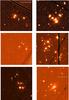 |
Fig. A.2 Same for Fig. 8, but for class B groups. From top left to bottom right, in increasing right ascension order: PCG031139+072404, PCG091524+213038, PCG105400+113327, PCG111250+132815, PCG151037+061618, and PCG234100+000450. |
Acknowledgments
Sincere thanks go to the glorious La Silla Science Operations Team from 2004 to 2008, among them: Ivo Saviane, Gaspare Lo Curto, Valentin Ivanov, Julia Scharwaecther, Jorge Miranda, Karla Aubel, Duncan Castex, Manuel Pizarro, Monica Castillo, and Ariel Sanchez without whom none of these data would have been acquired and without whose company, patience, and fun none of these data would have gone into publication. Special thanks also to the NED team, for the impressive database and for their prompt and professional answers to email queries. E.P. wishes to acknowledge the ESO Director General Discretionary Fund (DGDF) program for two visits at Milan Observatory and INAF for an extended visit to Milan Brera Observatory in 2011, which allowed the completion of this paper.
References
- Abazajian, N. K., & the SDSS team 2009, ApJS, 182, 543 [NASA ADS] [CrossRef] [Google Scholar]
- Allam, S. S., Tucker, D. L., & Allyn Smyth, J. 2005, AJ, 129, 5 [Google Scholar]
- Andernach, H., & Coziol, R. 2005, ASP, 329, 67 [NASA ADS] [Google Scholar]
- Andersen, J., Nordstrom, B., Ardeberg, A., et al. 1985, A&AS, 59, 15 [NASA ADS] [Google Scholar]
- Barnes, J. E. 1989, Nature, 338, 123 [NASA ADS] [CrossRef] [Google Scholar]
- Beers, T., Flynn, K., & Gebhardt, K. 1990 AJ, 100, 32 [Google Scholar]
- Bramel, D. A., Nichol, R. C., & Pope, A. C. 2000, ApJ, 533, 601 [NASA ADS] [CrossRef] [Google Scholar]
- Colber, J. W., Mulchaey, J. S., & Zabludoff, A. 2001, AJ, 121, 808 [NASA ADS] [CrossRef] [Google Scholar]
- Collobert, M., Sarzi, M., Davies, R. L., Kuntschner, H., & Colless, M. 2006, MNRAS, 370, 1213 [NASA ADS] [CrossRef] [Google Scholar]
- de Carvalho, R. R., Ribeiro, A., & Zepf, S. 1994, ApJS, 93, 47 [NASA ADS] [CrossRef] [Google Scholar]
- de Carvalho, R. R., Goncalves, T. S., Iovino, A., et al. 2005, AJ, 130, 425 [NASA ADS] [CrossRef] [Google Scholar]
- Einasto, M., Einasto, J., Mueller, V., Heinamaki, P., & Tucker, D. L. 2003, A&A, 401, 851 [NASA ADS] [CrossRef] [EDP Sciences] [Google Scholar]
- Gal, R. R., de Carvalho, R. R., Odewahn, S. C., et al. 2004, AJ, 128, 3082 [NASA ADS] [CrossRef] [Google Scholar]
- Gisler, G. R. 1980, AJ, 85, 623 [NASA ADS] [CrossRef] [Google Scholar]
- Giuricin, G., Marinoni, C., Ceriani, L., & Pisani, A. 2000, ApJ, 543, 178 [NASA ADS] [CrossRef] [Google Scholar]
- Gutierrez, C. M. 2011, ApJ, 737, L21 [NASA ADS] [CrossRef] [Google Scholar]
- Heisler, J., Tremaine, S., & Bahcall, J. 1985, ApJ, 298, 8 [NASA ADS] [CrossRef] [Google Scholar]
- Hickson, P. 1982, ApJ, 255, 382 [NASA ADS] [CrossRef] [Google Scholar]
- Hickson, P., Mendes de Oliveira, C., Huchra, J. P., & Palumbo, G. G. C. 1992, ApJ, 399, 353 [NASA ADS] [CrossRef] [EDP Sciences] [MathSciNet] [PubMed] [Google Scholar]
- Iovino, A., de Carvalho, R. R., Gal, R. R., et al. 2003, AJ, 125, 1660 [NASA ADS] [CrossRef] [Google Scholar]
- Jones, L. R., Ponman, T. J., Horton, A., et al. 2003, MNRAS, 343, 627 [NASA ADS] [CrossRef] [Google Scholar]
- Kent, S. M. 1985, PASP, 97, 165 [NASA ADS] [CrossRef] [Google Scholar]
- Koester, B. P., McKay, T. A., Annis, J., et al. 2007, ApJ, 660, 239 [NASA ADS] [CrossRef] [Google Scholar]
- Kurtz, M. J., & Mink, D. J. 1998, PASP, 110, 934 [NASA ADS] [CrossRef] [Google Scholar]
- Lee, B. C., Allam, S. S., Tucker, D. L., et al. 2004, AJ, 127, 1811 [NASA ADS] [CrossRef] [Google Scholar]
- Longair, M. S. 2008, Galaxy formation, A&A library (Springer Verlag) [Google Scholar]
- Lopes, P. A. A., de Carvalho, R. R., Gal, R. R., et al. 2004, AJ, 128, 1017 [NASA ADS] [CrossRef] [Google Scholar]
- Martinez, M. A., Del Olmo, A., Coziol, R., & Focardi, P. 2008, ApJ, 678, L9 [NASA ADS] [CrossRef] [Google Scholar]
- Mendes de Oliveira, C., & Hickson, P. 1994, ApJ, 427, 684 [NASA ADS] [CrossRef] [Google Scholar]
- Mendes de Oliveira, C., Coelho, P., Gonzalez, J. J., & Barbuy, B. 2005, AJ, 130, 55 [NASA ADS] [CrossRef] [Google Scholar]
- McConnachie, A. W., Patton, D. R., Ellison, S. L., & Simard, L. 2009, MNRAS, 395, 255 [NASA ADS] [CrossRef] [Google Scholar]
- Nilson, P. 1973, Uppsala general catalogue of galaxies, Uppsala: Astronomiska Observatorium [Google Scholar]
- Perea, J., del Olmo, A., & Moles, M. 1990, A&A, 237, 319 [NASA ADS] [Google Scholar]
- Pompei, E., & Iovino, A. 2003, Ap&SS, 285, 133 [NASA ADS] [CrossRef] [Google Scholar]
- Pompei, E., de Carvalho, R. R., & Iovino, A. 2006, A&A, 445, 857 (Paper I) [NASA ADS] [CrossRef] [EDP Sciences] [Google Scholar]
- Pompei, E., Dahlem, M., & Iovino, A. 2007, A&A, 473, 399 [NASA ADS] [CrossRef] [EDP Sciences] [Google Scholar]
- Ponman, T. J., Bourner, P. D. J., Ebeling, H., & Bohringer, H. 1996, MNRAS, 283, 690 [NASA ADS] [CrossRef] [Google Scholar]
- Ribeiro, A., de Carvalho, R. R., Capelato, H., & Zepf, S. E. 1998, ApJ, 497, 72 [NASA ADS] [CrossRef] [Google Scholar]
- Santos, W. A., Mendes de Oliveira, C., & Laerte Sodre, Jr. 2007, AJ, 134, 1551 [NASA ADS] [CrossRef] [Google Scholar]
- Tago, E., Saar, E., Tempel, E., et al. 2010, A&A, 514, A102 [NASA ADS] [CrossRef] [EDP Sciences] [Google Scholar]
- Tonry, J., & Davis, M. 1979, AJ, 84, 1511 [NASA ADS] [CrossRef] [Google Scholar]
- van Dokkum, P. 2005, AJ, 130, 2647 [NASA ADS] [CrossRef] [Google Scholar]
- Verdes-Mentenegro, L., Yun, M. S., Williams, B. A., et al. 2001, A&A, 377, 812 [NASA ADS] [CrossRef] [EDP Sciences] [Google Scholar]
- Verley, S., Odewahn, S. C., Verdes-Montenegro, L., et al. 2007, A&A, 470, 505 [NASA ADS] [CrossRef] [EDP Sciences] [Google Scholar]
- West, M. 1989, ApJ, 344, 535 [NASA ADS] [CrossRef] [Google Scholar]
- Windhorst, R. A., Burstein, D., Mathis, D. F., et al. 1991, ApJ, 380, 362 [NASA ADS] [CrossRef] [Google Scholar]
All Tables
Associations between the group catalogue of McConnachie et al. and our confirmed group sample.
List of our observed compact groups, group coordinates, number of member galaxies, average redshift, and our group classification as described in the text.
All Figures
|
Fig. 1 Left-hand panel: distribution of our measured velocity error. Right-hand panel: comparison between our measured radial velocities and those from the SDSS: the agreement between the two data sets is very good within the errors. |
| In the text | |
|
Fig. 2 Velocity distribution of our confirmed compact groups. |
| In the text | |
|
Fig. 3 Distribution of our confirmed compact groups over the SDSS spectroscopic coverage. Crosses represent DPOSS CGs within the SDSS spectroscopic coverage, while asterisks are objects located at the edge of a plate or completely outside the surveyed area. |
| In the text | |
|
Fig. 4 Distribution of the group galaxy density for the whole sample (continuous line) and the class A sample (dotted-dash line). The vertical line is the cut-off density limit at 103 galaxies Mpc-3. The average density is 1.2 × 10⁴ galaxies Mpc-3. |
| In the text | |
|
Fig. 5 Top panel: distribution of the crossing time for the whole DPOSS sample (continuous line) versus the class A groups (dot-dashed line). Bottom panel: same distribution for the radial velocity dispersion. |
| In the text | |
|
Fig. 6 Distribution of the median group radius for the whole DPOSS sample of confirmed compact groups (continous line) and the isolated one (dot-dashed line). |
| In the text | |
|
Fig. 7 Spectroscopically selected fraction of spiral galaxies as a function of the crossing time for all spectroscopically confirmed groups and for the class A groups only. The solid and dashed lines represent the fits for the class A groups and the whole sample, respectively. |
| In the text | |
|
Fig. A.1 Stacked R band acquisition images for a sample of class A confirmed compact groups. From top left to bottom right, in increasing right ascension order: PCG001108+054449, PCG015254-001033, PCG102512+091835, PCG114233+140738, PCG151833-013726, and PCG235439+032308. The black lines visible in some images are the gap between the two CCDs on the EMMI red mosaic. In all cases the whole group was in one chip, but imaged at different rotation angles, to position accurately the slit. Exposure times vary from 180 s to 450 s. In all images N is up and E is left. |
| In the text | |
|
Fig. A.2 Same for Fig. 8, but for class B groups. From top left to bottom right, in increasing right ascension order: PCG031139+072404, PCG091524+213038, PCG105400+113327, PCG111250+132815, PCG151037+061618, and PCG234100+000450. |
| In the text | |
Current usage metrics show cumulative count of Article Views (full-text article views including HTML views, PDF and ePub downloads, according to the available data) and Abstracts Views on Vision4Press platform.
Data correspond to usage on the plateform after 2015. The current usage metrics is available 48-96 hours after online publication and is updated daily on week days.
Initial download of the metrics may take a while.