| Issue |
A&A
Volume 539, March 2012
|
|
|---|---|---|
| Article Number | A63 | |
| Number of page(s) | 18 | |
| Section | Stellar structure and evolution | |
| DOI | https://doi.org/10.1051/0004-6361/201118156 | |
| Published online | 24 February 2012 | |
Estimating stellar mean density through seismic inversions
1 LESIA – Observatoire de Paris, CNRS, UPMC Univ. Paris 06, Univ. Paris-Diderot, 5 place Jules Janssen, 92195 Meudon, France
2 Institut d’Astrophysique et Géophysique de l’Université de Liège, Allée du 6 août 17, 4000 Liège, Belgium
e-mail: This email address is being protected from spambots. You need JavaScript enabled to view it.
3 Georg-August-Universität Göttingen, Institut für Astrophysik, 37077 Göttingen, Germany
4 High Altitude Observatory, National Center for Atmospheric Research, Boulder, CO 80307, USA
5 The School of Mathematics and Statistics, University of Sheffield, Hicks Building, Hounsfield Road, S3 7RH, Sheffield, UK
6 Department of Astronomy, Yale University, PO Box 208101, New Haven, CT 06520-8101, USA
Received: 26 September 2011
Accepted: 4 January 2012
Abstract
Context. Determining the mass of stars is crucial both for improving stellar evolution theory and for characterising exoplanetary systems. Asteroseismology offers a promising way for estimating the stellar mean density. When combined with accurate radii determinations, such as are expected from Gaia, this yields accurate stellar masses. The main difficulty is finding the best way to extract the mean density of a star from a set of observed frequencies.
Aims. We seek to establish a new method for estimating the stellar mean density, which combines the simplicity of a scaling law while providing the accuracy of an inversion technique.
Methods. We provide a framework in which to construct and evaluate kernel-based linear inversions that directly yield the mean density of a star. We then describe three different inversion techniques (SOLA and two scaling laws) and apply them to the Sun, several test cases and three stars, α Cen B, HD 49933 and HD 49385, two of which are observed by CoRoT.
Results. The SOLA (subtractive optimally localised averages) approach and the scaling law based on the surface correcting technique described by Kjeldsen et al. (2008, ApJ, 683, L175) yield comparable results that can reach an accuracy of 0.5% and are better than scaling the large frequency separation. The reason for this is that the averaging kernels from the two first methods are comparable in quality and are better than what is obtained with the large frequency separation. It is also shown that scaling the large frequency separation is more sensitive to near-surface effects, but is much less affected by an incorrect mode identification. As a result, one can identify pulsation modes by looking for an ℓ and n assignment which provides the best agreement between the results from the large frequency separation and those from one of the two other methods. Non-linear effects are also discussed, as is the effects of mixed modes. In particular, we show that mixed modes bring little improvement to the mean density estimates because of their poorly adapted kernels.
Key words: stars: oscillations / stars: fundamental parameters / stars: interiors / asteroseismology / Sun: helioseismology
© ESO, 2012
1. Introduction
Determining accurate stellar mass is crucial to several domains in astrophysics. Indeed, mass plays a dominant role in the evolution and final fate of stars. It is also a key parameter when characterising exoplanetary systems since the masses of exoplanets, essential for determining whether they are rocky or gaseous in nature, are in general determined with respect to that of the star. However, in spite of its importance, stellar mass is usually difficult to obtain accurately for single stars and is frequently model-dependent.
A method which has often been used for estimating stellar mass is to compare the position of a star in an Hertzsprung-Russell (HR) diagram with evolutionary tracks for stellar models of different masses. The main difficulties with this method are its model dependence, the large error bars, and the fact that there are regions in the HR diagram in which more than one stellar evolution track goes through each and every point. A promising alternative is to use asteroseismology. Indeed, acoustic modes are a sensitive indicator of the mean density of a star. Current space missions CoRoT (e.g. Michel et al. 2008) and Kepler (e.g. Kjeldsen et al. 2010) are measuring stellar pulsation frequencies to high accuracy. When combined with an independent determination of the radius, this yields the stellar mass. Thanks to very precise parallax measurements, radii accurate to 2% are expected from the forthcoming astrometric mission Gaia (Perryman et al. 2001). The main challenge is then finding the best way of extracting the mean density of a star from a given set of frequencies.
Various methods have been devised or proposed for estimating stellar mean density from pulsation frequencies. These include using simple scaling laws based on the large frequency separation (Ulrich 1986) or other frequency combinations (Kjeldsen et al. 2008), searching for the best-fitting model within a grid of models or a parameter space and retaining its mean density (e.g. Bazot et al. 2008; Metcalfe et al. 2010; Kallinger et al. 2010), and performing a full structural inversion to determine the density profile, then integrating it to obtain the mean density. The structural inversion may be carried out using linear or non-linear techniques (e.g. Gough & Thompson 1991; Antia 1996; Roxburgh & Vorontsov 2002). The scaling relations have the obvious advantage of simplicity over the other methods and require fewer frequencies than full structural inversions, but are less accurate. Although more expensive computationally, searching for best-fitting models in a grid is also straightforward and usually more precise, but is model-dependent, so that the conclusions are only as firm as the input physics. Full structural inversions have the advantage of being less model-dependent, but usually involve a number of free parameters which need careful adjustment and can fail to converge when non-linear. However, with the current missions CoRoT and Kepler and future asteroseismic projects, there is a growing need to provide accurate seismic stellar masses for a large number of stars in an automatic way. An ideal method would combine the advantages of the above techniques while avoiding their weaknesses.
In this paper, we focus on kernel-based linear inversion methods that directly yield the mean density without inverting for the full density profile. As such, this represents a first attempt at constructing methods which combine the simplicity of scaling laws with the accuracy of full structural inversions. Although the results are not as accurate as initially hoped for, this approach gives insight into the precise relation between the mean density of a star and pulsation modes, and provides a better way of evaluating scaling laws. Section 2 establishes a general framework in which to construct and evaluate linear inversion techniques which yield the mean density directly. The following section then describes various linear inversion techniques, including linearised scaling laws. This is followed by a section which shows how to extend these techniques beyond the linear regime. Sections 5–7 apply these different methods to the Sun, to test cases using a grid of models, and to three stars, two of which were observed by CoRoT (HD 49933 and HD 49385). Finally a discussion concludes the paper.
2. General aspects
2.1. Starting point
As for most inversion methods, the methods described below start with an observed star and a reference stellar model. At this point we will assume that the star and the model have the same radius, but will relax this constraint later on. The structure of the reference model needs to be sufficiently close to the structure of the star so that the link between the relative frequency differences, δνnℓ/νnℓ, and the differences in the stellar structure can be described by a linear relation:  (1)where ρ is the density, Γ1 the first adiabatic exponent, x = r/R the fractional radius, n the radial order, ℓ the harmonic degree, R the radius and
  an ad hoc surface term (e.g. Christensen-Dalsgaard & Berthomieu 1991). The function Fsurf is assumed to be a slowly varying function of ν only, and Qnℓ represents the mode’s inertia (e.g. Aerts et al. 2010), normalised by the inertia of a radial mode, interpolated to the same frequency. The kernels
  and
and  are known functions which can be deduced from the (n,ℓ) eigenmode of the reference model, via the variational principle (Gough & Thompson 1991). Although the above relation can also be applied to other structural pairs, we will work with the pair (ρ,Γ1) since ρ is an obvious choice for finding the mean density, and Γ1 is expected to vary little between different models. Throughout this paper, we will use the following definition for the relative difference of a quantity f, although we note that other definitions have been used (e.g. Antia & Basu 1994):
  (2)With this definition, we have the relation fobs = fref(1 + δf/f).
The mass difference, δM, between the reference model and the star is given by  (3)From this equation it is possible to deduce the relative difference in mean density,
  ,
,  (4)where the quantity ρR = M/R3 is used for non-dimensionalisation. It is important to note that if δρ/ρ ≡ 1 then
  , in other words
  (5)If we now assume that the radius of the reference model is different from that of the star, then the model can be rescaled through homology, i.e. a transformation which preserves all dimensionless quantities, so as to have the same radius as the star. Furthermore, the mean density needs to be kept the same to avoid modifying the pulsation frequencies when rescaling the model. Equation (3) will then give the relative mass difference between the star and the rescaled reference model. However, given their non-dimensional form and because the density is preserved between the original and scaled models, Eqs. (1) and (4) remain unchanged and can be applied directly to the original (unscaled) reference model, as long as x = 1 corresponds to both the radius of the star, and the radius of the reference model. The procedures which will be described below are based on these two equations, and therefore do not require explicitly scaling the reference model to the same radius as the star. They will consequently yield the mean density rather than the mass, although the latter can be deduced if the radius is known.
2.2. Linear inversions
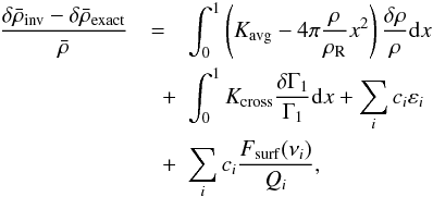
The procedures described in this paper then consist in searching for a linear combination of the relative frequency differences that best reproduces the relative mean density variation,  :
:  (6)where the index i represents the pair (n,ℓ). Using Eq. (1) to replace δνi/νi then yields the following expression:
  (7)where
  In order for
  to be a good estimate of the relative mean density variation, the averaging kernel, Kavg, needs to be as close as possible to 4πx2ρ/ρR, as can be seen by comparing Eqs. (7) and (4). Furthermore, Kcross, which represents the cross-talk coming from relative variations on the Γ1 profile, needs to be reduced as does the last term, which represents the surface effects. Hence, these kernels provide a natural way of evaluating an inversion procedure (e.g. Christensen-Dalsgaard et al. 1990).
2.3. Various error bars
The starting point for obtaining the error on the mean density estimate is to calculate the difference  :
:  (10)where the εi are the actual errors on the relative frequency differences resulting from measurement errors. If the true density and Γ1 profiles are known beforehand (for instance when testing the methods on stellar models rather than true stars) then it is possible to quantify separately the different contributions to the error using Eq. (10). Of course, in a realistic case, such profiles are not accessible.
Using Eq. (10), one can seek an upper bound on the error through the Cauchy-Schwartz inequality: 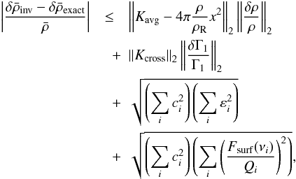 (11)where
 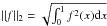 . The difficulty, of course, is finding reasonable estimates for ∥ δρ/ρ ∥ 2, ∥ δΓ1/Γ1 ∥ 2, and
 ![Mathematical equation: \hbox{$\sqrt{\sum_i \left[F_{\mathrm{surf}} (\nu_i)/Q_i\right]^2}$}](/articles/aa/full_html/2012/03/aa18156-11/aa18156-11-eq49.png) . In their solar structural inversions, Rabello-Soares et al. (1999) used the quantity ∥ Kavg − T ∥ 2 as a measure of how well the averaging kernels matched specified target functions, T (which in their case were localised around specific grid points), and ∥ Kcross ∥ 2 to characterise how well cross-talk was being suppressed.
. In their solar structural inversions, Rabello-Soares et al. (1999) used the quantity ∥ Kavg − T ∥ 2 as a measure of how well the averaging kernels matched specified target functions, T (which in their case were localised around specific grid points), and ∥ Kcross ∥ 2 to characterise how well cross-talk was being suppressed.
It is also useful to look at the statistical error on the estimated density variation, resulting from frequency measurement error. Let us denote as σi the 1σ error bar on the relative frequency differences, δνi/νi. The resulting 1σ error bar on the estimated mean density variation is then given by 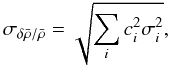 (12)where we have assumed that the errors on the individual frequencies are independent. The quantity
  is known as the error magnification and is the amount by which the error is amplified if the σi are uniform.
It is important to realise that there are other sources of error besides those given in Eq. (10). These include non-linear effects where Eq. (1) is no longer valid, non-adiabatic effects which are not included in the pulsation calculations nor in the variational principle (used to calculate the kernels), inaccuracies in the structural kernels which come from neglecting surface terms in the integration by parts (although these may be absorbed up to some extent in ∑ iciFsurf(νi)/Qi) and numerical inaccuracies.
2.4. Homologous transformations
Before proceding to describe various inversion procedures, it is useful to point out simple properties which can be deduced from homologous transformations. Let us suppose that the observed star can be deduced from the model through a homologous transformation, such that the relative density variation is  , where ϵ is a small quantity. As is well known from dimensional analysis, the frequencies scale with
  . Therefore, to first order the relative frequency variation will be ϵ/2. As a consequence, a necessary and sufficient condition to obtain the correct inversion result in the case of a homologous transformation is
  (13)where we have made use of Eq. (6). In what follows, inversion procedures which satisfy this condition will be called “unbiased”.
Furthermore, one can also deduce a simple property about the Kρ,Γ1 kernels. Remembering that δΓ1/Γ1 = 0 in a homologous transformation and making use of Eq. (1) yields the following result:  (14)This relation is approximate because in deriving the kernel Kρ,Γ1, there are several integrations by part in which surface terms are neglected (Gough & Thompson 1991). Nonetheless, Eq. (14) is satisfied to a good degree of accuracy.
Using Eqs. (14), (8) and (5), it is possible to re-express Eq. (13) as follows:  (15)which is another way of expressing that an inversion procedure is unbiased.
3. Inversion procedures
We will now describe three different methods for estimating the mean density of a star. The first method is an inversion procedure that directly yields inversion coefficients, ci. The next two methods are non-linear scaling laws rather than inversion procedures. In order to put them in the same form as an inversion procedure, we linearise these laws and obtain associated coefficients ci. This then allows a systematic comparison of the three methods using the averaging and cross-term kernels. Hence, although the second and third method are not initially inversion procedures, they will be treated and described as such below.
3.1. SOLA inversion
The SOLA procedure (subtractive optimally localised averages, Pijpers & Thompson 1992, 1994) consists in optimising Kavg by minimising its difference with a specified target function, T, and reducing the effects of the remaining terms. This is achieved by minimising the following cost function: 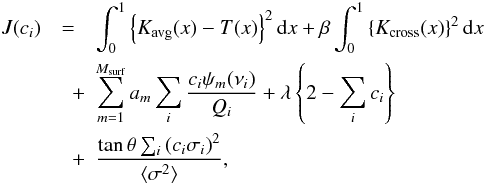 (16)where
  , N being the number of observed frequencies. In order to obtain the relative mean density variation, the appropriate target function is
  (17)The first term on the right-hand side of Eq. (16) is used to reduce the differences between Kavg and T, and the next two terms minimise the effects of cross-talk from Γ1 and pollution from unknown near-surface effects. The functions ψm are a basis of slowly varying functions, such as the first Msurf Legendre polynomials, and the am are Lagrange multipliers, which are used to suppress these terms. The fourth term ensures that the inversion is not biased, λ being a Lagrange multiplier. Finally, the last term is a regularisation term which reduces
  (see Eq. (12)). The free parameters in this approach are β, which regulates between optimising Kavg and minimising Kcross, θ, which is used to adjust the amount of regularisation, and Msurf, which controls the number of terms used in suppressing unknown surface effects.
Using Eq. (17) to define the target function avoids inverting for the entire density variation profile, δρ, and integrating it to obtain the mean density variation, which simplifies the calculations and reduces the number of free parameters (such as the choice of a grid on which to carry out the inversion, or the width of the target functions at each grid point). Furthermore, the averaging and cross-term kernels are calculated for the inverted mean density variation, rather than for the density at specific grid points, which is more useful in evaluating the inversion errors. Finally, it is worth noting that Pijpers (1998) had already used a similar direct approach to determine the Sun’s moment of inertia rather than integrating the rotation profile, and had found similar benefits.
3.2. Large frequency separation
An alternative approach is to use the well-known scaling law between the mean density and the large frequency separation (e.g. Ulrich 1986)  (18)where ⟨ Δν ⟩ is an average of the large frequency separation, νn + 1, ℓ − νn, ℓ. This law has been applied by many authors to obtain the mean density of a variety of stars (e.g. Kjeldsen & Bedding 1995, Mosser et al. 2010). Recently, White et al. (2011) have investigated its accuracy for a grid of models and showed that the error is around 2 to 3.5% for stars with Teff below 6700 K, relevant to solar-like oscillations, but can reach 10% in the worst cases, when calibrated to solar values.
Equation (18) stems from the fact that the frequencies, and consequently any linear combination thereof, also scale with  for homologous transformations, as was pointed out in Sect. 2.4. This still approximately holds for non-homologous transformations, although some dependence on the precise stellar structure will appear. Asymptotic analysis shows that for high-order p-modes,
 ![Mathematical equation: \hbox{$\langle \Delta \nu \rangle = \left[2\int_0^R \frac{{\rm d}r}{c}\right]^{-1}$}](/articles/aa/full_html/2012/03/aa18156-11/aa18156-11-eq90.png) , i.e. the inverse of the time it takes for a sound wave to travel from the surface of a star to its centre and back again (Vandakurov 1967). Given that sound waves travel more slowly near the surface, the large frequency separation is sensitive to surface conditions.
, i.e. the inverse of the time it takes for a sound wave to travel from the surface of a star to its centre and back again (Vandakurov 1967). Given that sound waves travel more slowly near the surface, the large frequency separation is sensitive to surface conditions.
As such, this law is not directly comparable to the above procedure. However, one can apply this law in differential form, i.e. chose a reference model which is close to the star, calibrate the law using this model, and evaluate the mean density of the star. Given that the reference model is close to the star, one can simply perturb Eq. (18) to relate the relative variation of the large frequency separation to the relative mean density variation:  (19)If we assume that the average large frequency separation can be expressed as a linear combination of the frequencies, ⟨ Δν ⟩ = ∑ idiνi, the left-hand side of Eq. (19) becomes
  (20)where
  (21)Equation (19) then takes on the form given in Eq. (6). Consequently, it is also possible to construct averaging and cross-term kernels for this approach, which can then be compared with those coming from the SOLA approach. By construction, this approach is unbiased and will therefore provide the correct answer for homologous transformations. One can also easily verify that ∑ ici = 2.
It is important to realise that although the large frequency separation is typically applied to p-modes in the asymptotic regime, Eqs. (18) and (19) have a more general application. Indeed, what is important is the scaling which applies to all modes, not the fact that the large separation asymptotically gives the inverse sound travel time. Hence, unless specified otherwise, we will typically use all of the available modes when applying Eqs. (18) and (19).
In what follows, we will use the following estimate for the large frequency separation to obtain the coefficients di: 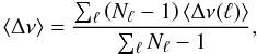 (22)where
 ![Mathematical equation: \begin{eqnarray} \langle \Delta \nu(\l) \rangle &=& \frac{\sum_{i=1}^{N_{\l}} \left[\nu_i(\l) - \langle \nu(\l) \rangle\right] \left[n_i(\l) - \langle n(\l) \rangle\right]} {\sum_{i=1}^{N_{\l}} \left[n_i(\l) - \langle n(\l)\rangle\right]^2}, \\ \langle \nu(\l) \rangle &=& \frac{1}{N_{\l}} \sum_{i=1}^{N_{\l}} \nu_i(\l), \\ \langle n(\l) \rangle &=& \frac{1}{N_{\l}} \sum_{i=1}^{N_{\l}} n_i(\l). \end{eqnarray}](/articles/aa/full_html/2012/03/aa18156-11/aa18156-11-eq98.png) Here, Nℓ is the number of modes with a given harmonic degree, ℓ, and the ni(ℓ) and νi(ℓ) are their associated radial orders and frequencies, respectively. The above definition is a weighted average of the least-squares estimates of the mean large frequency separation from Kjeldsen et al. (2008) for each ℓ value. Using a least-squares approach has the advantage of not requiring consecutive radial orders to estimate the large frequency separation.
Here, Nℓ is the number of modes with a given harmonic degree, ℓ, and the ni(ℓ) and νi(ℓ) are their associated radial orders and frequencies, respectively. The above definition is a weighted average of the least-squares estimates of the mean large frequency separation from Kjeldsen et al. (2008) for each ℓ value. Using a least-squares approach has the advantage of not requiring consecutive radial orders to estimate the large frequency separation.
3.3. The KBCD approach
Recently, Kjeldsen et al. (2008) proposed a method for correcting unknown surface effects which they treated as a power law. This method uses a combination of the large frequency separation and an average of the frequencies to estimate either the exponent of the power law or the mean density of the star. Having established the value of the exponent in the solar case, Kjeldsen et al. (2008) then go on to use this value to estimate the mean density of other stars. In what follows, we will refer to this method as the “KBCD approach”. Like the scaling law based on the large frequency separation, this approach is non-linear and therefore not directly comparable to linear inversion methods. However, if one assumes that the reference model is close to the observed star, it is possible to linearise this approach as was done above. To do so, we start with Eq. (6) of Kjeldsen et al. (2008), subtract 1 from both sides, and retain only first-order terms 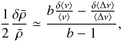 (26)where b is the exponent involved in the power law describing the unknown surface effects, and ⟨ ν ⟩ an average of the frequencies. Interesting limiting cases of the above equation are
-
b = 0: this corresponds to fitting the large frequency separation and brings us back to the previous section;
-
b → ∞: this corresponds to fitting the average frequency, ⟨ ν ⟩ , directly.
One will also note that b = 1 is a singular case which corresponds to a degeneracy in the equations. Kjeldsen et al. (2008) found b = 4.9 for the Sun and consequently used this value for other stars. We will do likewise in what follows.
In practice, we will use Eq. (22) to obtain the large frequency separation, and a similar equation to obtain the average frequency: 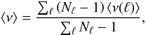 (27)thereby extending this method to non-radial modes. Once more, it is straightforward to see that this approach is unbiased.
4. Non-linear extension
The above procedures are linear and are therefore only adapted to reference models which are sufficiently close to the observed star. However, one may try to extend their applicability by pre-scaling the reference model so as to approach the mean density of the star and hopefully bring the relative differences into the linear regime. We therefore introduce a scale factor s, such that the mean density of the scaled reference model is  and the corresponding frequencies
  . With this rescaled model, the frequency shifts then take on the following expression:
 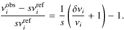 (28)The inverted mean density becomes
 ![Mathematical equation: \begin{equation} \bar{\rho}_{\mathrm{inv}}(s) = \bar{\rho}_{\mathrm{ref}} s^2 \left\{1 + \sum_i c_i \left[ \frac{1}{s}\left(\frac{\delta\nu_i}{\nu_i} + 1\right) - 1\right] \right\}. \label{eq:rho_inv} \end{equation}](/articles/aa/full_html/2012/03/aa18156-11/aa18156-11-eq115.png) (29)If one assumes that the linear inversion procedure is unbiased, then Eq. (29) can be simplified as follows, using Eq. (13):
(29)If one assumes that the linear inversion procedure is unbiased, then Eq. (29) can be simplified as follows, using Eq. (13):  (30)Equation (30) is a second-order equation with the following maximum value:
  (31)where
  (32)It is this maximum value which we will use as the best mean density estimate. Indeed, if one were to start with a given reference model, obtain a first mean density estimate through a given linear inversion, scale the reference model using this mean density, re-apply the inversion to obtain a second mean density, re-scale the reference model, and iterate till convergence, then the final mean density would be
  . Another way of looking at this is that smax is the scale factor for which the inversion yields no further correction to the mean density:
 ![Mathematical equation: \begin{equation} \sum_i c_i \left[ \frac{1}{\smax}\left(\frac{\delta\nu_i}{\nu_i} + 1\right) - 1\right] = 0. \end{equation}](/articles/aa/full_html/2012/03/aa18156-11/aa18156-11-eq121.png) (33)It is then interesting to compare the result from a non-linear procedure to the value obtained from the linearised version of the procedure. If we start with the scaling law between the large frequency separation and the mean density, then the value from the linearised procedure is
(33)It is then interesting to compare the result from a non-linear procedure to the value obtained from the linearised version of the procedure. If we start with the scaling law between the large frequency separation and the mean density, then the value from the linearised procedure is  (34)where we have used Eq. (2). This is identical to what is given directly by the original, non-linearised, scaling law, hence providing additional justification for choosing as the mean density estimate. If we calculate for the linearised version of the KBCD approach, the result is
  (35)This time the result is different from what is given by the original non-linear procedure. However, this difference turns out to be minute. Indeed, Eq. (35) corresponds to the result which would be obtained had the unknown surface effects been represented as a power law in terms of the reference frequencies rather than the observed ones. Using this formulation, the exponent obtained in the solar case becomes 4.86 instead of 4.89, and mean density estimates are hardly affected (for b fixed at 4.9). Hence, in what follows, we will use this formulation as representative of the KBCD approach.
Finally, the associated 1σ error bar on the estimated mean density is now given by  (36)where we have assumed that σi ≪ 1. This is different from what is given in Eq. (12) due to the extra term smax.
By construction, does not depend on the mean density of the initial reference model as opposed to a linear inversion result (this can also be shown explicitly through Eqs. (31) and (32)). The same also applies to  . Furthermore, the various individual kernels, the averaging and cross-term kernels, and the target function remain unchanged since they are non-dimensional and consequently do not depend on the scale factor. As such, they remain a useful diagnostic of the inversion procedure. However, when calculating the error as based on Eq. (10), the relative difference on the density profile needs to take into account the scaling by smax:
 ![Mathematical equation: \begin{equation} \left(\frac{\delta\rho}{\rho}\right)_{\mathrm{scaled}} = \frac{1}{\smax^2} \left[ \left(\frac{\delta\rho}{\rho}\right)_{\mathrm{unscaled}} + 1 \right] - 1. \end{equation}](/articles/aa/full_html/2012/03/aa18156-11/aa18156-11-eq127.png) (37)
(37)
5. The solar case
In order to illustrate the above methods, we applied them to the Sun. A set of 104 GOLF frequencies and associated error bars (Lazrek et al. 1997) were used as observations. We only used the frequencies with a signal-to-noise ratio greater than 1, i.e. those which were not in brackets in Table 1 of Lazrek et al. (1997). The n and ℓ values of these modes are given in Table 1, and the average of the error bars on these frequencies is 0.694 μHz. Model S (Christensen-Dalsgaard et al. 1996) was used as the reference model. It is well known that there are surface effects in the Sun which are not accounted for in Model S. This causes the high-order modes to differ in frequency from the observed values, as is illustrated in Fig. 1. For the sake of comparison, the large frequency separation is also indicated in the figure. The pulsation modes were calculated with ADIPLS (Christensen-Dalsgaard 2008), using an isothermal outer boundary condition, and the inversions were carried out using an improved (and corrected) version of InversionKit1.
The n and ℓ values of the 104 modes from Lazrek et al. (1997).
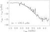 |
Fig. 1 Differences between observed solar cyclic frequencies and those obtained from Model S, using the ℓ = 0 − 5 frequency set from Lazrek et al. (1997). The vertical grey lines indicate the 1σ observational error bars. The large frequency separation is also indicated. |
Before giving the inversion results, it is useful to discuss what the latest and hopefully most accurate value of the solar mean density is. The mass and radius used in Model S correspond to the values given in Allen (1973). Since then, the solar radius underwent a downward revision (Brown & Christensen-Dalsgaard 1998) following a discrepancy with the radius inferred from solar f-modes (Schou et al. 1997; Antia 1998). Further revisions can be found in Haberreiter et al. (2008), who also point out the need for a generally accepted definition. The solar mass is determined by calculating the ratio GM⊙/G, where GM⊙ is known from planetary motions and G, the gravitational constant, from various experiments. The product GM⊙ is known to a high degree of accuracy so the main source of uncertainty comes from the value of G. A summary of the latest values as well as those used in Model S can be found in Table 2. As can be seen in Table 2 (fifth row), the latest mean density represents a 0.14 ± 0.09% increase over the value used in Model S. However, given that the pulsation frequencies scale with , it is not possible to distinguish between a variation on the solar mass and a modification of the gravitational constant from frequency data alone. Hence, it is more appropriate to compare  between Model S and the Sun. As can be seen in the last row, the latest value represents a 0.16 ± 0.08% increase over the value from Model S. This corresponds to what one would expect from inversions if these were exact. Given the excellent agreement between GM⊙ from Model S and the latest value (Table 2, first row), the main contribution to this difference comes from the discrepancy on the radius.
Solar mass and radius.
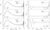 |
Fig. 2 Averaging and cross-term kernels from solar inversions for various parameter settings. No surface corrections are included in the inversion (Msurf = 0). |
Table 3 lists the results for SOLA inversions with various parameter settings, and for a ⟨ Δν ⟩ scaling. The corresponding averaging and cross-term kernels are shown in Fig. 2. The first two columns give the values of β and θ, when relevant. No surface corrections are included in the SOLA approach (i.e., Msurf = 0 in Eq. (16)). The third column gives the relative mean density variation (taking into account the non-linear generalisation described in Sect. 4). Evidently, all inversions predict a slight decrease of the mean density, as opposed to the 0.16% increase expected from the latest solar parameters. This is likely to be caused by poorly modelled surface effects. However, we do note that the ⟨ Δν ⟩ scaling is much more affected, which is not surprising given that the sound travel-time integral is dominated by the near-surface contribution. The next column gives the 1σ error bar around  resulting from the measurement uncertainties on δνi/νi. Finally the last two columns give ∥ Kavg − T ∥ 2 and ∥ Kcross ∥ 2, which intervene in the upper bound on the error, as given in Eq. (11).
Solar inversion results using different schemes for correcting surface effects.
As for most inversion methods, the results are a trade-off between minimising the effects of measurement errors and cross-talk from δΓ1/Γ1 and optimising the averaging kernel. The parameters β = 10-8, θ = 10-4 seem to be a good compromise. If β is increased to 10-1, the inversion wastes much effort trying to reduce the cross-talk from δΓ1/Γ1, which is expected to be small. Although ∥ Kcross ∥ 2 is somewhat reduced, the inversion result is worse and has noticeably increased. If instead θ is reduced to 10-6, the inversion result is slightly better, as is ∥ Kavg − T ∥ 2, but both and ∥ Kcross∥2 take on high values.
5.1. Near-surface effects
It is then interesting to look at different ways of correcting surface effects. Traditionally, these effects have been modelled as an additive term made up of an unknown function of frequency only, Fsurf, normalised by Qi, the mode inertia divided by the inertia of a radial mode interpolated to the same frequency (Christensen-Dalsgaard & Berthomieu 1991). One way of dealing with this term in a SOLA inversion is to treat the function Fsurf as a slowly varying function of ν, such as a linear combination of the first Msurf Legendre polynomials, and then to constrain the inversion to cancel out any such function (Däppen et al. 1991, also see Eq. (16)). The first row of Table 4 gives the inversion result and characteristics for Msurf = 1, which amounts to treating Fsurf as a constant. The corresponding averaging and cross-term kernels are given in the top panels of Fig. 3. Obviously, the results are quite poor. A likely reason for this behaviour is that the function Fsurf is not satisfactorily described by a constant. Instead, judging from Fig. 1, and remembering that Qi is normalised in such a way as to be close to 1 for low ℓ values, |Fsurf| starts at low values and increases with frequency.
One way of trying to deal with this problem is to normalise the function Fsurf in a different way, before treating it as a linear combination of slowly varying functions. Two alternatives are 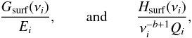 (38)where we have used the notation Gsurf and Hsurf to distinguish these functions from the original function Fsurf, and where Ei is the mode inertia and b the exponent from the KBCD approach. The first possibility is based on the following reasoning. In the original description, the quantity Qi was introduced to replace Ei as it does not vary by several orders of magnitude over the p-mode frequency range (Christensen-Dalsgaard & Berthomieu 1991). However, factoring out this strong variation from Ei also means introducing it into Fsurf. Therefore, normalising by Ei instead of Qi avoids this problem. The second possibility is based on the idea that
  , based on Kjeldsen et al. (2008). Hence by dividing both sides by νb − 1, one is left with a function Hsurf which is slowly varying.
Rows 2–4 of Table 4 give the results from applying these two alternative normalisations, and the corresponding kernels are shown in Fig. 3. In the first two cases, only one (constant) term is used to correct surface effects. The results are slightly better than when no surface corrections are included, with a slight preference for the ν − b + 1Qi normalisation. At the same time, both the averaging kernel and are slightly worse. In the last case, Msurf = 7 in accordance with the optimum number of terms found in Rabello-Soares et al. (1999). However, this leads to poor results. The main difference between the inversions carried out here and those carried out in Rabello-Soares et al. (1999) is the number of modes involved in the inversion. Given the limited number used here (which still remains generous in comparison with stars other than the Sun), one cannot afford to over-correct for surface effects. However, even when no surface corrections are explicitly included, Table 3 shows that a SOLA inversion is less affected by surface effects than a ⟨ Δν ⟩ scaling, probably because as Kavg approaches the target function T, its surface amplitude is reduced.
Another way to try to limit surface effects is to perform a SOLA inversion using only kernels based on frequency separation ratios. Indeed, Roxburgh & Vorontsov (2003) showed that these ratios are insensitive to surface conditions through analytical developments based on internal phase shifts and through numerical simulations. Likewise, Otí Floranes et al. (2005) showed that the associated kernels have a small amplitude near the surface. However, they also pointed out that both the numerator and denominator of a frequency separation ratio scale with , meaning that the ratio is insensitive to the mean density of the underlying model. As a result, the ci coefficients associated with an inversion based on these kernels add up to 0, making it impossible to perform an unbiased inversion. Likewise, it can be shown using Eq. (14) that the integral of the kernels  is approximately 0.
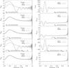 |
Fig. 3 Averaging and cross-term kernels from solar inversions for different treatments of surface effects. The last row shows the averaging and cross-term kernels from the KBCD approach rather than from a SOLA inversion. |
Finally, the last row of Table 4 gives the results from applying the KBCD approach. The associated averaging and cross-term kernels are displayed in the lower panels of Fig. 3. The mean density estimate and compare favourably with the other inversion results and the associated kernels are well-behaved, thus explaining why this method works. This approach is found to be superior to the simple scaling law based on the large frequency separation, as can be seen both in terms of the results it produces and in terms of the kernels. The likely reason for this is that the averaged frequency, which intervenes in this approach, uses a more uniform weighting on the individual frequencies, whereas the large frequency separation favours frequencies at either end of the frequency range, thus amplifying surface effects, which are strongest at high radial orders. Overall, the best results are obtained with the ν − b + 1Qi normalisation, using one term for surface effects, and the KBCD approach (third and fifth line of Table 4).
6. Test cases with a grid of models
In order to conduct a more systematic study, we applied the different inversion procedures to a grid of 93 main-sequence and pre-main-sequence models. These models were downloaded from grid B of the CoRoT-ESTA-HELAS website2, and were chosen within the (Teff,log (g)) box (5291 ± 100 K,4.563 ± 0.1 dex), the error bars being representative of what can be expected from spectroscopic observations. Their masses range from 0.80 M⊙ to 0.92 M⊙ and their ages from 28 Myr to 17.6 Gyr after their appearance on the birthline. A description of the physical ingredients, chemical composition and initial conditions used in these models is given in Marques et al. (2008). In particular, the initial chemical composition is (X,Y,Z) = (0.70,0.28,0.02), where the metal abundances correspond to the solar mixture given in Grevesse & Noels (1993). Figure 4 shows the positions of these models in a (Teff,log (g)) diagram, along with some evolutionary tracks, the dashed parts corresponding to the pre-main-sequence. Three additional models, nicknamed “Models A, A′ and B”, were selected near the centre of this box to play the role of observed stars. These models are also shown in Fig. 4, and Table 5 gives some of the characteristics of Models A and B. The frequencies of these models are shown in an échelle diagram in Fig. 5. In all cases tested here, the 1σ error bar on the frequencies was set at 0.3 μHz, although no errors were added to the frequencies. The goal of this study is then to see how well the density of these three models can be reproduced by applying the various inversion procedures to the models from the grid.
 |
Fig. 4 Teff − log (g) diagram showing the position of Model A (◇), Model B (□), the reference models from grid B ( + ), and various pre-main-sequence and main-sequence tracks, represented by the dashed and continuous line, respectively. |
6.1. Model A
Model A represents a 0.9 M⊙ main-sequence star and was downloaded from grid A of the CoRoT-ESTA-HELAS website3 Models from grid A are started off as fully convective spheres, instead of using a birthline as in grid B. Apart from this difference, this model has the same chemical composition and physical ingredients as the models in the grid.
Each one of the models from the grid was used as a reference model from which to apply the different inversion techniques to the “observed” frequencies from Model A. Figure 6 shows the results from these inversions for a set of 33 modes with radial orders n = 15−25 and harmonic degrees ℓ = 0−2. The parameter β was set to 10-8 for all SOLA inversions. Although the mean densities of the reference models differ from that of Model A by up to 30% (see the x-axis in figures), the inversion results are within 0.3 to 0.6% of the true mean density except for the worst cases where the departure can exceed 1.0%, which shows the sensitivity of these modes to density. A more detailed look at the figures shows that overall, the KBCD approach and SOLA inversions produce the best results, provided the parameter θ is not too small. The two are very similar if Msurf = 1, θ = 10-2 and a ν − b + 1Qnℓ normalisation is used for surface effects. The large frequency separation, for the most part, produces results which are worse. One may also notice that in most cases, the difference between the inverted and true mean densities is much larger than the 1σ error bar from the inversions. This behaviour can be expected, since the 1σ error bar from the inversion is only based on the frequency measurement errors and does not take into account the other sources of error mentioned in Sect. 2.3, such as differences between the averaging kernel and the target function or cross-talk from the δΓ1/Γ1 profile.
Characteristics of Models A and B.
Evidently, reducing θ mainly seems to increase the 1σ error bar in SOLA inversions without improving the results. This can be understood by looking at the trade-off curves illustrated in Fig. 7. Indeed, reducing θ only has a small effect on ∥Kavg − T∥ 2 while increases substantially. Furthermore, the same mechanism which amplifies observational errors can also amplify errors which are not accounted for in Eq. (10), such as non-linear effects not included in Eq. (1) or numerical errors on kernel calculations. Based on Figs. 6 and 7, the value θ = 10-2 seems to be a good compromise between the two effects.
Furthermore, given that the true structure of Model A is known, it is possible to analyse the different sources of error based on Eq. (10). These are displayed in Fig. 8 for SOLA inversions. The dominant contribution comes from a mismatch between the averaging kernel and the target function and is represented by a solid line. The dotted line represents the cross-talk from the δΓ1/Γ1 profile and is the smallest contribution. Lastly, the dashed curve represents remaining effects such as surface contributions, measurement errors on the frequencies and effects not included in Eq. (10), such as non-linear effects not accounted for in Eq. (1). Of these three, the non-linear effects are likely to be the strongest because the data is error-free (except for numerical round-off errors) and no attempt was made to simulate surface effects in Model A. Obviously, the non-linear effects are not negligible compared to the other sources of error. This is not entirely surprising given that the only criteria used for selecting the models from the grid was the (Teff,log (g)) error box, and consequently shows the limits of Eq. (1). It must also be noted that the errors in Fig. 8 tend to compensate for each other. However, one cannot always expect such a fortuitous cancellation to arise in other situations.
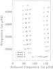 |
Fig. 5 Echelle diagram with the frequencies from Models A, A′ and B. The ℓ = 2 and ℓ = 0 ridges are to the left, while the ℓ = 1 ridge is to the right. Note: the large frequency separation indicated in the lower right corner is the value used to construct this figure, not necessarily the exact value for the three models. |
Figure 9 shows what happens if the non-linear extension described in Sect. 4 is not applied to the inversion procedures. As expected, inversion results are substantially worse when the mean density of the reference models is far from the true mean density.
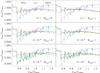 |
Fig. 6 Inversion results for Model A, using the modes with n = 15−25 and ℓ = 0−2. The x axis gives the mean density of the reference models divided by that of Model A, while the y axis is the mean densities obtained from the various inversion procedures, normalised by that of Model A. For each procedure, there are three lines corresponding to the result and the 1σ error bar around it. The horizontal triple-dot-dashed line shows the correct mean density. A ν−b + 1Qnℓ normalisation has been used when surface corrections are included in SOLA inversions. |
Finally, the wiggles observed in Fig. 6, especially for reference models with a lower mean densities, can be partially explained by the fact that the grid contains a mixture of pre-main-sequence and main-sequence models. Indeed, when the two types of models are separated as in Fig. 10, two separate trends can be observed which likely reflect their differences in structure.
6.2. Near-surface effects (Model A′)
Model A′ is nearly identical to Model A, except for an ad hoc 50% increase of the density in the outer 1% of the model, the transition being represented by a hyperbolic tangent function. The pressure was then recalculated using the hydrostatic equation, thus resulting in a very slight offset from the original profile. The difference in mean density between the two models is negligible, but the frequencies are noticeably different (see Fig. 5) because sound waves spend more time in the outer layers of a star.
Figure 11 shows the inversion results for this model, using the same set of modes as in the previous case. Overall, the results are worse than in the previous case. Furthermore, the scaling law based on the large frequency separation yields results which are substantially offset from the true mean density, when compared to the other procedures. This could be expected because the large frequency separation, which asymptotically gives the travel time of a sound wave from centre to surface, is very sensitive to surface conditions. This high sensitivity to surface conditions is also reflected in the associated averaging kernels which tend to have large amplitudes near the surface. The SOLA inversions without surface corrections also seem to be affected, but to a lesser degree. In particular, it produces worse results than the KBCD approach for the higher density models, which is the opposite from the previous case. If surface corrections are included in the SOLA approach, they produce slightly better results than the KBCD approach. Once more, reducing θ does not improve the SOLA inversions, but only serves to increase the 1σ error bar.
6.3. Uncertainties in the stellar physics (Model B)
Model B is different in a number of ways from Model A and also from the models in the grid. It has a different chemical composition and includes the effects of diffusion and rotational mixing, thereby providing a way to test the effects of unknown physics on mean density inversions. Specifically, the chemical abundances are (X,Y,Z) = (0.735,0.250,0.015) and follow the more recent solar mixture given in Asplund et al. (2005).
The results are shown in Fig. 12, using once more the same set of modes. These results are indeed similar to those obtained for Model A and show that all inversion procedures presented here seem to be fairly robust to unknown physics.
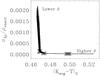 |
Fig. 7 Superimposed trade-off curves for each of the 93 models from the grid. The parameters are Msurf = 0, β = 10-8 and θ = 10-6, 10-4, 10-2, 1, 1.5. The grey “ × ” marks the locations of intermediate θ values. |
 |
Fig. 8 Different sources of error based on Eq. (10) for SOLA inversions. See text for details (in particular for “Other”). The SOLA parameters are β = 10-8, θ = 10-2 and Msurf = 0. |
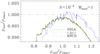 |
Fig. 9 Same as Fig. 6(right, middle panel), except that the non-linear extension described in Sect. 4 has not been applied to the inversion procedures. |
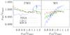 |
Fig. 10 Same as Fig. 6(left, middle panel), except that the pre-main-sequence models (left panel) and the main-sequence models (right panel) have been separated. |
6.4. The effects of mode misidentification
We then investigated the effects of misidentifying the radial orders of the modes. Figure 13 (left panels) shows mean density estimates for Model A, using the same set of observed modes as previously, but identified as n = 16−26 (upper panel) and n = 14−24 (lower panel). As can be seen in these figures, the scaling law based on the large frequency separation provides the best results, whereas the other methods are off by 10%. A simple explanation is that the relative change over one radial order of Δν is smaller than that of ν, given that Δν goes to a constant when n goes to infinity, whereas ν is roughly proportional to n.
Another way of misidentifying modes is by labelling the ℓ = 0 modes as ℓ = 1 and vice-versa (e.g. Benomar et al. 2009a). This, however, also leads to detecting a different set of ℓ = 2 frequencies because these will always be close to the ℓ = 0 frequencies. In order to investigate this scenario, we swapped the ℓ = 0 and 1 identifications and created a fictitious set of ℓ = 2 frequencies in such a way as to preserve the original small frequency separation, averaged over adjacent radial orders. Two possible ways of assigning radial orders exist and are given in Table 6. The corresponding mean density estimates are given in the right-hand panels of Fig. 13. Once more, the large frequency separation gives the best results, the other methods being off by about 5%, i.e. by about half the amount compared to the previous case when only n was misidentified. One way of interpreting this is to view this as a ± 1/2 offset on the radial order, and then to apply the same argument as above.
These observations provide a way of identifying modes: one can calculate the mean density using the large frequency separation and another method such as the KBCD approach or a SOLA inversion and search for the values of ℓ and n, for which the two methods agree to within 1% or so. This procedure, although different from the methods described in Bedding & Kjeldsen (2010) and White et al. (2011), is based on the same principles. Indeed, the method presented here and the approach from Bedding & Kjeldsen (2010) both amount to scaling a model (or a comparison star) so that the large frequency separation agrees with that of the observed star, then adjusting the identification so that the offset between the two sets of frequencies is minimised. White et al. (2011) achieve the same result by directly comparing their model-based values for the large frequency separation and ϵ, the additive offset from the asymptotic formula for p-mode frequencies, to those from observed stars. Of course, surface effects acting upon the large frequency separation may lead to an offset even for the correct identification, although we expect such an offset to be smaller than what is shown in Fig. 11, which was calculated for a fairly drastic modification of the surface. White et al. (2011) have nonetheless pointed out situations where ϵ can vary rapidly, which makes mode identification more difficult.
6.5. Kernel mismatch
It it also interesting to test the various inversion techniques on different sets of modes. We therefore considered the following 2 sets:
-
Set 1: n = 2−10 for ℓ = 0,2,3, n = 5−10 for ℓ = 1, n = 1−10 for ℓ = 4.
-
Set 2: the same as Set 1 without the n = 1, ℓ = 4 mode.
The mean density estimates are shown in Fig. 14. As can be seen by comparing the two figures, including the n = 1, ℓ = 4 mode has a drastic effect on the SOLA inversion result for one of the models, which we shall call the “worst model”. The explanation for this is quite simple. Figure 15 shows the kernels associated with this mode for the worst model and for Model A. Clearly, the kernels in the worst model are dominated by a g-mode behaviour (even if the eigenfunctions still seem to be dominated by a p-mode character), whereas those of Model A are typical of p-modes. This difference on the kernels inevitably leads to a large discrepancy between the actual frequency shift for that particular mode and the frequency shift which would be deduced by applying the linear approximation given in Eq. (1). This, of course, affects any mean density estimates, particularly a SOLA inversion which explicitly optimises the averaging and cross-term kernels using the individual kernels.
7. Observed stars
7.1. α Cen B
Having tested the inversion techniques on stellar models in a number of ways, we now try them out on observed stars. A particularly interesting example is the nearby K1 main-sequence star α Cen B. Its close proximity allows precise interferometric measurements of its angular radius (Kervella et al. 2003). When combined with a reprocessed Hipparchos parallax (Söderhjelm 1999), this yields a radius R = 0.863 ± 0.005 R⊙. Given that α Cen B is part of a multiple system, it is possible to determine its mass through orbital parameters. Hence, Pourbaix et al. (2002) obtained a mass of M = 0.934 ± 0.0061 M⊙ using the parallax from Söderhjelm (1999). This then yields a mean density of 2.046 ± 0.058 g cm-3. A time series of radial velocities was obtained by Kjeldsen et al. (2005) using the Very Large Telescope (VLT) and the Anglo-Australian Telescope (AAT). A Fourier analysis of this time series yielded a set of 37 frequencies with harmonic degrees ℓ = 0 to 3, and radial orders, n, between 17 and 32.
Given that the mass of α Cen B is close to the mass range covered by the grid from the previous section, we simply reused the models from this grid as reference models from which to estimate the mean density of α Cen B. The results are shown in Fig. 16. These turn out to be similar to the results obtained in the previous sections. The tendencies are the same, as is the spread in inverted mean densities, except for the results from the ⟨ Δν ⟩ scaling where the spread is somewhat larger. Nonetheless, a noticeable difference appears between the estimates from the ⟨ Δν ⟩ scaling and the two other methods. This suggests that surface effects play an important role in this star.
It is then interesting to see how these densities compare with previous studies. Table 7 gives a summary of previous and current estimates of the mean density of α Cen B. As was mentioned above, the mass from Pourbaix et al. (2002) and the radius from Kervella et al. (2003) lead to a mean density of 2.046 ± 0.058 g cm-3. The results from the KBCD and SOLA approaches are 2 to 3% lower than this value, but remain within the error bars. They agree with the range of values, delimited by the triple-dot-dashed horizontal lines in Fig. 16, obtained in Kjeldsen et al. (2008) where the KBCD approach is developed. The seismic study in Eggenberger et al. (2004) leads to a mean density of 1.998 g cm-3, which also falls within this range, although they did increase the error bar on the radius to reach this value (the error bar on the mass seems to have been ignored in their study). On the other hand, the ⟨ Δν ⟩ scaling leads to values below all of these previous studies and which mostly lie outside the error bars of the non-seismic mean density. Hence, using the KBCD or SOLA approaches leads to better agreement with the non-seismic constraints and tends to confirm the idea that the ⟨ Δν ⟩ scaling is affected by surface effects.
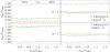 |
Fig. 13 Inversion results for Model A, using the same modes as in Fig. 6 but with various erroneous mode identifications, as indicated in the panels. In all panels, β = 10-8, θ = 10-4 and Msurf = 0. |
Different ways of assigning radial orders when misidentifying the ℓ value.
7.2. HD 49933
We now turn our attention to stars observed by CoRoT. A particularly interesting example is the F5 main-sequence star HD 49933, which has been observed in two separate CoRoT runs, thereby yielding a rich frequency spectrum. In what follows, we will use the set of 51 frequencies and associated error bars and identifications given in Benomar et al. (2009b), which takes into account the two observational runs. An alternative identification had been favoured before data from the second observational run were available (e.g., Appourchaux et al. 2008). The grid of models used in the previous sections is not suitable for this star. We therefore downloaded a set of 42 pre-main-sequence and main-sequence models from the CoRoT-ESTA-HELAS website, which lie in the error box Teff = 6665 ± 215 K and log (L/L⊙) = 0.54 ± 0.02 dex, based on the values quoted in Benomar et al. (2010) and references therein. No attention was paid to possible differences in chemical composition between these models and HD 49933.
The mean density estimates are given in Fig. 17. They fall in the interval 0.580 ± 0.015 g cm-3, which corresponds to a ± 2.6% range around the mid-value. This interval is on the lower end of the range of values covered by the reference (or input) mean densities. Furthermore, the estimated mean density slightly increases with the reference mean density, in much the same way as in the previous examples but on a larger scale. If we limit ourselves to reference models with a closer mean density to the results, this would favour the lower values, but this reasoning must be taken with some caution since the inversions use the non-linear extension and are therefore insensitive to the mean density of the input models. Various other groups have performed detailed asteroseismic interpretations of his star and have come up with best-fitting models using a variety of techniques. Here, we will only focus on studies for which both the mass and radius of the best-fitting model are provided. Kallinger et al. (2010) searched for a best-fitting model in a dense grid using a χ2 criteria, whereas Creevey & Bazot (2011) found two solutions using both a Levenberg-Marquardt and a Markov Chain Monte Carlo approach. Their results are summarised in Table 8 and represented as triple-dot-dashed horizontal lines in Fig. 17. The first solution uses a mode identification in which the ℓ values are swapped. Its mean density lies in the upper half of the range of values found here. The two other solutions use the same identification as the one used here. They have very similar mean densities in spite of having different radii and masses, and are at the lower end of the interval of solutions found here. Although deviating more from our mid-value, these solutions are located where the mean densities are least modified by the inversions.
Given the difficulties in labelling the modes prior to the second CoRoT run, we tested the swapped ℓ identification, using only the ℓ = 0 and 1 modes. The results are shown in Fig. 18 and are very similar to the results presented in Fig. 13. Clearly, the models used in this study favour the currently accepted identification. In particular, this agrees with the identification favoured by Kallinger et al. (2010) and with the results from Bedding & Kjeldsen (2010), who compared HD 49933 to other observed stars whose identification is known.
Finally, it is worth noting that surface effects have not manifested themselves in the results presented here: all three methods yield similar results for the correct identification. This suggests that surface effects are less important in this star compared to other effects deeper within the star. Interestingly, Bedding et al. (2010) recently reported on an asteroseismic investigation of Procyon, also of spectral type F5. They showed that the KBCD approach with a solar exponent, b = 4.9, did not provide a good description of the differences between the frequencies of various best-fitting models and those of the star. Instead, these were better described as a constant offset, which corresponds to b = 0. Because these differences do not go to zero when the frequency is reduced, the authors also interpreted this as signifying that the structural differences between their best-fitting models and Procyon extend beyond the surface layers.
7.3. HD 49385
The star HD 49385 is an evolved G0 type star which was observed by CoRoT for 137 days during its second long run. Deheuvels et al. (2010) were able to detect 27 ℓ = 0−2 frequencies as well as what seems to be mixed modes and some unconfirmed ℓ = 3 frequencies. In what follows, we will not use the ℓ = 3 modes because of their low signal-to-noise ratio, and will postpone dealing with the mixed modes to the end of this section, because they vary rapidly from one model to another, thereby limiting the validity of Eq. (1). A new set of 18 models within the (Teff,log (g)) = (6095 ± 65 K, 4.00 ± 0.06) error box (Deheuvels et al. 2010) was downloaded from the CoRoT-ESTA-HELAS website. Given the position of this box in the HR diagram, these models correspond to either pre- or post-main-sequence stars4.
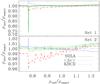 |
Fig. 14 Inversion results for Model A for two similar sets of modes (see text for details). The parameters used in these inversions are β = 10-8, θ = 10-4 and Msurf = 0. |
The mean density estimates are given in Fig. 19. The horizontal triple-dot-dashed lines are the mean densities corresponding to the four families of solutions in Deheuvels & Michel (2011). In the upper panel, the results are particularly poor. This failure is caused by differences in mode labelling between the pre- and post-main-sequence models owing to the presence of mixed modes in the latter. The inversion results were based on an identification which corresponds to some of the best-fitting models from Deheuvels & Michel (2011), who applied Newton’s method to a grid of models specifically designed to handle mixed modes. Such an identification is ill-adapted for pre-main-sequence models and to a lesser extent for some of the post-main-sequence models because of the jumps it introduces in the n values. Consequently, the results from the five pre-main-sequence models, indicated by the circles, stand out as being the worst. In order to circumvent these difficulties, a second inversion was carried out, only using the ℓ = 0 modes. This time, the results are far better and are within 2.5% of the mean densities from Deheuvels & Michel (2011) for the SOLA inversions and for the KBCD approach, and 3.5% for the scaling law based on the large frequency separation. Paradoxically, the pre-main-sequence models now give the results which are closest to Deheuvels & Michel (2011). Once more, the scaling law is somewhat different from the two other approaches, which is probably indicative of surface effects.
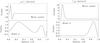 |
Fig. 15 Kernels of the n = 1, ℓ = 4 mode for Model A (lower panels) and the worst model (upper panels). |
In order to investigate the influence of mixed modes on SOLA mean density inversions, we used a low-overshoot model from Deheuvels & Michel (2011) with the Asplund et al. (2005) mixture. Inversions were carried out for three different sets of modes:
-
Set 1: 26 p-modes with ℓ = 0 − 2.
-
Set 2: Set 1 + the (n = 14,ℓ = 1) p-mode.
-
Set 3: Set 1 + the (n = 10,ℓ = 1) mixed mode5.
Two different sets of SOLA parameters were used:
-
Case 1:β = 10-8, θ = 10-2 and Msurf = 1. These parameters were chosen in accordance with typical inversion parameters (the number of modes was sufficient to allow Msurf = 1).
-
Case 2: β = 0, θ = 0, Msurf = 0. These parameters correspond to optimising Kavg only.
The results are summarised in Table 9. As can be seen in case 1, adding a p-mode or a mixed mode has a similar impact on both the averaging kernel and the cross-term kernel. The reduction of the statistical error on the inverted mean density,  , is higher for the mixed mode than for the p-mode, indicating that the mixed mode may be yielding more information on the mean density. This seems to be confirmed in case 2, where only the averaging kernel is being optimised. Indeed, the averaging kernel including the mixed mode is closer to the target function than the averaging kernel which uses the extra p-mode. However, the extra benefit from the mixed mode remains small and is probably of little use because the domain for which Eq. (1) is valid is likely to be much smaller for these modes than for ordinary p-modes. In some cases, non-linear effects on these modes can even cause a substantial error on the mean density, as was shown in Sect. 6.5.
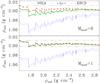 |
Fig. 16 Mean density estimates for α Cen B. The SOLA parameters are β = 10-8 and θ = 10-2, and Msurf is indicated in the panels. The vertical triple-dot-dashed line corresponds to the minimum and maximum mean densities from Kjeldsen et al. (2008). |
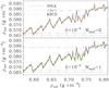 |
Fig. 17 Mean density estimates for HD 49933. The SOLA parameters are β = 10-8 and θ = 10-2. The horizontal triple-dot-dashed lines represent the solutions from Creevey & Bazot (2011) and Kallinger et al. (2010), in the same order as in Table 8. |
Does this mean that mixed modes are therefore not a useful diagnostic of core conditions, and that previous studies somehow exaggerated their importance? Certainly not. Rather, it means that the methods presented here are not as efficient at exploiting the full diagnostic potential of these modes. Other methods, such as that presented in Deheuvels & Michel (2011), or inversions localised around the stellar core, are needed to fully benefit from these modes. A possible explanation for this failure can be described as follows. Structural kernels associated with mixed modes and g-modes, such as those illustrated in the upper panels of Fig. 15, show a strong oscillatory behaviour near the centre of the star, which does not match the target function, T, defined Eq. (17). As a result, their contribution to SOLA inversions tends to be reduced, as reflected, to some extent, in their inversion coefficients. On the other hand, their contribution is not reduced in the KBCD approach or the ⟨ Δν ⟩ scaling law, and this consequently leads to averaging kernels with highly oscillatory behaviour near the centre, which can also be a source of error.
8. Discussion and conclusion
We have investigated different techniques for estimating directly the mean density of a star. These include the usual scaling law based on the large frequency separation, an approach described in Kjeldsen et al. (2008) (the “KBCD approach”), and a SOLA inversion technique with a non-linear extension. We have shown how all three techniques can be put in a similar form, which allows the construction of associated averaging and cross-term kernels, useful for characterising what is actually being measured and for quantifying the error.
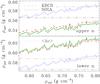 |
Fig. 18 Mean density estimates for HD 49933 using swapped ℓ identifications. The SOLA parameters are β = 10-8, θ = 10-2 and Msurf = 1. The solutions from Creevey & Bazot (2011) and Kallinger et al. (2010) are represented as triple-dot-dashed horizontal lines. |
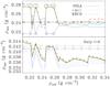 |
Fig. 19 Mean density estimates for HD 49385. The SOLA parameters are β = 10-8, θ = 10-2 and Msurf = 0. The horizontal triple-dot-dashed lines correspond to the best-fitting models from Deheuvels & Michel (2011). The circled results (upper panel) were obtained for pre-main-sequence models (for clarity, these are not circled in the lower panel). |
A comparison of the three techniques, applied to the Sun and to various test cases, shows that the KBCD approach and SOLA inversions yield similar results, whereas the scaling law based on the large frequency separation produces sub-optimal results. The averaging kernels produced by the KBCD approach can come close in quality to those produced by a SOLA inversion and are substantially better than the averaging kernels associated with the simple scaling law based on ⟨Δν⟩, thereby explaining its relative success. Hence, if one only aims to estimate a mean density and does not need a full diagnostic on the accuracy of the result, the KBCD approach should be sufficient. However, for a more detailed analysis, the SOLA method seems ideal because it is specifically designed to optimise the averaging kernel while reducing various sources of error. Furthermore, possible improvements to the SOLA method, such as introducing weight functions in the cost function Eq. (16) (e.g. Rabello-Soares et al. 1999), may help to fine-tune this method and should therefore be explored.
As expected from asymptotic theory, near-surface effects are shown to have a stronger impact on the ⟨Δν⟩ scaling law than on the two other methods, even when surface corrections are not included in the SOLA approach. However, these two methods require a correct identification of the modes, whereas the ⟨ Δν ⟩ scaling law is much more tolerant of mode misidentification. Hence, looking for an ℓ and n assignment which provides the best agreement between the simple scaling law and one of the two other methods can be a useful way of identifying modes. This approach to mode identification, although different from the methods presented in Bedding & Kjeldsen (2010) and White et al. (2011), is also based on the same principles.
Quantitatively, a precision around 0.5% or better was reached for the Sun, for α Cen B (as based on the spread of the results), and for various test cases using SOLA inversions (with β = 10-8 and θ = 10-2) and the KBCD approach, whereas the scaling law was less accurate with a precision of 1% or worse. However, when applied to two stars observed by CoRoT, the spread in values was larger, up to ±2.5% for the first two methods, and ± 3.5% for the ⟨Δν⟩ scaling law. The reason for this remains an open question, but does not seem to stem from the fact that these are observed stars, as indicated by additional tests involving models instead (results not included) and the results obtained for α Cen B. Rather, it may be that in the part of the HR diagram which contains these stars, there are larger variations in the density profile with stellar evolution. A ± 3.5% spread is comparable to the spread obtained in White et al. (2011) for stars with Teff below 6700 K. Above this temperature, White et al. (2011) obtained larger differences, which in some cases reached 10%, between the true density and that obtained from the ⟨Δν⟩ scaling law. This raises the question as to how accurate the KBCD and SOLA approaches would be in a similar situation, although one also has to bear in mind that this temperature range is less relevant for solar-like oscillations. One notable difference between the results described here and those presented in White et al. (2011) is that the latter are calibrated to solar values rather than nearby reference models, which is likely to be an additional source of error, especially for stars with a large temperature difference with respect to the Sun.
If combined with a 2% error bar on measured radii, as is expected from Gaia, a 2.5% to 3.5% uncertainty on the mean density yields an 8.5−9.5% error bar on the mass of the star, where the dominant contribution to the error comes from the uncertainty on the radius. Such an error bar will then directly translate itself into a comparable uncertainty on the inferred mass of any potential exoplanet (e.g. Guillot & Havel 2011, and references therein). Accordingly, one may try to obtain more accurate results through more complicated approaches such as searching for best-fitting models in a grid or applying non-linear inversion techniques. These approaches will overcome the non-linear effects shown in Fig. 8 and which are beyond the control of the methods presented here. However, given the difficulties in optimising the averaging kernel beyond a certain point for a given set of modes, one is still left with the question as to how much information is intrinsically available in the pulsation frequencies and how much is being assumed in these more sophisticated methods.
Finally, it was shown that the methods presented here do not fully exploit the diagnostic potential of mixed modes. Indeed, mixed modes have kernels with a highly oscillatory behaviour near the centre, which strongly differs from the target function, T, defined in Eq. (17). This reduces the contribution of mixed modes to SOLA inversions and leads to averaging kernels with an oscillatory behaviour near the centre for the ⟨ Δν ⟩ scaling law and the KBCD approach. Also, the linear domain for these modes is smaller and can lead to substantial errors when outside this domain, as shown in Sect. 6.5. However, one may expect these modes to be very useful when applying localised inversion methods to models which are close to the true stellar structure.
This software can be downloaded form the Global Helioseismology HELAS website: http://helas.group.shef.ac.uk/science/inversions/InversionKit/index.php
The specific URL to Model A is http://www.astro.up.pt/corot/models/cesam/A/data/0.90/ms/star_1492.002-ad.osc.gz
As was argued in Deheuvels & Michel (2011), the presence of mixed modes shows that this is a post-main-sequence star. Hence, one would want to limit the inversions to this type of star. However, for the sake of comparison, we will also use pre-main-sequence stars and see what impact this has on the inversions.
We note that there is an offset of 1 between the radial orders used here and the ones used in Deheuvels & Michel (2011). This is merely a difference in mode labelling and consequently does not affect inversion results.
Acknowledgments
We thank the referee for helpful comments and suggestions which have improved the manuscript. We also thank I. Roxburgh, S. Vorontsov and S. Basu for interesting discussions and answers to questions. D.R.R. is supported by the CNES (“Centre National d’Études Spatiales”) through a postdoctoral fellowship. This article made use of InversionKit, an inversion software developed in the context of the European Helio- and Asteroseismology Network (HELAS), which is funded by the European Commission’s Sixth Framework Programme. NCAR is sponsored by the National Science Foundation. D.R.R. also acknowledges financial support through a postdoctoral fellowship from the “Subside fédéral pour la recherche 2011”, University of Liège.
References
- Aerts, C., Christensen-Dalsgaard, J., & Kurtz, D. W. 2010, Asteroseismology (Heidelberg: Springer-Verlag GmbH), 193 [Google Scholar]
- Allen, C. W. 1973, Astrophysical quantities, 3rd edn., ed. C. W. Allen (University of London, London: The Athlone Press) [Google Scholar]
- Antia, H. M. 1996, A&A, 307, 609 [NASA ADS] [Google Scholar]
- Antia, H. M. 1998, A&A, 330, 336 [NASA ADS] [Google Scholar]
- Antia, H. M., & Basu, S. 1994, A&AS, 107, 421 [NASA ADS] [Google Scholar]
- Appourchaux, T., Michel, E., Auvergne, M., et al. 2008, A&A, 488, 705 [NASA ADS] [CrossRef] [EDP Sciences] [Google Scholar]
- Asplund, M., Grevesse, N., & Sauval, A. J. 2005, in Cosmic Abundances as Records of Stellar Evolution and Nucleosynthesis, ed. T. G. Barnes III, & F. N. Bash (San Francisco: ASP), ASP Conf. Ser., 336, 25 [Google Scholar]
- Bazot, M., Bourguignon, S., & Christensen-Dalsgaard, J. 2008, Mem. Soc. Astron. Ital., 79, 660 [Google Scholar]
- Bedding, T. R., & Kjeldsen, H. 2010, Comm. Asteroseismol., 161, 3 [Google Scholar]
- Bedding, T. R., Kjeldsen, H., Campante, T. L., et al. 2010, ApJ, 713, 935 [NASA ADS] [CrossRef] [Google Scholar]
- Benomar, O., Appourchaux, T., & Baudin, F. 2009a, A&A, 506, 15 [NASA ADS] [CrossRef] [EDP Sciences] [Google Scholar]
- Benomar, O., Baudin, F., Campante, T. L., et al. 2009b, A&A, 507, L13 [NASA ADS] [CrossRef] [EDP Sciences] [Google Scholar]
- Benomar, O., Baudin, F., Marques, J. P., et al. 2010, Astron. Nachr., 331, 956 [NASA ADS] [CrossRef] [Google Scholar]
- Brown, T. M., & Christensen-Dalsgaard, J. 1998, ApJ, 500, L195 [NASA ADS] [CrossRef] [Google Scholar]
- Christensen-Dalsgaard, J. 2008, Ap&SS, 316, 113 [NASA ADS] [CrossRef] [Google Scholar]
- Christensen-Dalsgaard, J., & Berthomieu, G. 1991, Theory of solar oscillations, ed. A. N. Cox, W. C. Livingston, & M. S. Matthews (Tucson: University of Arizona Press), 401 [Google Scholar]
- Christensen-Dalsgaard, J., Schou, J., & Thompson, M. J. 1990, MNRAS, 242, 353 [NASA ADS] [Google Scholar]
- Christensen-Dalsgaard, J., Dappen, W., Ajukov, S. V., et al. 1996, Science, 272, 1286 [CrossRef] [Google Scholar]
- Cox, A. N. 2000, Allen’s astrophysical quantities, ed. A. N. Cox (New York: AIP Press, Springer-Verlag) [Google Scholar]
- Creevey, O. L., & Bazot, M. 2011, J. Phys. Conf. Ser., 271, 012038 [NASA ADS] [CrossRef] [Google Scholar]
- Däppen, W., Gough, D. O., Kosovichev, A. G., & Thompson, M. J. 1991, in Challenges to Theories of the Structure of Moderate-Mass Stars, ed. D. Gough, & J. Toomre (Berlin: Springer Verlag), Lecture Notes in Physics, 388, 111 [Google Scholar]
- Deheuvels, S., & Michel, E. 2011, A&A, 535, A91 [NASA ADS] [CrossRef] [EDP Sciences] [Google Scholar]
- Deheuvels, S., Bruntt, H., Michel, E., et al. 2010, A&A, 515, A87 [NASA ADS] [CrossRef] [EDP Sciences] [Google Scholar]
- Eggenberger, P., Charbonnel, C., Talon, S., et al. 2004, A&A, 417, 235 [NASA ADS] [CrossRef] [EDP Sciences] [Google Scholar]
- Gough, D. O., & Thompson, M. J. 1991, The inversion problem, ed. A. N. Cox, W. C. Livingston, & M. S. Matthews (Tucson: University of Arizona Press), 519 [Google Scholar]
- Grevesse, N., & Noels, A. 1993, in Origin and Evolution of the Elements, ed. N. Prantzos, E. Vangioni-Flam, & M. Casse (Cambridge: Cambridge University Press), 15 [Google Scholar]
- Guillot, T., & Havel, M. 2011, A&A, 527, A20 [NASA ADS] [CrossRef] [EDP Sciences] [Google Scholar]
- Haberreiter, M., Schmutz, W., & Kosovichev, A. G. 2008, ApJ, 675, L53 [NASA ADS] [CrossRef] [Google Scholar]
- Kallinger, T., Gruberbauer, M., Guenther, D. B., Fossati, L., & Weiss, W. W. 2010, A&A, 510, A106 [NASA ADS] [CrossRef] [EDP Sciences] [Google Scholar]
- Kervella, P., Thévenin, F., Ségransan, D., et al. 2003, A&A, 404, 1087 [NASA ADS] [CrossRef] [EDP Sciences] [Google Scholar]
- Kjeldsen, H., & Bedding, T. R. 1995, A&A, 293, 87 [NASA ADS] [Google Scholar]
- Kjeldsen, H., Bedding, T. R., Butler, R. P., et al. 2005, ApJ, 635, 1281 [NASA ADS] [CrossRef] [Google Scholar]
- Kjeldsen, H., Bedding, T. R., & Christensen-Dalsgaard, J. 2008, ApJ, 683, L175 [NASA ADS] [CrossRef] [Google Scholar]
- Kjeldsen, H., Christensen-Dalsgaard, J., Handberg, R., et al. 2010, Astron. Nachr., 331, 966 [NASA ADS] [CrossRef] [Google Scholar]
- Lazrek, M., Baudin, F., Bertello, L., et al. 1997, Sol. Phys., 175, 227 [NASA ADS] [CrossRef] [Google Scholar]
- Marques, J. P., Monteiro, M. J. P. F. G., & Fernandes, J. M. 2008, Ap&SS, 316, 173 [NASA ADS] [CrossRef] [Google Scholar]
- Metcalfe, T. S., Monteiro, M. J. P. F. G., Thompson, M. J., et al. 2010, ApJ, 723, 1583 [NASA ADS] [CrossRef] [Google Scholar]
- Michel, E., Baglin, A., Weiss, W. W., et al. 2008, Commun. Asteroseismol., 156, 73 [NASA ADS] [CrossRef] [Google Scholar]
- Mosser, B., Belkacem, K., Goupil, M.-J., et al. 2010, A&A, 517, A22 [NASA ADS] [CrossRef] [EDP Sciences] [Google Scholar]
- Otí Floranes, H., Christensen-Dalsgaard, J., & Thompson, M. J. 2005, MNRAS, 356, 671 [NASA ADS] [CrossRef] [Google Scholar]
- Perryman, M. A. C., de Boer, K. S., Gilmore, G., et al. 2001, A&A, 369, 339 [NASA ADS] [CrossRef] [EDP Sciences] [Google Scholar]
- Pijpers, F. P. 1998, MNRAS, 297, L76 [NASA ADS] [CrossRef] [Google Scholar]
- Pijpers, F. P., & Thompson, M. J. 1992, A&A, 262, L33 [NASA ADS] [Google Scholar]
- Pijpers, F. P., & Thompson, M. J. 1994, A&A, 281, 231 [NASA ADS] [Google Scholar]
- Pourbaix, D., Nidever, D., McCarthy, C., et al. 2002, A&A, 386, 280 [NASA ADS] [CrossRef] [EDP Sciences] [Google Scholar]
- Rabello-Soares, M. C., Basu, S., & Christensen-Dalsgaard, J. 1999, MNRAS, 309, 35 [NASA ADS] [CrossRef] [Google Scholar]
- Roxburgh, I. W., & Vorontsov, S. V. 2002, in Stellar Structure and Habitable Planet Finding, ed. B. Battrick, F. Favata, I. W. Roxburgh, & D. Galadi, ESA SP, 485, 337 [Google Scholar]
- Roxburgh, I. W., & Vorontsov, S. V. 2003, A&A, 411, 215 [NASA ADS] [CrossRef] [EDP Sciences] [Google Scholar]
- Schou, J., Kosovichev, A. G., Goode, P. R., & Dziembowski, W. A. 1997, ApJ, 489, L197 [NASA ADS] [CrossRef] [Google Scholar]
- Söderhjelm, S. 1999, A&A, 341, 121 [Google Scholar]
- Ulrich, R. K. 1986, ApJ, 306, L37 [NASA ADS] [CrossRef] [Google Scholar]
- Vandakurov, Y. V. 1967, AZh, 44, 786 (English translation in SvA, 11, 630) [NASA ADS] [Google Scholar]
- White, T. R., Bedding, T. R., Stello, D., et al. 2011, ApJ, 743, 161 [NASA ADS] [CrossRef] [Google Scholar]
All Tables
All Figures
|
Fig. 1 Differences between observed solar cyclic frequencies and those obtained from Model S, using the ℓ = 0 − 5 frequency set from Lazrek et al. (1997). The vertical grey lines indicate the 1σ observational error bars. The large frequency separation is also indicated. |
| In the text | |
|
Fig. 2 Averaging and cross-term kernels from solar inversions for various parameter settings. No surface corrections are included in the inversion (Msurf = 0). |
| In the text | |
|
Fig. 3 Averaging and cross-term kernels from solar inversions for different treatments of surface effects. The last row shows the averaging and cross-term kernels from the KBCD approach rather than from a SOLA inversion. |
| In the text | |
|
Fig. 4 Teff − log (g) diagram showing the position of Model A (◇), Model B (□), the reference models from grid B ( + ), and various pre-main-sequence and main-sequence tracks, represented by the dashed and continuous line, respectively. |
| In the text | |
|
Fig. 5 Echelle diagram with the frequencies from Models A, A′ and B. The ℓ = 2 and ℓ = 0 ridges are to the left, while the ℓ = 1 ridge is to the right. Note: the large frequency separation indicated in the lower right corner is the value used to construct this figure, not necessarily the exact value for the three models. |
| In the text | |
|
Fig. 6 Inversion results for Model A, using the modes with n = 15−25 and ℓ = 0−2. The x axis gives the mean density of the reference models divided by that of Model A, while the y axis is the mean densities obtained from the various inversion procedures, normalised by that of Model A. For each procedure, there are three lines corresponding to the result and the 1σ error bar around it. The horizontal triple-dot-dashed line shows the correct mean density. A ν−b + 1Qnℓ normalisation has been used when surface corrections are included in SOLA inversions. |
| In the text | |
|
Fig. 7 Superimposed trade-off curves for each of the 93 models from the grid. The parameters are Msurf = 0, β = 10-8 and θ = 10-6, 10-4, 10-2, 1, 1.5. The grey “ × ” marks the locations of intermediate θ values. |
| In the text | |
|
Fig. 8 Different sources of error based on Eq. (10) for SOLA inversions. See text for details (in particular for “Other”). The SOLA parameters are β = 10-8, θ = 10-2 and Msurf = 0. |
| In the text | |
|
Fig. 9 Same as Fig. 6(right, middle panel), except that the non-linear extension described in Sect. 4 has not been applied to the inversion procedures. |
| In the text | |
|
Fig. 10 Same as Fig. 6(left, middle panel), except that the pre-main-sequence models (left panel) and the main-sequence models (right panel) have been separated. |
| In the text | |
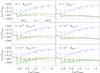 |
Fig. 11 Same as Fig. 6 except for Model A′. |
| In the text | |
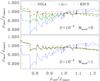 |
Fig. 12 Same as Fig. 6 except for Model B. |
| In the text | |
|
Fig. 13 Inversion results for Model A, using the same modes as in Fig. 6 but with various erroneous mode identifications, as indicated in the panels. In all panels, β = 10-8, θ = 10-4 and Msurf = 0. |
| In the text | |
|
Fig. 14 Inversion results for Model A for two similar sets of modes (see text for details). The parameters used in these inversions are β = 10-8, θ = 10-4 and Msurf = 0. |
| In the text | |
|
Fig. 15 Kernels of the n = 1, ℓ = 4 mode for Model A (lower panels) and the worst model (upper panels). |
| In the text | |
|
Fig. 16 Mean density estimates for α Cen B. The SOLA parameters are β = 10-8 and θ = 10-2, and Msurf is indicated in the panels. The vertical triple-dot-dashed line corresponds to the minimum and maximum mean densities from Kjeldsen et al. (2008). |
| In the text | |
|
Fig. 17 Mean density estimates for HD 49933. The SOLA parameters are β = 10-8 and θ = 10-2. The horizontal triple-dot-dashed lines represent the solutions from Creevey & Bazot (2011) and Kallinger et al. (2010), in the same order as in Table 8. |
| In the text | |
|
Fig. 18 Mean density estimates for HD 49933 using swapped ℓ identifications. The SOLA parameters are β = 10-8, θ = 10-2 and Msurf = 1. The solutions from Creevey & Bazot (2011) and Kallinger et al. (2010) are represented as triple-dot-dashed horizontal lines. |
| In the text | |
|
Fig. 19 Mean density estimates for HD 49385. The SOLA parameters are β = 10-8, θ = 10-2 and Msurf = 0. The horizontal triple-dot-dashed lines correspond to the best-fitting models from Deheuvels & Michel (2011). The circled results (upper panel) were obtained for pre-main-sequence models (for clarity, these are not circled in the lower panel). |
| In the text | |
Current usage metrics show cumulative count of Article Views (full-text article views including HTML views, PDF and ePub downloads, according to the available data) and Abstracts Views on Vision4Press platform.
Data correspond to usage on the plateform after 2015. The current usage metrics is available 48-96 hours after online publication and is updated daily on week days.
Initial download of the metrics may take a while.