| Issue |
A&A
Volume 539, March 2012
|
|
|---|---|---|
| Article Number | A32 | |
| Number of page(s) | 13 | |
| Section | Interstellar and circumstellar matter | |
| DOI | https://doi.org/10.1051/0004-6361/201117818 | |
| Published online | 22 February 2012 | |
XMM-Newton observation of 4U 1820-30
Broad band spectrum and the contribution of the cold interstellar medium
1
SRON, Netherlands Institute for Space Research,
Sorbonnelaan, 2,
3584 CA
Utrecht,
The Netherlands
e-mail: This email address is being protected from spambots. You need JavaScript enabled to view it.
2
Astronomical Institute, Utrecht University,
PO Box 80000, 3508 TA
Utrecht, The
Netherlands
3
Max-Planck-Institut für extraterrestrische Physik,
Giessenbachstr. 1, 85748
Garching bei München,
Germany
4
Kapteyn Astronomical Institute, University of
Groningen, Postbus
800, 9700 AV,
Groningen, The
Netherlands
5
Sterrenkundig Instituut Anton Pannekoek, University of
Amsterdam, Science Park 904, PO Box
94249, 1090 GE
Amsterdam, The
Netherlands
Received: 3 August 2011
Accepted: 16 December 2011
Abstract
We present an analysis of the bright X-ray binary 4U 1820-30, thet is based mainly on XMM-Newton-RGS data, in addition to complementary data from XMM-Newton-EPIC-pn, INTEGRAL, and Chandra-HETG, to investigate different aspects of the source. The broad band continuum is fitted well by a classical combination of black body and Comptonized emission. The continuum shape and the high flux of the source (L/LEdd ~ 0.16) are consistent with a “high state” of the source. We do not find any significant evidence of iron emission at energies ≥ 6.4 keV. The soft X-ray spectrum contain a number of absorption features. Here we focus on the cold and mildly ionized gas. The neutral gas column density is NH ~ 1.63 × 1021 cm-2. The detailed study of the oxygen and iron edge reveals that those elements are depleted, which is defined here as the ratio of the dust to the total ISM cold phase, by a factor 0.20 ± 0.02 and 0.87 ± 0.14, respectively. Using the available dust models, the best-fit points to a major contribution of Mg-rich silicates, with metallic iron inclusion. Although we find that a large fraction of Fe is in dust form, the fit shows that Fe-rich silicates are unlikely to be present. The measured Mg:Fe ratio is 2.0 ± 0.3. Interestingly, this modeling may provide additional support for a well studied dust constituent (GEMS), which is sometimes proposed as a silicate constituent in our Galaxy. Oxygen and iron are found to be slightly over- and under-abundant, respectively (1.23 and 0.85 times the solar value), along this line of sight. We also report the detection of two absorption lines, which are tentatively identified as part of an outflow of mildly ionized gas (ξ ~ −0.5) at a velocity of ~1200 km s-1.
Key words: astrochemistry / X-rays: binaries / dust, extinction / X-rays: individuals: 4U 1820-30
© ESO, 2012
1. Introduction
The interstellar medium (ISM) in the plane of our Galaxy is a dynamic and complex environment that is composed of mainly neutral matter in both gas and dust form and a warmer gas phase in the form of diffuse emission in, and above, the Galactic plane. The properties of the cold phase in the diffuse ISM have been extensively studied at long wavelengths, from the far-infrared to the far-UV (e.g. Draine 2003,for a review). A sizeable fraction of the cold phase is locked up in dust grains (e.g. Savage & Sembach 1996; Jenkins 2009,and references therein). Amorphous silicate materials together with graphite and policyclic aromatic carbon should account for the majority of the depleted elements measured in the ISM, namely C, O, Fe, Mg, and Si (e.g. Weingartner & Draine 2001; Wooden 2008). One of the major spectroscopic signatures of the presence of Fe- and Mg- rich amorphous silicates is the 10 μm emission feature. Extensive studies of this feature lead to the conclusion that the Fe:Mg ratio should be approximatively 1 (e.g. Li & Draine 2001). The main sources of both Mg and Fe silicates are O-rich asymptotic giant branch stars (AGB) and supernovae. However, the process of amorphization of the dust agglomerates, for instance by rapid cooling of the gas phase (Wooden et al. 2005) or cosmic ray bombardment (Carrez et al. 2002), strongly promotes the survival of Mg silicates. A recent analysis successfully models the 10 μm feature in terms of Mg-rich silicates, if non-spherical grain shapes are used (Min et al. 2007). Glassy material, consisting of Mg-rich silicates with metallic iron and sulfide inclusion (called GEMS, Bradley 1994), have also been commonly found during the Stardust mission. Their origin is mostly the interplanetary environment (e.g. Keller & Messenger 2004), but a fraction have a composition compatible with an ISM origin (Keller & Messenger 2008). Iron is however a highly depleted element (70–99% of Fe is in dust; Wilms et al. 2000; Whittet 2003), whose inclusion into solid grains is not completely understood (e.g. Whittet 2003). This is mainly due to the difficulty in modeling iron emission, which does not display any readily identifiable feature in long-wavelength spectra.
The abundances of the most important metals in the Galactic disk smoothly decrease with galactocentric distance. The average slope of the distribution is ~0.06 dex kpc-1 (Chen et al. 2003,and references therein). However, a large scatter in the abundance measurements as a function of the Galactic radius is reported. This is attributed to different factors that contaminate the smooth mixing caused by the pure stellar evolution process. The medium can indeed be locally influenced by e.g. supernovae ejecta, and in-falling metal-poor material into the disk (Lugaro et al. 1999; Nittler 2005).
It has become clear that the X-ray band could provide an excellent laboratory to study the silicate content of the diffuse ISM, as the absorption K edges of O (E = 0.538 keV), Mg (E = 1.30 keV), and Si (E = 1.84 keV) together with the Fe LII and LIII edges (0.71 and 0.72 keV, respectively) fall in the low-energy X-ray band. The method used is to study the absorbed spectrum of bright X-ray binaries, located in different regions in the disk, observed with high-energy resolution instruments. This allows us to probe the interstellar dust (ID) content in a variety of environments, with different extinctions and possibly different dust formation histories. Previous studies of X-ray spectra taken along different lines of sight led first to the recognition that not only gas but also dust plays a role in shaping the iron and oxygen edges (Takei et al. 2002; Kaastra et al. 2009) and later led to the quantitative modeling of those edges (Lee et al. 2009; de Vries & Costantini 2009; Pinto et al. 2010). There is not yet a clear picture of the chemical composition of the ID as seen in X-rays. Silicates containing andratite (iron-rich silicates) were reported, studying the oxygen edge of GS 1826-238 (Pinto et al. 2010), while iron oxides rather than iron silicates were reported along the line of sight to Cyg X-1 (Lee et al. 2009). This may indicative of a chemically inhomogeneous distribution of ID.
4U 1820-30 is an extensively studied source, by virtue of its extraordinary intrinsic properties. It is an ultracompact (orbital period 11.4 min, Stella et al. 1987) X-ray binary consisting of a neutron star and a He white-dwarf (Rappaport et al. 1987). The presence of X-ray bursts associated with the neutron star was recognized at an early stage (first by Grindlay et al. 1976). 4U 1820-30 is classified as an atoll source (Hasinger & van der Klis 1989) that displays kilohertz quasi-periodic oscillation at different frequencies in its power spectrum (e.g. Smale et al. 1997; Zhang et al. 1998).
The broad band spectrum has been studied with several instruments. The source displays a Comptonized continuum and a soft black-body component (e.g. Sidoli et al. 2001).
With the advent of high resolution spectroscopy, the low-energy X-ray spectrum has also revealed interesting features. Absorption by ionized ions has been reported in several studies (Futamoto et al. 2004; Yao & Wang 2005; Juett et al. 2006; Cackett et al. 2008a). The absence of a blueshift in the lines of this gas and a lack of variability generally points to an interstellar origin (but see Cackett et al. 2008a). The hypothesis of a gas intrinsic to the source is intriguing as other X-ray binaries often display absorption by ionized gas either in the rest frame of the source (van Peet et al. 2009) or outflowing away from the source (e.g. Miller et al. 2006; Neilsen & Lee 2009). The source has also been used as a backlight to illuminate the interstellar dust along the line of sight. This results in a dust scattering halo, which in this source is moderate (~3.2% at 1 keV, Predehl & Schmitt 1995), given the relatively low Galactic column density (NH ~ 1.63 × 1021 cm-2, this study).
Absorption by cold interstellar dust has been never studied in detail in this source. In this paper, we aim to perform a comprehensive view of the cold absorbing medium along the line of sight to this source. This study is based on the combined information provided by the Chandra and XMM-Newton high resolution instruments, which allowed us to meaningfully study both the Fe L and O K edges. In addition, we used dust models updated with the latest laboratory measurements (e.g. Lee et al. 2008, 2009). We also present the broad-band continuum behavior underlying the absorption features.
The adopted protosolar abundances follow the prescription given by Lodders & Palme (2009) and discussed in Lodders (2010). The broad-band energy spectrum (EPIC-pn and INTEGRAL) was fitted using the χ2 minimization method, taking care that at least 20 counts per bin are present in each data set. For the high resolution spectra (RGS and Chandra-HETG), the Cash statistic was used1. The errors quoted are for the 68% confidence level, corresponding to either Δχ2 = 1 or ΔC2 = 1. The spectral fitting package used in this paper is SPEX2 (Kaastra et al. 1996). The adopted distance is 7.6 kpc (Kuulkers et al. 2003). The nominal hydrogen column density toward the source is 1.29 × 1021 cm-2 (Kalberla et al. 2005), to be compared with 1.52 × 1021 cm-2 (Dickey & Lockman 1990).
This paper is organized as follows. In Sect. 2, we illustrate the data handling for the different instruments used. Section 3 is devoted to the continuum determination using EPIC-pn and INTEGRAL data. In Sect. 4, we describe in detail the modeling of the different absorption components using RGS and Chandra-MEG data. The discussion can be found in Sect. 5 and the conclusions in Sect. 6.
2. The data handling
2.1. Epic-pn
4U 1820-30 was observed by XMM-Newton for 41 ks on April 2, 2009 (revolution 1706). The data reduction was performed using SAS (ver. 9.0). The EPIC-pn (Strüder et al. 2001) was operated in full-frame masked mode. In this mode, the central 13 × 13 (in RAW coordinates) pixels are flagged as bad on board, masking the central part of the PSF. The full-frame mode was chosen to optimally study the halo of diffuse emission surrounding the source, which was caused by the scattering of the intervening dust along the line of sight. However, the spectrum of the central source is recovered from the so-called Out of Time (OoT) events, which are the photons trailed through the detector during the read-out of the frame. The exposure time of the OoT events is 6.3% of the total exposure. We extracted the source spectrum from the RAW coordinate event file. We selected 11 columns from RAWX 32 to RAWX 42, avoiding the central 2 columns, which were affected by pile up. We selected RAWY <89 to avoid the innermost region of the PSF, which was still affected by pile up or X-ray loading3.
The background was selected in a neighboring region. The exposure time of the background was scaled to match the effective exposure of the OoT events. Given the brightness of the source, the nominal background contribution was modest. However the whole area was contaminated by the photons of the scattering halo, which have a different distribution depending on the position in the detector. The OoT events were extracted from a modified event file processed in such a way that the charge transfer inefficiency (CTI) corrections were not applied and all the photons were assumed to originate from the central source coordinates.
2.2. RGS
Owing to the brightness of the source, some RGS (den Herder et al. 2001) portions of the grating data were affected by pileup. In addition, in RGS2 the high number of events per CCD frame (twice the exposure time compared to RGS1, because of the single node readout) tended to fill up the buffers too rapidly. Limits on the data handling in relation to telemetry prevented the buffers from being cleared in time, leading to data losses for some CCDs. A method for recognizing the spectral regions unaffected by pile up is to compare the first and the second order for each grating. Calibration shows that in the absence of pile up, the ratio of the spectra of the two orders, in the region where they overlap, should be unity4. In Fig. 1, we show the ratio for RGS1. We see that the maximum pile up is recorded between 14 Å and 19 Å, where the effective area of RGS is the largest. In this region the ratio is about 1.1, which corresponds to only a 6–7% pile up. In RGS2, the ratio of the 2nd to 1st order even reaches a value of five in selected regions. At longer wavelengths (λ > 20 Å), the combined effect of absorption and decrease in the effective area significantly lowers the count rate. Therefore, this region is unaffected by pile up and can be safely used. Absorption features are however in general minimally influenced by this effect. We have chosen to keep the useful data given by RGS2 around the iron L edge, with care of locally fitting a different continuum for RGS1 and RGS2, using “sectors” in SPEX, as defined below (Sect. 4).
We also used archival RGS data (Table 1) in order to improve the signal-to-noise ratio (S/N). This observation displayed a short period of flaring background, which was filtered out. This resulted in a cut of 3 ks on the total exposure time.
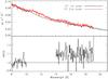 |
Fig. 1 Upper panel: comparison of the second and first order for RGS1. Lower panel: the ratio of the second to the first order provides an indication of pile up in the spectrum. |
2.3. Chandra-HETG
To increase both the S/N and energy resolution at wavelengths ≲18 Å, where the Fe, Mg and Si edges stand, we considered archival Chandra-HETG data, selecting the higher-flux data sets available (Table 1). We obtained the final products, processed in April 2010, from the TGCat archive5. The three observations displayed similar fluxes and continuum parameters, therefore we combined the data, separately for the HEG and the MEG arms. The HEG data are of low S/N at wavelengths longer than ~17 Å. In the following, we refer only to the MEG data, unless otherwise specified.
2.4. INTEGRAL
To constrain the continuum spectrum of 4U 1820-30 across an as-large-as-possible energy band, INTEGRAL data can be very useful. Fortunately, the Galactic center region was observed by INTEGRAL for ~73 ks from March 30, 2009 to March 31, 2009 during satellite revolution 789, and for ~38 ks on April 3, 2009 during revolution 790. The XMM observation ended during the latter observation. We can therefore assume that these INTEGRAL observations are quasi-simultaneous with the XMM-observation. 4U 1820–30 was in the field of view of the INTEGRAL Soft Gamma-Ray Imager ISGRI (15–300 keV; Lebrun et al. 2003) at source angles smaller than  for all 21 individual pointings (so-called science windows) of the rev. 789 observation and all ten pointings of rev-790. The source was outside the field of view (
 diameter zero response) of the Joint European Monitor for X-rays JEM-X (3–35 keV; Lund et al. 2003) during the rev. 789 observation, but within the field of view during four individual pointings of rev. 790.
We generated mosaic maps for ten logarithmically spaced energy bands across the 20–300 keV range for the ISGRI rev. 789 observation using OSA version 9.0 (distributed by the ISDC; Courvoisier et al. 2003) imaging tools. We checked these maps for significantly detected sources and subsequently derived spectral information for all these sources in 13 pre-defined energy windows across the 13–520.9 keV energy range.
For JEM-X (telescope 1), we followed similar imaging and spectral extraction procedures yielding spectra of 4U 1820-30 in 16 pre-defined energy bands across the 3.04–34.88 keV.The observation log is displayed in Table 1.
The multi-instrument observation log for 4U 1820-30.
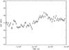 |
Fig. 2 Light curve of EPIC-pn data as selected in Sect. 2.1. Note that the displayed count rate cannot be used to recover the flux of the source. The bin time is 500 s. |
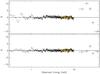 |
Fig. 3 Upper panel: residuals to a simple absorbed power law for EPIC-pn and INTEGRAL data. JEMX data have been highlighted for clarity. Lower panel: residuals to the best fit consisting of a black body plus Comptonized emission, modified by both a neutral and ionized absorbing material. EPIC-pn data have been rebinned for display purposes. |
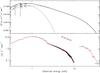 |
Fig. 4 Upper panel: the best-fit model consists of a black body (dashed line) plus Comptonized emission (dot-dashed line), modified by both a neutral and ionized absorbing material (Table 2). Lower panel: best-fit model superimposed on the EPIC-pn, JEMX and ISGRI spectra. |
3. The broad band spectrum
We first extracted the light curve from the EPIC-pn OoT events as described in Sect. 2.1, thus the resulting count rate could not be used to recover the absolute flux. The 0.5–10 keV light curve is shown in Fig. 2, using a bin size of 500 s. It shows a modest variation of at most 13% during our observation. The rates in the soft (0.5–2 keV) and the hard (2–10 keV) band followed the same pattern.
We fitted the EPIC-pn and INTEGRAL spectra simultaneously. The source was caught at a relatively high flux, with a 2–10 keV flux of ~5.0 × 10⁻⁹ erg cm-2 s-1 (Table 2). In Fig. 3 (upper panel), we show the residuals with respect to a simple powerlaw with photoelectric absorption. From the residuals, we see a complex spectrum at energies below 1 keV, which is probably produced by ionized absorbing gas. The spectrum is clearly detected up to 40 keV.
As a simple powerlaw is not an acceptable model (χ2/ν = 2412/1724 = 1.39, where ν is the number of degrees of freedom), we first added a black body component, to mimic the often observed soft energy emission (χ2/ν = 2273/1722 = 1.32). This is parameterized by the black-body temperature (Tbb) and its normalization. However, a black body plus power law model fails to explain the spectral curvature seen at high energies. We then substituted the powerlaw model with a Comptonization model (COMT model in SPEX; Titarchuk 1994), where the parameters are the temperature of the seed photons (kT0) and the optical depth of the electron cloud (τ) where the photons are Compton scattered to the final temperature (kT1). This model provides a satisfactory fit to the broad-band continuum (χ2/ν = 1756/1720 = 1.02; see Fig. 3, lower panel, Fig. 4, and Table 2).
We repeated the fits using a disk black body model (i.e., emission from a standard Shakura-Sunyaev disk, model DBB in SPEX) instead of a simple black body. We did not obtain an equally good fit using DBB either in addition to a simple powerlaw model (χ2/ν = 2302/1722 = 1.33) or DBB plus Comptonization (χ2/ν = 1998/1720 = 1.16).
Broad band modeling of the source using EPIC-pn and INTEGRAL data.
In the 6.4 keV region, there is no clear evidence of iron emission lines. A 3σ upper limit of 25 eV to the equivalent width is obtained if a delta line is located at a fixed energy of 6.4, 6.70, and 6.97 keV, respectively. We also searched for a relativistically modified line profile (LAOR model in SPEX; Laor 1991). In this model, the line arises from the accretion disk where the intensity follows a R−q profile, where R is the distance of the disk gas from the source. Leaving the energy as a free parameter did not lead to a meaningful fit. We then fixed the energy of the line to 6.97 keV, following previous studies of 4U 1820-30 (e.g. Cackett et al. 2010). The best fit reproduces a very broad, but weak line profile, with parameters q = 2.8 ± 0.2 and i < 14°, where i is the disk inclination. The flux of the line is (1.6 ± 0.7) × 10-4 photons cm-2 s-1.
The complex absorption at soft energies was modeled following the prescription given by the high-resolution data (Sect. 2.2). We therefore added a minor contribution from ionized absorbers ( cm-2) and the Galactic neutral absorber, which contributes to most of the low-energy curvature. We note that the best fit neutral column density is about 40% lower than the best-fit obtained in the RGS analysis. This may be caused by foreground scattering halo soft-emission (observed for the full exposure) located just in front of the OoT event (observed for 6.3% of the exposure time) that remains after the subtraction of the local background. The scattering halo appears as diffuse emission that extends on top of both the wings of the point spread function of the source and the OoT events themselves (e.g. Predehl & Schmitt 1995; Costantini et al. 2005). The scattering process is strongly energy dependent (Mathis & Lee 1991). In particular, the halo is brighter at softer energies. The net effect is therefore to add more photons to the soft energy spectrum of the OoT events, reducing the measured absorption toward the source. This effect appears to be even more enhanced by the reduction in the OoT absolute flux caused by the cut of the central two columns, where most of the source photons are.
4. The high resolution spectrum
Since the energy band of the RGS is insufficient to discriminate among different broad-band models, we adopted the model defined in the previous section. The spectrum contains evident O i K and Fe i L edges, caused by the absorption of neutral material. In addition, absorption by ionized gas is highlighted by the O viii, O vii, and O vi absorption lines.
We used a collisionally ionized plasma model (model HOT in SPEX), with a temperature frozen to kT = 5 × 10⁻⁴ keV, in order to mimic a neutral gas. This model fits to first order the edges and resonant lines from the neutral species, leaving however noticeable residuals in the fit. To extract more robust results from the absorbtion features, we added archival RGS (Sect. 2.2) and Chandra-MEG data (Sect. 2.3). As these data sets were obtained at different epochs, the continuum shapes may differ significantly. To bypass this complication, we used the “sectors” option in SPEX6 and we allowed the continuum parameters to vary freely for each sector. The RGS1 and RGS2 data derived from the recent observations were treated as different data sets (thus with different continua), as the RGS2 broad band shape was affected by pileup. The parameters of absorber components were coupled together for all the data sets.
4.1. The ionized gas
The RGS spectrum of 4U 1820-30 displays narrow absorption features from ionized gas, mainly from oxygen, iron, and neon. In particular, Ne ix and O vi–O viii are prominent features of this gas. For this fit, we ignored the data below 13 Å for RGS. In this region there are some wiggles in the local continuum, which are mainly caused by pile up, could add uncertainties to the determination of the absorption parameters. Here we focused on the neutral or mildly ionized phase of the ISM. Therefore, we simply modeled the higher ionization lines with a phenomenological model (SLAB in SPEX), which calculates the transmission from a thin layer of gas. We deferred a more detailed analysis of this gas component to a future publication. The resulting ionic column densities of the main ions, as measured by RGS, are reported in Table 3. Following Yao & Wang (2005), we assumed a velocity broadening of σv = 62 km s-1. All subsequent fits in the present analysis already take into account this highly ionized component.
Parameters of the main lines of the more ionized ions as measured by RGS.
Parameters for the oxygen edge modeling.
4.2. The oxygen edge
The oxygen edge at 0.538 keV was fitted using the high quality data of the two RGS epochs for the wavelength range 19−36 Å. The neutral material, modeled by a low temperature (kT = 5 × 10⁻⁴ keV) in a collisional ionization equilibrium, closely fits the long wavelength curvature produced by the ISM absorption as well as the O i 1s–2p absorption line at 23.5 Å (Fig. 7). The edge shape appears to be modified by several sharp absorption features. Some of them can be easily identified with the O vii and O vi lines, which belong to a highly ionized phase (Sect. 4.1). At the shorter wavelength side of the O i line, we see O ii at λ = 23.35 Å and also weaker O iii and O iv lines. Two absorbers with different temperatures were required to fit these lines (Table 4, Col. (1)). The reported line widths were automatically evaluated in SPEX using a curve of growth analysis applied to multiple lines belonging to the same absorption system (e.g. Spitzer 1978). This allowed us to accurately evaluate the line width using basic parameters such as the ionic column density and equivalent width. In this case, O i, Fe i, and N i transitions were used to model the cold gas (comp 1 in Table 4). The strongest transitions were found to be saturated, which in principle might have introduced additional uncertainty in determining the line width. However, as shown in Fig. 5, for the lines we study here, the ionic column density as a function of the line equivalent width depends marginally on the velocity width. This behaviour of the curve of growth is due to the large a-Voigt parameter for the inner-shell transitions (Mihalas 1978; Kaastra et al. 2008, for a full discussion). We note that the nitrogen region was not modified by dust and the line widths were then easier to evaluate. In addition, many of the the weaker transitions of the same neutral ions are not saturated. For the kT ~ 3.2 eV gas (comp 2), O ii, Fe ii, and N ii are among the strongest ions. These are relatively weaker lines where saturation does not play a major role. The relatively limited resolution of the instrument does not allow us to distinguish multiple velocity-width components within a same absorption line. Therefore, we consider here the total ionic column density along this line of sight.
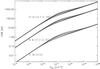 |
Fig. 5 Line equivalent width as a function of the ionic column density for O i, N i and O ii. The velocity dispersions are σv = 10, 100, 200 km s-1. Curves of different ions have been shifted for clarity. |
Dust should also be present along this line of sight, as 4U 1820-30 is known to display a dust scattering halo (Predehl & Schmitt 1995) that is also clearly evident in the present EPIC-pn data. We therefore fitted the oxygen edge by adding the AMOL model in SPEX. We considered 16 oxygen compounds for this analysis (see Appendix A). This list includes silicates and oxides that are common in the ISM and some lighter (also icy) materials. Absorption features produced by dust, in contrast to gas, are smooth and broadened. All the oxygen compounds considered here have no appreciable effect at λ ≲ 23.7 Å (Fig. A.1).
Below we describe a simple fit using a single dust component at a time, adding a second component if the fit requires it. This makes the description of the model and the required steps to perform the final best-fit solution simpler to follow. This approach is however the result of a rigorous fitting procedure for both the oxygen and iron edges, which is fully described below (Sect. 4.4).
We first attempted to fit the whole spectral region assuming that it was affected only by dust absorption. In the fit, we allowed the hydrogen column densities of the gas producing O i and O ii (comp 1 and 2 in Table 4) to vary as free parameters. We also defined the abundance of oxygen in the cold phase (comp 1) as a free parameter, to help balance the amount of oxygen locked up in dust. In this model, we suppressed the gas component (comp 3) that mainly produces O iii (λ = 23.07 Å), as this line is the main absorption structure in the region where dust also plays a major role. It is clear that fitting the region around 23 Å only in terms of dust remarkably worsens the fit. The range of values for which the fit is poorer is indeed ΔC2 = 35−180, depending on the compound, for Δν = 2, with respect to the pure gas modeling. This indicates that not only dust absorbs radiation in the ~22.7–23.1 Å region. In Fig. 6, upper panel, we show the oxygen region where the pure gas fit is compared with the fit with MgSiO3 (dashed line) or Mg1.6Fe0.4SiO4 (olivine, dashed-dotted line), suppressing comp 3.
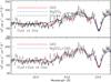 |
Fig. 6 Fits in the oxygen region. Here only RGS1 of the most recent observation is displayed for clarity. Upper panel: comparison between a fit only in terms of gas (solid line) and the best fit obtained using dust (dashed line). For comparison an unacceptable fit using olivine (dashed-dotted line) is also displayed. Lower panel: comparison between a fit only in terms of gas (solid line) and the best fit obtained with a mixture of gas and dust (dashed line). See more details in the text. |
Finally, we included both the kT ~ 13 eV gas absorption (comp 3) and dust absorption (Table 4, Col. (2)). The improvement to the fit was then ΔC2 = 10−108 for Δν = 1. The inclusion of most of the individual dust components improved the fit. However, we could identify two compounds for which the improvement to the fit was the largest (ΔC2 = 105−108). These are H2O, in the form of crystal or amorphous ice, and MgSiO3. In Fig. 6 (lower panel), we show how a fit with pure gas and a gas+MgSiO3 mixture (comp 5 in Table 4) compare with each other. We note that a fit using H2O is indistinguishable in practice from MgSiO3 as the spectral feature is very similar (Fig. A.1, Sect. 4.4 for discussion). Interestingly the compounds with both oxygen and iron provided the least improvement (if not a worsening) of the fit. In particular, the fit rules out the most complex aggregates of oxygen and iron (e.g. magnetite, franklinite, olivine, and almandine; see Fig. A.1 for the chemical composition).
As noted above, none of the dust compounds considered here have features below 23.7 Å. However, from Fig. 6 we note two clear absorption features (present in both RGS data sets) at ~22.3 Å and 22.65 Å (marked with arrows) detected with 6.8σ and 3.8σ significance, respectively. These features do not belong to the ionized absorber producing the O vii line (Sect. 4.1), but to a lower ionization gas. We tentatively fitted these features with a photoionization model (XABS in XSPEC), obtaining a low column density (NH ~ 4.3 × 1019 cm-2) and an ionization parameter7 logξ ~ −0.5 (comp 6 in Table 4). Interestingly, the two major lines, identified as O iv and O v show a systematic blue-shift of about −1200 km s-1 (Table 4, Col. (3)). From the absorber model, we note that the other lines predicted using these parameters fall either in a lower-resolution and noisier part of the spectrum (e.g. lines of iron) or where the spectrum is heavily absorbed by the neutral gas (e.g. nitrogen lines).
The best fit to the oxygen edge region, including RGS data sets taken in two epochs is displayed in Fig. 7.
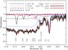 |
Fig. 7 Best fit transmission spectrum (Table 4, Col. (3)) in the oxygen edge region. This allows to compare absorption at different epochs, removing the contribution of the continuum. The upper curves display the transmission of the various absorbing components. Note that for clarity only absorption by oxygen is displayed (i.e. no hydrogen absorption). Data have been rebinned for clarity. |
 |
Fig. 8 Detail of the iron L edge region. Here for clarity we display only the MEG and a displaced RGS2 data set. The best fit (solid line, see Table 5) is compared with pure gas fit with solar abundances (dotted line) and with a mixture of gas and iron-rich olivine (thick solid light line). |
4.3. The iron L edge
In Fig. 8, a fit to the Fe LII and LIII edges in terms of absorption by pure gas with solar abundances is shown (dotted line). In this fit two RGS epochs and the MEG data sets were used. We found a clear mismatch not only of the depth, but also the position of the LII and LIII edges. We note that in the fit to the iron edges, it is essential to include the higher resolution MEG data (Fig. 8). A straightforward way to improve the fit is to modify the iron abundance. By allowing this parameter to vary, we obtained a reasonable fit, although the position of the edge in the model did not match the data. In this case, the abundance of iron, assuming that the absorption is only in the gas phase, is about 0.37 times the solar one. However, absorption by dust is known to alter the LII/LIII ratio and to shift the position of the edge with respect to absorption by gas (see e.g. Lee et al. 2009). For the fitting, we considered the compounds measured by Lee et al. (2009), namely metallic Fe, hematite (Fe2O3), lepidocrocite (FeO(OH)), fayalite (Fe2SiO4), and iron sulfate (FeSO4). These transmission models were implemented in the AMOL model in SPEX. As for the modeling of the oxygen edge, we first followed a rigorous approach (Sect. 4.4), which in turns justified the simpler approach described here, i.e. fitting the dust components one by one, together with the gas model. In the latter, the iron abundance was a free parameter. This procedure provided a measure of the depletion of the gas phase. On the goodness-of-fit basis, the single dust compound that most accurately models the data is metallic iron (Table 5). We then tried all possible combinations of gas and two dust components. We only found a marginally significant presence of Fe2O3, in addition to the metallic iron component (Table 5, Fig. 8, solid line). Hematite (Fe2O3) is a compound for which both iron and oxygen edges’ dust profiles are implemented in the AMOL model. We therefore tested the presence of this compound in the oxygen edge region, obtaining an upper limit to the column density that is consistent with the value obtained in the iron region. In Fig. 8, we also compare the best-fit model with a model for an iron rich olivine (fayalite, Fe2SiO4), which does not provide a good fit (Table 5). This suggests that fayalite cannot have a major contribution to the absorption here. We could not test the same kind of olivine as for the oxygen edge (Mg1.6Fe0.4SiO4) as at present no laboratory measurement of this compound at the iron L edge is available. In Fig. 9, the best fit is shown where data from both RGS and Chandra-MEG are displayed. The spectra were normalized to their continuum shape for display purposes. We also normalized the spectra to the total hydrogen column density so that only absorption by iron was visible for the neutral phase. Along with the best fit (solid line), the different contributions are shown for atomic gas (dotted line), metallic iron, and Fe2O3 (light dash-dotted lines). In addition, the contribution of the ionized gas to the spectrum is shown with a dashed line (e.g. O vii line at 17.76 Å).
Despite the significant improvement to the fit with respect to a gas-only model, the iron edge is clearly more complex that our parameterization. In particular, positive residuals are present at the longer wavelength side of the edge. This effect was found previously using different instruments (Kaastra et al. 2009; Lee et al. 2009).
Goodness of fit for the iron edge models.
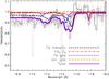 |
Fig. 9 Best-fit transmission spectrum of the region around the iron LII and LIII edges. This allows us to compare absorption at different epochs, removing the contribution of the continuum. The upper curves display the transmission of the various absorbing components. |
4.4. Further insight into the Fe L and O K edge fitting
The modeling of photoelectric edges modified by dust absorption requires some caution, as in principle many components can contribute to the edge shape, which is in turn smeared, in contrast to the atomic transition features, which are very sharp and relatively easy to identify. Therefore, the accuracy of the result depends on the resolution of the instruments, the S/N, the completeness of the dust models, and finally on how many independent parameters there are in the problem.
In this study, we combined the higher resolution of Chandra-MEG data with the sensitivity of RGS to study the Fe L edges. For the oxygen edge, we used the high quality RGS data, as the Chandra-HEG effective area dramatically drops in that spectral region. 4U 1820-30 is also a high flux source, absorbed by a gas and dust column density that is optimal for studying the O and Fe edges.
The dust edge profiles that we used in our study are a collection of what is available in the literature up to now (e.g. Barrus et al. 1997; Parent et al. 2002; van Aken et al. 1998; Lee et al. 2008, 2009). This database is not complete, but the main representatives of oxides and silicates for both oxygen and iron are present (see Appendix A, Lee et al. 2009). This is sufficient for a first order analysis.
The simultaneous analysis of two edges produced by dust along the same line of sight allowed to cross-validate our results. In addition, common knowledge of both the abundances and physical conditions in the ISM allowed us to place further constraints on the edge fitting. Here we illustrate this in detail.
In the ISM, a mixture of chemical compounds exists. We tried to simulate this by mixing all possible combinations of edges profiles available for a given edge. The AMOL model allows to fit four different components at a time. We therefore had for each edge a number of fits n where n = nd ! /4 ! (nd − 4) ! and nd is the number of available edge’s profiles. Examining the output we note that the combinations that improve the fits were those with either one or two components, for which the remaining column densities are zero. If two components were adopted, one strongly dominated over the other, whose relative value was never more than 20%. This applied to both the oxygen and the iron edge. This justified the simplified way of illustrating the fitting used in Sects. 4.2 and 4.3 above.
We further analyzed all fits that were within 3 sigma of the best-fit values shown in Sects. 4.2 and 4.3. Interestingly, for both iron and oxygen, no models containing iron-rich silicates were among these selected models.
For iron, we could rule out models, within the “3 sigma” set, containing hematite (Fe2O3) with a total molecular column density8 larger than 4.4 × 1015 cm-2. This resulted from the cross-validation we performed with the oxygen edge, as for hematite we have both the O and Fe dust profiles. Indeed, none of the “3 sigma” models for oxygen contained this compound. We therefore added it to the oxygen edge best-fit model, obtaining the limit above (and compatible with that found for the iron edge best-fit, see Sect. 4.3).
We could also rule out the “3 sigma” models containing Fe2S2 as in this case the fit inferred an amount of sulfur that is ~3.8 times solar. In this case, the sulfur edge would have been significantly enhanced, but this is not evident in our data.
For the oxygen edge, this multicomponent fitting pointed very clearly to a predominance of MgSiO3 in all the “3 sigma” set. As noted in Sect. 4.2, a similarly good fit is obtained if water ice is the predominant component owing to the very similar edge profiles of the two compounds (Fig. A.1). However, we could readily rule out this option, as along the line of sight of 4U 1820-30 the bulk of cold material is a diffuse interstellar medium, where water is virtually absent and silicates are in contrast abundant (e.g. Wooden 2008).
4.5. The magnesium and silicon edges
The Mg K and Si K edge (at 9.47 and 6.723 Å, respectively) were analyzed using the combined information derived from Chandra-HEG and MEG data, which provides in this band a higher energy resolution. In the case of Si, the energy of the edge is also outside the RGS range. The quality of the data and the relatively low Galactic column density hampered any detailed characterization of the edges. We used the auxiliary information provided by the oxygen edge fitting (Sect. 4.2) to which a model including MgSiO3 provided the closest fit. For that compound, we benefited from the laboratory measurements of both the O and Si edges. For Mg, for which we did not have any measurement, the relative column density was included in the model in the form of an artificial gas-shaped edge. We therefore added to the gas absorption model this specific dust component, fixing the amount of magnesium and silicon locked in dust and defining the amount of Mg and Si in the gas phase as free parameters. This model agrees with the data, within the uncertainties. The column density of Si in dust is  cm-2, while the Si in gas is
  cm-2. Therefore, the inclusion of Si in dust is ~85% of the total neutral Si along the line of sight. For the Mg edge, we obtained a
  cm-2, while the value imposed by the oxygen fit to the Mg locked in dust was
  cm-2. The amount of Mg locked up in dust according to this model is about 96%.
4.6. The neon and nitrogen edges
To study the neon edge (λ = 14.24 Å), we used the combined data of RGS and Chandra, while for the nitrogen edge we used only the RGS data. These elements are only present in gas form in the ISM (e.g. Wilms et al. 2000). Fitting neon with our Galactic absorption model, we found a column density of 2.07 ± 0.02 × 1017 cm-2, which converted into a formal slight overabundance with respect to solar 1.2 ± 0.1.
Next to the nitrogen edge at 30.76 Å, we can also distinguish absorption by the 1s–2p line at 31.28 Å. The measured column density of nitrogen is (1.33 ± 0.01) × 1017 cm-2, corresponding to an abundance of 0.9 ± 0.1 times solar, which is consistent with the value expected using solar abundances.
5. Discussion
5.1. The broad band continuum and the iron emission line
We have analyzed the simultaneous observation of 4U 1820-30 using XMM-EPIC-pn and INTEGRAL. The fit of the continuum is consistent with black body emission plus a Comptonized component, the latter extending up to 40 keV. The source was observed in a high flux state, accreting at Lbol/LEdd ~ 0.16. We have assumed that Lbol = 2 × L(2−20 keV), where the unabsorbed luminosity L(2−20 keV) is ~3.1 × 1037 erg s-1. The Eddington luminosity for ultracompact systems is LEdd ~ 3.8 × 1038 erg s-1, following Kuulkers et al. (2003). The spectral shape is also consistent with a high state scenario. The hard energy portion of the spectrum is well-fitted by a Comptonization model with an effective cut-off at ~40 keV, which is consistent with previous observations of the source in the high-state (Bloser et al. 2000; Sidoli et al. 2001). The black body emission, which reproduces well the soft energy range of the present observation, has a temperature similar to that of the Comptonization seed photons. This may suggest that in ultra-compact X-ray binaries seed photons originate from the accretion disk (Sidoli et al. 2001).
A relatively weak or undetected iron line is a common feature of confirmed ultra-compact X-ray binaries (as defined e.g. in in’t Zand et al. 2007), similar to 4U 1820-30. This may be simply explained by the nature of the donor star in these systems. Owing to the high surface gravity (log g ~ 8), heavier elements in the white-dwarf companion sink to the internal layer of the star (e.g. Fontaine & Michaud 1979), leaving few high Z metals available for the accretion flow. In 4U 1820-30 however, a faint, variable, and relativistically smeared iron line has been reported (e.g. Cackett et al. 2008b, 2010). In our data, no narrow emission features, either from neutral or ionized iron, have been found (Sect. 3). A fit with a relativistically smeared iron line leads to a very elusive 2σ detection of the feature. The photon flux of this line is about 16 times fainter than that found in recent Suzaku data (Cackett et al. 2010).
In exceptional circumstances, such as superburst episodes, a large quantity of heavy element ashes may be ejected during the neutron star photosphere expansion. This could possibly cause detectable features (e.g. in absorption) such as iron in the X-ray spectra (in’t Zand & Weinberg 2010). In 4U 1820-30, the presence of the iron line could then be the tracer of burst activity, that is undetectable at the epoch of our observation.
5.2. The dust components
The high resolution spectrum of 4U 1820-30 shows evidence of absorption by dust, especially around the Fe L and O K edges (Figs. 7, 9). In the fits, we explored all the possible combinations of dust mixtures (Sects. 4.3 and 4.2). The best fit shows a preference for absorption by enstatite (MgSiO3), which is the end series of the pyroxene silicate mineral, metallic iron (Fe), and traces of iron oxides in the form of hematite (Fe2O3). In the modeling, 16 and 5 different compounds were considered for oxygen and iron, respectively. The set of models does not cover the whole range of possible compounds present in the ISM. However, what are commonly believed to be the main constituents (e.g. olivines, pyroxene, oxides as well as simpler compounds) in the diffuse ISM (e.g. Whittet 2003; Wooden 2008) are represented (see Appendix A, Lee et al. 2009). An additional effort to obtain new measurements has been carried out (Lee & Ravel 2005; Lee et al. 2009; and de Vries et al., in prep.). The available X-ray measurements were mostly performed on crystalline materials. Dust in the form of crystals is significantly present only in specific astronomical environments, such as comets (Wooden 2008) or the inner regions of protoplanetary disks (van Boekel et al. 2004). In the ISM, the amount of crystalline silicates, relative to amorphous grains, is <5% (Li & Draine 2001), hence we do not expect to find a sizeable amount of it in our data. However, for the handful of compounds for which X-ray laboratory measurements of both glassy and crystalline forms are available, we tested that the spectral difference is appreciable only if the resolution is of about 3–5 eV. Therefore, with the present data, our analysis using crystalline grains is a good first order approximation of the chemical composition of the ID. In the glassy form, crystalline material loses the ordinate internal structure proper of a crystal. For simplicity, although formally incorrect, we may refer to an amorphous silicate with a certain (for instance enstatite) stoichiometry, as either glassy-enstatite or glassy-MgSiO3.
5.3. Abundances and depletion
As X-ray spectra do not contain any distinctive hydrogen feature, either in emission or absorption, the total hydrogen column density was inferred from the low energy curvature of the spectrum, which extends down to 36 Å. This is a reliable method, as starting already at about 25 Å, the transmission is largely dominated by He and H. The best-fit value of the hydrogen column density is NH = (1.63 ± 0.02) × 1021 cm-2, which is slightly larger than the nominal values (1.52 ± 0.07) × 1021 cm-2 (Dickey & Lockman 1990) and (1.32 ± 0.05) × 1021 cm-2 (Kalberla et al. 2005), which are the average values over a region of 1° radius around the source. The reason for that could be that the spectral curvature measures the total amount of hydrogen (i.e. in H i, H ii, and H2 forms), which should be larger than H i alone. The amount of H2 in the diffuse ISM is relatively low (e.g. Takei et al. 2002). We estimated the amount of H ii using the O ii/O i ratio as a proxy (following the expression in Field & Steigman 1971). We found that ~4% of the measured hydrogen column density is in the form of H ii. This would reconcile our value with the H i measurement mentioned above. In addition, it could be that a small fraction (in this case no more than 1–3 × 1020 cm-2) of the total H resides in the immediate surroundings of the source, as in other sources (e.g. Predehl & Schmitt 1995; van Peet et al. 2009). Such a low column density would be insufficient, however, to produce the observed deep absorption features. We computed the following abundances taking as a reference the value we measured from the X-ray spectrum.
In the iron edge region (Sect. 4.3), a fit in terms of pure gas is clearly unacceptable. This points easily to an additional contribution from dust. According to our best fit, the total column density of gaseous iron is then  cm-2. From the iron edge fit, we obtained a total dust column density of
  cm-2. The sum of these iron components provided NFe = (4.3 ± 0.5) × 1016 cm-2. When we compared this number to the value predicted from our set of solar abundances,
  cm-2 (given the best-fit total hydrogen column density of NH = (1.63 ± 0.02) × 1021 cm-2), we found that the abundance is 0.85 ± 0.08 times solar. The depletion of iron, which is defined here as the ratio of the dust abundance to the total amount of a given element is instead 0.87 ± 0.14 (Table 6). This value is often reported to be higher (e.g. 0.97, Jenkins 2009). However, other studies report lower values of the Fe depletion (0.7, Wilms et al. 2000). We note that, considering some uncertainties that still remain in the edge fitting (Sect. 4.3) the value we obtain may be considered as a lower limit.
At a temperature of kT = 0.5 eV, Fe is mainly Fe i and only ~2% of the total iron in Fe ii. The sum of the mildly ionized phase (Fe ii–Fe iv), excluding therefore the high ionization ions described in Sect. 4.1, is 0.24 × 1016 cm-2 along this line of sight, i.e. Feion/Fe , remembering that neutral iron is ~87% depleted.
In the oxygen region, the evidence of dust is not as striking as in the iron region (Sect. 4.2). For the best fit including cold (kT = 0.5 eV) gas, the amount of oxygen in the gas form is consistent with being solar ( cm-2). However, the amount of oxygen in dust compounds is
  cm-2. The total amount of oxygen is then NO = (1.2 ± 0.1) × 1018 cm-2, representing about a 23% overabundance with respect to solar (Table 6). With this reference value, the amount of depletion is 0.20 ± 0.02. Oxygen depletion and abundances based on Chandra data were previously presented by Yao et al. (2006). As expected, the column density of O i (
 ) that we measure is similar to theirs. However, taking as a reference the Anders & Grevesse (1989) abundances (
 ), Yao et al. (2006) found an underabundance of oxygen of about 30%. In the reference list that we adopted (Lodders & Palme 2009), the absolute oxygen abundance is significantly lower (
 ).
).
Finally, the ratio of mildly ionized oxygen (O ii–O v, with total column density 5.5 × 1016 cm-2) to the total oxygen in gas form is Oion/O .
.
As shown in Sect. 4.5, the inclusion of Si in dust is 85%, while for Mg it is 97% of the total ISM. These values are comparable to those reported in the literature (e.g. 80–92% and 90–97% for Mg and Si, respectively, Wilms et al. 2000; Whittet 2003). However, Mg and Si could not be studied in detail in this case because of the relatively low column density toward 4U 1820-30, which causes the shallow absorption edges. Moreover, our fitting of the Mg and Si edges relies on the oxygen modeling. Therefore, if other Mg or Si compounds are present, they are difficult here to detect. Keeping in mind these limitations, we report the depletion values of Mg and Si in Table 6, for completeness. The abundance estimate of both Mg and Si are again driven by the oxygen edge fitting and are formally slightly above the solar values.
Relative abundances and depletion values from the present analysis.
In Table 6, we list for each element, the ratio of proto-solar abundances and the amount of depletion defined as the ratio of the dust to total ISM abundance.
An additional test of the abundances derived from the X-ray data would of course come from high-resolution (R = λ/Δλ > 20 000) UV data, where the elemental gas phase can be accurately studied (e.g. Savage & Sembach 1996). In the case of 4U 1820-30, high-resolution UV data (either from HST or FUSE) are unavailable. 4U 1820-30 was observed only with the HST-STIS-G140L spectrograph (R = 1000). We find that the S/N of the data was insufficient for a quantitative study of the absorption lines.
5.4. The location of the cold matter
It has been established that a gradient in the abundances in our Galaxy exists for the most abundant metals. An average slope of 0.06 dex kpc-1 should be roughly representative of the gradient for both O and Fe (see Sect. 1).
In our analysis, we estimated a slight overabundance of oxygen (by a factor ~1.2, see Table 6), while iron is a factor ~0.85 of the solar value. This appears to contradict with expected abundances at the distance of the source, where according to the gradient above, some overabundance is expected. However, 4U 1820-30 is located at latitude b = −7.9133°, i.e. about 1 kpc below the Galactic disk, hence our line of sight intercepts a relatively small fraction of the cold ISM near the source. The cold phase that we detected towards this source is instead due to absorption in the environment close to the Sun.
For iron, a gradient as a function of both the radial distance from the Galactic center and the height above the disk has been estimated (e.g. by Chen et al. 2003, based on open cluster measurements). Our value of [Fe/H]9 is –0.07. This is consistent, within the errors, with absorption in the disk at the distance of the Sun rather than absorption local to the source, at the height of 4U 1820-30 below the disk (Chen et al. 2003).
The location of the gas based on the oxygen abundance is difficult to determine, as there is a large scatter in the measurements (e.g. Rudolph et al. 2006,for a compilation of results). Our oxygen abundance is consistent with both absorption far from or near the observer. It is therefore not straightforward to understand where the bulk of the absorption takes place based on gradient measurements. However, a systematic analysis of dust scattering halos points out that most of the scattering (and therefore the absorption by dust) should occur within ~3° of the Galactic plane (Predehl & Schmitt 1995). This further supports the intuitive idea that most of the cold absorbing material is located close to the observer.
5.5. The silicates
In the present study, we have found that the fit to both the iron and oxygen edges is in general inconsistent with silicate models containing iron (e.g. Figs. 6, 8). In the iron region, the shift of the L III edge is consistent with absorption by metallic iron. In addition, a modest quantity of iron in the form of Fe2O3 is allowed by the fit. As discussed above, in the oxygen region the evidence of dust is not striking. Our results may be still partially contaminated by instrumental effects, such as bad pixels in the RGS, although these are included in the response files using the most updated calibration. We keep limitations in mind when discussing the physical implications of this result.
In summary, we have found that absorption by dust is mainly caused by metallic iron and glassy-enstatite. This kind of composition is reminiscent of the composition of GEMS (Glass with Embedded Metal and Sulfides), which are small grains that are abundant among the interplanetary dust particles (Bradley 1994). Most GEMS particles should not have an ISM origin, but reside instead in interplanetary environments (Keller & Messenger 2008). However, GEMS with an anomalous composition may have been processed in the ISM (Matzel et al. 2008,and references therein). In particular, some of those particles contain a small amount of sulfur relative to silicon (Keller & Messenger 2008, S/Si 0.19), which is more similar to what is found in the diffuse ISM (Sofia 2004) rather than in the solar neighborhood (Anders & Ebihara 1982). However, we are still unable to determine the contribution of sulfides in a typical GEMS in our data, as FeS laboratory measurements around both the S K- and the Fe L-edge are unavailable. From the model, the glassy-enstatite MgSiO3 provides the best fit. Therefore, the Mg/Si ratio is 1 by definition. This is also the value found for GEMS with “anomalous compositions” which are possibly of ISM origin, (Keller & Messenger 2008). Unfortunately we have yet no means of testing compounds with a varying amount of Mg (or Fe). Therefore, we cannot test whether a Mg/Si ratio of ~0.6, which is typical of the average GEMS in interplanetary dust (Keller & Messenger 2004; Ishii et al. 2008), would be still allowed by the fit.
We found that the Fe/Si ratio is in the range 0.42–0.55, which matches this ratio in any type of GEMS where Fe/Si = 0.43–0.54 (Keller & Messenger 2004, 2008). This is different from what is expected in the diffuse ISM (Fe/Si = 0.8 ± 0.2, Sofia 2004). However, the Fe/Si ratio is currently under debate. Studies have revised this value, lowering it in fact significantly to roughly Fe/Si ~ 0.1 (see Min et al. 2007,for a discussion).
Finally, the amount of Fe along this line of sight is about two times smaller than Mg (Mg/Fe = 2.0 ± 0.3). T his estimate may be biased because we were unable to vary the amount of Mg, which is bound to be equal to Si in MgSiO3. Another caveat that should be kept in mind is that large grains would be grey to X-ray radiation (Whittet 2003). Therefore, at least in absorption, the large grain population (which may contain more iron) can be under-represented (Lee et al. 2009).
Even taking into account the limitations imposed by our models, we found that, from both the O and Fe edges fits, Mg-rich rather than Fe-rich silicates are present along the line of sight to 4U 1820-30. This result strengthens previous studies in both IR (Min et al. 2007) and X-rays (Costantini et al. 2005) that point to the same conclusion. Interestingly, a similar spectral analysis, but restricted to the Fe L edge only, shows that oxides, rather than olivines or pyroxene are responsible for the absorption along the line of sight to Cyg X-1 (Lee et al. 2009). The column density towards 4U 1820-30 is about 4.5 times smaller than for Cyg X-1. This result may therefore indicate that there is a chemical homogeneity on different path lengths within the diffuse ISM.
5.6. A fast outflowing gas?
The oxygen region of the RGS spectrum of 4U 1820-30 displays evidence, which is clearly detected in two set of RGS observations, of two absorption lines consistent with O iv and O v outflowing at v ~ 1200 km s-1 (Fig. 7). In the 4U 1820-30 accretion flow, heavy elements should not be abundant, as the companion is classified as a He-white dwarf, based on X-ray binary evolutionary models (Rappaport et al. 1987). From an optical spectra analysis, Nelemans et al. (2010) found that elements heavier than Ne are absent in ultracompact systems. Oxygen is a relatively light element that could still be present in the outer envelope of the companion and be transferred to the accretion disk. Moreover, a means of producing oxygen could be triple-α burning of He in the white dwarf. Qualitatively, this could justify the detection of an outflow containing oxygen. However, this result needs to be tested with additional observations.
Here we fitted the absorption in terms of a photoionized gas. Other lines are predicted by the model, but they are too weak or in a noisy part of the spectrum to be significantly detected. This system is clearly detected in both RGS data sets, taken eight years apart. The outflow did not change its physical parameters during that time. We note that this models could not be tested against the Chandra-HETG data, because of the noise affecting the oxygen region. The model also predicts a substantial amount of C iv. We qualitatively checked STIS-G140L low-resolution data (taken in 1998, about 3.5 years before the first RGS measurement) for the presence of a blueshifted C iv doublet. Fixing the outflow velocity to the X-ray value, we derived an upper limit to the C iv column density of <1013 cm-2, which is almost two orders of magnitude lower than that required by the X-ray model. Therefore, in the hypothesis of an outflow, this must have been absent three and a half years before the first RGS pointing, when the STIS observation was carried out. Fast outflows are not unusual in X-ray binaries and are interpreted as accretion disk winds (e.g. Miller et al. 2006). However, the ions involved in the outflow are generally more highly ionized (e.g. O vii, Ne ix-Ne x).
In terms of the goodness of fit, this outflowing system can be equally well fitted by a collisionally ionized plasma with temperature T = 13.9 ± 0.8 eV and NH = 3.4 ± 0.5 × 1019 cm-2. The amount of C iv predicted by this model would be ~6 × 1014 cm-2 cm-2, which is less than predicted by the photoionized gas, but still in disagreement with the upper limit derived from the STIS data. However, higher-quality STIS data are necessary to perform a reliable comparison between the UV and X-ray band outflowing absorber.
Rapidly moving collisionally ionized clouds in the line of sight with such high velocities are not reported by the UV surveys (Savage et al. 2004). Therefore, the phenomenon should arise in the proximity of the source, possibly in a less-ionized impact region where ionization is caused by collisions. A candidate is the spot where the accretion flow impacts the accretion disk, which should be less ionized than the disk itself (Boirin et al. 2005; van Peet et al. 2009). The absence of emission lines from this gas implies that, regardless of the absorbing mechanism, the flow pointing toward the observer must be very collimated. Although plausible, the scenarios depicted above need to be confirmed by further (multiwavelength) observations.
Finally, absorption by dust seems unlikely, as dust features are generally smoother (Appendix A).
6. Conclusions
We have presented the X-ray analysis of the continuum of 4U 1820-30 (using a quasi-simultaneous observation of XMM-Newton and INTEGRAL) and of the absorption features produced by cold matter along the line of sight (using XMM-Newton-RGS and Chandra-MEG data).
The continuum shape and the Eddington ratio show that the source was caught in a high activity state. The continuum is well-fitted by a black body emission spectrum with a Comptonization component that extends up to 40 keV. We have not found any evidence of iron emission, either from neutral or ionized matter. This may be naturally explained by the metal-poor accretion stream expected from the white-dwarf companion.
The absorption spectrum contains many components of different ionization states. We have focused only on the cold and mildly ionized phase. Oxygen has been found to be slightly overabundant by a factor 1.23 times the solar value. In contrast iron is slightly underabundant (~0.85 times solar). The abundance values do not differ dramatically from the solar ones and do not allow us to assign a precise location to the absorbing gas. However, a location close to the observer seems likely.
Thanks to the simultaneous study of absorption by dust and gas we have also measured the element depletion. Oxygen is mildly depleted by a factor about 0.20. The depletion of iron is more evident, because its depletion factor is 0.87. The depletion of Mg and Si are more difficult to determine, but we have found that they are depleted by a factor >0.97 and >0.86, respectively.
We have modeled the dust contribution with currently available absorption profiles of dust compounds. Our conclusions are affected by the uncertainty due to the still limited dust database and a lower sensitivity in selected spectral regions. However we clearly find that both the oxygen and iron edges cannot be fitted by iron-rich silicates. In contrast, the oxygen edge is consistent with being mostly absorbed by enstatite (MgSiO3, possibly in a glass-form). Metallic iron should be the main absorber in the iron edge. This leads to the interesting possibility that a GEMS-like form (Mg-rich silicates with metallic iron inclusion) of grain may be absorbing along this line of sight. A fraction of the studied GEMS, in particular the sulfur-poor grains, are believed to be of ISM origin and have also been proposed as constituents of the ISM. For the first time, an X-ray absorption analysis provides a tentative confirmation of this scenario.
Finally, we have reported the tentative detection of a mildly ionized outflow (vout ~ 1200 km s-1), highlighted by the O iv and O v absorption lines. Both a photo- or collisional- ionizing process could fit the lines, leaving open the interpretation about the nature of this gas.
See Ch. 5 of the SPEX cookbook: http://www.sron.nl/files/HEA/SPEX/manuals/spex-cookbook.pdf
The ionization parameter ξ is defined as ξ = L/nr2, where L is the ionizing luminosity, n the gas density and r the distance of the gas from the source.
Note that this corresponds to N < 1.3 × 1016 cm-2 and N < 8.8 × 1015 cm-2 for O and Fe, respectively.
Defined as log(Fe/H)–log(Fe/H)⊙.
Acknowledgments
This research made use of the Chandra Transmission Grating Catalog and archive (http://tgcat.mit.edu). We also made use of the Multimission Archive at the Space Telescope Science Institute (MAST). STScI is operated by the Association of Universities for Research in Astronomy, Inc., under NASA contract NAS5-26555. The Space Research Organization of the Netherlands is supported financially by NWO, the Netherlands Organization for Scientific Research. XMM-Newton and INTEGRAL are ESA science missions with instruments and contributions directly funded by ESA Members States and the USA (NASA). Thanks to O. Madej, M. Min, P. Predehl, and E. Ratti for useful discussion. Thanks also to V. Beckmann for pointing out the presence of INTEGRAL data taken quasi-simultaneously with our XMM-Newton data.
References
- Anders, E., & Ebihara, M. 1982, Geochim. Cosmochim. Acta, 46, 2363 [NASA ADS] [CrossRef] [Google Scholar]
- Anders, E., & Grevesse, N. 1989, Geochim. Cosmochim. Acta, 53, 197 [Google Scholar]
- Barret, D., Olive, J. F., Boirin, L., et al. 2000, ApJ, 533, 329 [NASA ADS] [CrossRef] [Google Scholar]
- Barrus, D. M., Blake, R. L., Burek, A. J., Chambers, K. C., & Pregenzer, A. L. 1979, Phys. Rev. A, 20, 1045 [NASA ADS] [CrossRef] [Google Scholar]
- Bloser, P. F., Grindlay, J. E., Kaaret, P., et al. 2000, ApJ, 542, 1000 [NASA ADS] [CrossRef] [Google Scholar]
- Boirin, L., Méndez, M., Díaz Trigo, M., Parmar, A. N., & Kaastra, J. S. 2005, A&A, 436, 195 [NASA ADS] [CrossRef] [EDP Sciences] [Google Scholar]
- Bowen, D. V., Jenkins, E. B., Tripp, T. M., et al. 2008, ApJS, 176, 59 [NASA ADS] [CrossRef] [Google Scholar]
- Bradley, J. P. 1994, Science, 265, 925 [Google Scholar]
- Cackett, E. M., Miller, J. M., Raymond, J., et al. 2008a, ApJ, 677, 1233 [NASA ADS] [CrossRef] [Google Scholar]
- Cackett, E. M., Miller, J. M., Bhattacharyya, S., et al. 2008b, ApJ, 674, 415 [NASA ADS] [CrossRef] [Google Scholar]
- Cackett, E. M., Miller, J. M., Ballantyne, D. R., et al. 2010, ApJ, 720, 205 [NASA ADS] [CrossRef] [Google Scholar]
- Carrez, P., Demyk, K., Cordier, P., et al. 2002, Meteorit. Planet. Sci., 37, 1599 [Google Scholar]
- Chen, L., Hou, J. L., & Wang, J. J. 2003, AJ, 125, 1397 [NASA ADS] [CrossRef] [Google Scholar]
- Costantini, E., Freyberg, M. J., & Predehl, P. 2005, A&A, 444, 187 [NASA ADS] [CrossRef] [EDP Sciences] [Google Scholar]
- Courvoisier, T. J.-L., Walter, R., Beckmann, V., et al. 2003, A&A, 411, L53 [NASA ADS] [CrossRef] [EDP Sciences] [Google Scholar]
- den Herder, J. W., Brinkman, A. C., Kahn, S. M., et al. 2001, A&A, 365, L7 [NASA ADS] [CrossRef] [EDP Sciences] [Google Scholar]
- de Vries, C. P., & Costantini, E. 2009, A&A, 497, 393 [NASA ADS] [CrossRef] [EDP Sciences] [Google Scholar]
- Dickey, J. M., & Lockman, F. J. 1990, ARA&A, 28, 215 [NASA ADS] [CrossRef] [MathSciNet] [Google Scholar]
- Draine, B. T. 2003, ARA&A, 41, 241 [NASA ADS] [CrossRef] [Google Scholar]
- Field, G. B., & Steigman, G. 1971, ApJ, 166, 59 [NASA ADS] [CrossRef] [Google Scholar]
- Fontaine, G., & Michaud, G. 1979, ApJ, 231, 826 [NASA ADS] [CrossRef] [Google Scholar]
- Futamoto, K., Mitsuda, K., Takei, Y., Fujimoto, R., & Yamasaki, N. Y. 2004, ApJ, 605, 793 [NASA ADS] [CrossRef] [Google Scholar]
- Grindlay, J., Gursky, H., Schnopper, H., et al. 1976, ApJ, 205, L127 [NASA ADS] [CrossRef] [Google Scholar]
- Hasinger, G., & van der Klis, M. 1989, A&A, 225, 79 [NASA ADS] [Google Scholar]
- in’tZand, J. J. M., & Weinberg, N. N. 2010, A&A, 520, A81 [NASA ADS] [CrossRef] [EDP Sciences] [Google Scholar]
- in’tZand, J. J. M., Jonker, P. G., & Markwardt, C. B. 2007, A&A, 465, 953 [NASA ADS] [CrossRef] [EDP Sciences] [Google Scholar]
- Ishii, H. A., Bradley, J. P., Dai, Z. R., et al. 2008, Science, 319, 447 [NASA ADS] [CrossRef] [PubMed] [Google Scholar]
- Jenkins, E. B. 2009, ApJ, 700, 1299 [NASA ADS] [CrossRef] [Google Scholar]
- Juett, A. M., Schulz, N. S., Chakrabarty, D., & Gorczyca, T. W. 2006, ApJ, 648, 1066 [NASA ADS] [CrossRef] [Google Scholar]
- Kaastra, J. S., Mewe, R., & Nieuwenhuijzen, H. 1996, UV and X-ray Spectroscopy of Astrophysical and Laboratory Plasmas, 411 [Google Scholar]
- Kaastra, J. S., Paerels, F. B. S., Durret, F., Schindler, S., & Richter, P. 2008, Space Sci. Rev., 134, 155 [NASA ADS] [CrossRef] [Google Scholar]
- Kaastra, J. S., de Vries, C. P., Costantini, E., & den Herder, J. W. A. 2009, A&A, 497, 291 [NASA ADS] [CrossRef] [EDP Sciences] [Google Scholar]
- Kalberla, P. M. W., Burton, W. B., Hartmann, D., et al. 2005, A&A, 440, 775 [NASA ADS] [CrossRef] [EDP Sciences] [Google Scholar]
- Keller, L. P., & Messenger, S. 2004, Lunar and Planetary Institute Science Conference Abstracts, 35, 1985 [Google Scholar]
- Keller, L. P., & Messenger, S. 2008, Lunar and Planetary Institute Science Conference Abstracts, 39, 2347 [Google Scholar]
- Kuulkers, E., den Hartog, P. R., in’tZand, J. J. M., et al. 2003, A&A, 399, 663 [NASA ADS] [CrossRef] [EDP Sciences] [Google Scholar]
- Laor, A. 1991, ApJ, 376, 90 [NASA ADS] [CrossRef] [Google Scholar]
- Lebrun, F., Leray, J. P., Lavocat, P., et al. 2003, A&A, 411, L141 [NASA ADS] [CrossRef] [EDP Sciences] [Google Scholar]
- Lee, J. C., & Ravel, B. 2005, ApJ, 622, 970 [NASA ADS] [CrossRef] [Google Scholar]
- Lee, S. K., Lin, J.-F., Cai, Y. Q., et al. 2008, PNAS, 105, 7925 [NASA ADS] [CrossRef] [Google Scholar]
- Lee, J. C., Xiang, J., Ravel, B., Kortright, J., & Flanagan, K. 2009, ApJ, 702, 970 [NASA ADS] [CrossRef] [Google Scholar]
- Li, A., & Draine, B. T. 2001, ApJ, 550, L213 [NASA ADS] [CrossRef] [Google Scholar]
- Lodders, K. 2010, Principles and Perspectives in Cosmochemistry, 379 [Google Scholar]
- Lodders, K., & Palme, H. 2009, Meteorit. Planet. Sci. Supp., 72, 5154 [Google Scholar]
- Lugaro, M., Zinner, E., Gallino, R., & Amari, S. 1999, ApJ, 527, 369 [NASA ADS] [CrossRef] [Google Scholar]
- Lund, N., Budtz-Jørgensen, C., Westergaard, N. J., et al. 2003, A&A, 411, L231 [NASA ADS] [CrossRef] [EDP Sciences] [Google Scholar]
- Mathis, J. S., & Lee, C.-W. 1991, ApJ, 376, 490 [NASA ADS] [CrossRef] [Google Scholar]
- Matzel, J., Dai, Z. R., Teslich, N., et al. 2008, Lunar and Planetary Institute Science Conference Abstracts, 39, 2525 [NASA ADS] [Google Scholar]
- Mihalas, D. 1978, Stellar atmospheres (San Francisco: W. H. Freeman and Co.), 650p. [Google Scholar]
- Miller, J. M., Raymond, J., Homan, J., et al. 2006, ApJ, 646, 394 [NASA ADS] [CrossRef] [Google Scholar]
- Min, M., Waters, L. B. F. M., de Koter, A., et al. 2007, A&A, 462, 667 [NASA ADS] [CrossRef] [EDP Sciences] [Google Scholar]
- Neilsen, J., & Lee, J. C. 2009, Nature, 458, 481 [NASA ADS] [CrossRef] [Google Scholar]
- Nelemans, G., Yungelson, L. R., van der Sluys, M. V., & Tout, C. A. 2010, MNRAS, 401, 1347 [NASA ADS] [CrossRef] [Google Scholar]
- Nittler, L. R. 2005, ApJ, 618, 281 [NASA ADS] [CrossRef] [Google Scholar]
- Parent, P., Laffon, C., Mangeney, C., Bournel, F., & Tronc, M. 2002, J. Chem. Phys., 117, 10842 [NASA ADS] [CrossRef] [Google Scholar]
- Pinto, C., Kaastra, J. S., Costantini, E., & Verbunt, F. 2010, A&A, 521, A79 [NASA ADS] [CrossRef] [EDP Sciences] [Google Scholar]
- Predehl, P., & Schmitt, J. H. M. M. 1995, A&A, 293, 889 [NASA ADS] [Google Scholar]
- Rappaport, S., Ma, C. P., Joss, P. C., & Nelson, L. A. 1987, ApJ, 322, 842 [NASA ADS] [CrossRef] [Google Scholar]
- Rudolph, A. L., Fich, M., Bell, G. R., et al. 2006, ApJS, 162, 346 [NASA ADS] [CrossRef] [Google Scholar]
- Savage, B. D., & Sembach, K. R. 1996, ARA&A, 34, 279 [NASA ADS] [CrossRef] [Google Scholar]
- Savage, B. D., Wakker, B. P., Sembach, K. R., Richter, P., & Meade, M. 2004, Recycling Intergalactic and Interstellar Matter, 217, 147 [NASA ADS] [Google Scholar]
- Sidoli, L., Parmar, A. N., Oosterbroek, T., et al. 2001, A&A, 368, 451 [NASA ADS] [CrossRef] [EDP Sciences] [Google Scholar]
- Smale, A. P., Zhang, W., & White, N. E. 1997, ApJ, 483, L119 [NASA ADS] [CrossRef] [Google Scholar]
- Sofia, U. J. 2004, Astrophysics of Dust, 309, 393 [NASA ADS] [Google Scholar]
- Spitzer, L. 1978, Physical processes in the interstellar medium (New York: Wiley-Interscience), 333 [Google Scholar]
- Stella, L., Priedhorsky, W., & White, N. E. 1987, ApJ, 312, L17 [NASA ADS] [CrossRef] [Google Scholar]
- Strüder, L., Briel, U., Dennerl, K., et al. 2001, A&A, 365, L18 [NASA ADS] [CrossRef] [EDP Sciences] [Google Scholar]
- Takei, Y., Fujimoto, R., Mitsuda, K., & Onaka, T. 2002, ApJ, 581, 307 [NASA ADS] [CrossRef] [Google Scholar]
- Titarchuk, L. 1994, ApJ, 434, 570 [NASA ADS] [CrossRef] [Google Scholar]
- van Aken, P. A., Liebscher, B., & Styrsa, V. J. 1998, Phys. Chem. Min., 25, 494 [Google Scholar]
- van Boekel, R., Min, M., Leinert, Ch., et al. 2004, Nature, 432, 479 [NASA ADS] [CrossRef] [PubMed] [Google Scholar]
- van Peet, J. C. A., Costantini, E., Méndez, M., Paerels, F. B. S., & Cottam, J. 2009, A&A, 497, 805 [NASA ADS] [CrossRef] [EDP Sciences] [Google Scholar]
- Weingartner, J. C., & Draine, B. T. 2001, ApJ, 548, 296 [NASA ADS] [CrossRef] [Google Scholar]
- Whittet, D. C. B. 2003, Dust in the galactic environment, 2nd edn., ed. D.C.B. Whittet (Bristol: Institute of Physics (IOP) Publishing), Series in Astronomy and Astrophysics [Google Scholar]
- Wilms, J., Allen, A., & McCray, R. 2000, ApJ, 542, 914 [NASA ADS] [CrossRef] [Google Scholar]
- Wooden, D. H. 2008, Space Sci. Rev., 138, 75 [NASA ADS] [CrossRef] [Google Scholar]
- Wooden, D. H., Harker, D. E., & Brearley, A. J. 2005, Chondrites and the Protoplanetary Disk, 341, 774 [Google Scholar]
- Yao, Y., & Wang, Q. D. 2005, ApJ, 624, 751 [NASA ADS] [CrossRef] [Google Scholar]
- Yao, Y., Schulz, N., Wang, Q. D., & Nowak, M. 2006, ApJ, 653, L121 [NASA ADS] [CrossRef] [Google Scholar]
- Zhang, W., Smale, A. P., Strohmayer, T. E., & Swank, J. H. 1998, ApJ, 500, L171 [NASA ADS] [CrossRef] [Google Scholar]
Appendix A: Oxygen compounds
Here we show the profiles of the absorption around the oxygen edge for the compounds used in this analysis. These and other profiles are included in the AMOL model, implemented in SPEX. We refer to Pinto et al. (2010) for a complete list and description of the oxygen compounds (with the exeption of MgSiO3).
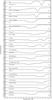 |
Fig. A.1 Transmission of the dust absorption models included in the present analysis for the oxygen region. The oxygen column density has been set here to 1018 cm-2 for all compounds. a) Barrus et al. (1997), b) Parent et al. (2002), c) van Aken et al. (1998), d) Lee et al. (2008). See also Pinto et al. (2010) for details. |
All Tables
All Figures
|
Fig. 1 Upper panel: comparison of the second and first order for RGS1. Lower panel: the ratio of the second to the first order provides an indication of pile up in the spectrum. |
| In the text | |
|
Fig. 2 Light curve of EPIC-pn data as selected in Sect. 2.1. Note that the displayed count rate cannot be used to recover the flux of the source. The bin time is 500 s. |
| In the text | |
|
Fig. 3 Upper panel: residuals to a simple absorbed power law for EPIC-pn and INTEGRAL data. JEMX data have been highlighted for clarity. Lower panel: residuals to the best fit consisting of a black body plus Comptonized emission, modified by both a neutral and ionized absorbing material. EPIC-pn data have been rebinned for display purposes. |
| In the text | |
|
Fig. 4 Upper panel: the best-fit model consists of a black body (dashed line) plus Comptonized emission (dot-dashed line), modified by both a neutral and ionized absorbing material (Table 2). Lower panel: best-fit model superimposed on the EPIC-pn, JEMX and ISGRI spectra. |
| In the text | |
|
Fig. 5 Line equivalent width as a function of the ionic column density for O i, N i and O ii. The velocity dispersions are σv = 10, 100, 200 km s-1. Curves of different ions have been shifted for clarity. |
| In the text | |
|
Fig. 6 Fits in the oxygen region. Here only RGS1 of the most recent observation is displayed for clarity. Upper panel: comparison between a fit only in terms of gas (solid line) and the best fit obtained using dust (dashed line). For comparison an unacceptable fit using olivine (dashed-dotted line) is also displayed. Lower panel: comparison between a fit only in terms of gas (solid line) and the best fit obtained with a mixture of gas and dust (dashed line). See more details in the text. |
| In the text | |
|
Fig. 7 Best fit transmission spectrum (Table 4, Col. (3)) in the oxygen edge region. This allows to compare absorption at different epochs, removing the contribution of the continuum. The upper curves display the transmission of the various absorbing components. Note that for clarity only absorption by oxygen is displayed (i.e. no hydrogen absorption). Data have been rebinned for clarity. |
| In the text | |
|
Fig. 8 Detail of the iron L edge region. Here for clarity we display only the MEG and a displaced RGS2 data set. The best fit (solid line, see Table 5) is compared with pure gas fit with solar abundances (dotted line) and with a mixture of gas and iron-rich olivine (thick solid light line). |
| In the text | |
|
Fig. 9 Best-fit transmission spectrum of the region around the iron LII and LIII edges. This allows us to compare absorption at different epochs, removing the contribution of the continuum. The upper curves display the transmission of the various absorbing components. |
| In the text | |
|
Fig. A.1 Transmission of the dust absorption models included in the present analysis for the oxygen region. The oxygen column density has been set here to 1018 cm-2 for all compounds. a) Barrus et al. (1997), b) Parent et al. (2002), c) van Aken et al. (1998), d) Lee et al. (2008). See also Pinto et al. (2010) for details. |
| In the text | |
Current usage metrics show cumulative count of Article Views (full-text article views including HTML views, PDF and ePub downloads, according to the available data) and Abstracts Views on Vision4Press platform.
Data correspond to usage on the plateform after 2015. The current usage metrics is available 48-96 hours after online publication and is updated daily on week days.
Initial download of the metrics may take a while.