| Issue |
A&A
Volume 539, March 2012
|
|
|---|---|---|
| Article Number | A132 | |
| Number of page(s) | 12 | |
| Section | Interstellar and circumstellar matter | |
| DOI | https://doi.org/10.1051/0004-6361/201117627 | |
| Published online | 06 March 2012 | |
A study of deuterated water in the low-mass protostar IRAS 16293-2422⋆
1
Université de Toulouse, UPS-OMP, IRAP,
Toulouse
France
e-mail: This email address is being protected from spambots. You need JavaScript enabled to view it.
2
CNRS, IRAP, 9
Av. Colonel Roche, BP
44346, 31028
Toulouse Cedex 4,
France
3
Institut de Planétologie et d’Astrophysique de Grenoble (IPAG),
UMR 5274, UJF-Grenoble 1/CNRS, 38041
Grenoble,
France
4
Laboratoire Interdisciplinaire Carnot de Bourgogne, UMR 5209-CNRS,
9 Av. Alain Savary,
BP 47870, 21078
Dijon Cedex,
France
Received:
4
July
2011
Accepted:
6
January
2012
Abstract
Context. Water is a primordial species in the emergence of life, and comets may have brought a large fraction to Earth to form the oceans. To understand the evolution of water from the first stages of star formation to the formation of planets and comets, the HDO/H2O ratio is a powerful diagnostic.
Aims. Our aim is to determine precisely the abundance distribution of HDO towards the low-mass protostar IRAS 16293-2422 and learn more about the water formation mechanisms by determining the HDO/H2O abundance ratio.
Methods. A spectral survey of the source IRAS 16293-2422 was carried out in the framework of the CHESS (Chemical Herschel Surveys of Star forming regions) Herschel key program with the HIFI (Heterodyne Instrument for the Far-Infrared) instrument, allowing detection of numerous HDO lines. Other transitions have been observed previously with ground-based telescopes. The spherical Monte Carlo radiative transfer code RATRAN was used to reproduce the observed line profiles of HDO by assuming an abundance jump. To determine the H2O abundance throughout the envelope, a similar study was made of the H218O observed lines, as the H2O main isotope lines are contaminated by the outflows.
Results. It is the first time that so many HDO and H218O transitions have been detected towards the same source with high spectral resolution. We derive an inner HDO abundance (T ≥ 100 K) of about 1.7 × 10⁻⁷ and an outer HDO abundance (T < 100 K) of about 8 × 10-11. To reproduce the HDO absorption lines observed at 894 and 465 GHz, it is necessary to add an absorbing layer in front of the envelope. It may correspond to a water-rich layer created by the photodesorption of the ices at the edges of the molecular cloud. At a 3σ uncertainty, the HDO/H2O ratio is 1.4–5.8% in the hot corino, whereas it is 0.2–2.2% in the outer envelope. It is estimated at ~4.8% in the added absorbing layer.
Conclusions. Although it is clearly higher than the cosmic D/H abundance, the HDO/H2O ratio remains lower than the D/H ratio derived for other deuterated molecules observed in the same source. The similarity of the ratios derived in the hot corino and in the added absorbing layer suggests that water formed before the gravitational collapse of the protostar, contrary to formaldehyde and methanol, which formed later once the CO molecules had depleted on the grains.
Key words: astrochemistry / ISM: individual objects: IRAS 16293-2422 / ISM: molecules / ISM: abundances
Based on Herschel/HIFI observations. Herschel is an ESA space observatory with science instruments provided by European-led Principal Investigator consortia and with important participation from NASA.
© ESO, 2012
1. Introduction
Water is one of the most important molecules in the solar system and beyond, but an unresolved question remains of how water has evolved from cold prestellar cores to protoplanetary disks and consequently oceans for the Earth’s specific, but probably not isolated, case. In addition to being a primordial ingredient in the emergence of life, this molecule plays an essential role in the process of star formation through the cooling of warm gas. It also controls the chemistry for many species, either in the gas phase or on the grain surfaces. In cold dense cores, the gas-phase water abundance is low, less than about 10-8 (see for example Bergin & Snell 2002; Caselli et al. 2010), while it can reach much higher values in the outflowing gas of the low-mass protostars environments (~10-5–10-4; Liseau et al. 1996; Lefloch et al. 2010; Kristensen et al. 2010) before the solar-type protoplanetary systems are formed.
In standard gas-phase chemistry, H2O forms through ion-molecule reactions that leads to H3O+, which can dissociatively recombine to form H2O (e.g., Bates 1986; Rodgers & Charnley 2002), or through the highly endothermic reaction O + H2 → OH + H, followed by the reaction of OH with H2 (Wagner & Graff 1987; Hollenbach & McKee 1989; Atkinson et al. 2004). The former process is typical of diffuse cloud conditions, whereas the latter only works in regions with high temperatures, such as shocks or hot cores. It has been realized for around 30 years that, in cold and dense regions, H2O is formed much more efficiently on the grains through a series of reactions involving O and H accreted from the gas (e.g., Tielens & Hagen 1982; Jones & Williams 1984; Mokrane et al. 2009; Dulieu et al. 2010; Cuppen et al. 2010). Near protostars, the grain temperature rises above ~100 K, leading to a fast H2O ice desorption (Ceccarelli et al. 1996; Fraser et al. 2001) that increases the H2O gas-phase abundance in the inner part of the envelope called hot core/corino for a high-mass/low-mass protostar (Melnick et al. 2000; Ceccarelli et al. 1999, 2000a).
Deuterated water is likely to form with a similar chemistry to that of water. Theoretically, the HDO/H2O ratio should be high if water has been formed at low temperature, i.e. on cold grain surfaces, and low if it is a product of the photodissociation region or shock chemistry. Indeed, this is caused by the zero-point energy difference in the vibrational potential (Solomon & Woolf 1973). As the deuterated species have higher reduced mass than their undeuterated counterparts, the zero-point energy of the deuterated species is lower (the difference in energy between H2O and HDO is 886 K; Hewitt et al. 2005). Consequently, the enrichment of deuterated water with respect to its main isotopologue takes place at low temperature. The deuteration fraction observed in high-mass hot cores is typically HDO/H2O ≤ 10-3 (Jacq et al. 1990; Gensheimer et al. 1996; Helmich et al. 1996), although higher values (~10-2) have recently been found for Orion (Persson et al. 2007; Bergin et al. 2010). This ratio has also been estimated in the inner envelope of low-mass protostars such as IRAS 16293-2422 (Parise et al. 2005) at about 3%, NGC 1333-IRAS4B (Jørgensen & van Dishoeck 2010) with an upper limit of 0.06%, and NGC 1333-IRAS2A (Liu et al. 2011) with a lower limit of 1%. Deuterated water has also been sought in ices towards several protostars, and has allowed Dartois et al. (2003) and Parise et al. (2003) to obtain upper limits of solid HDO/H2O from 0.5% to 2%.
It is important to know the HDO/H2O ratio throughout the protostar envelope in order to determine how this ratio is preserved after the dispersion of the envelope, when a protoplanetary disk is left over, from which asteroids, comets, and planets may form. Obviously, this ratio is needed in order to evaluate the contribution of comets for transferring water in Earth’s oceans (Morbidelli et al. 2000; Raymond et al. 2004; Villanueva et al. 2009), directly associated with the emergence of life. It seems therefore crucial to determine how similar the observed HDO/H2O ratios in protostellar environments are to those observed in comets and in ocean water on Earth (~0.02%, e.g., Bockelée-Morvan et al. 1998; Lecuyer et al. 1998). Recently, Hartogh et al. (2011) have reported a D/H ratio in the Jupiter family comet 103P/Hartley2, originating in the Kuiper belt, of 0.016, suggesting that some of Earth’s water comes from the same comet family.
IRAS 16293-2422 (hereafter IRAS 16293) is a solar-type protostar situated in the LDN 1689N cloud in Ophiuchus at a distance of 120 pc (Knude & Hog 1998; Loinard et al. 2008). It is constituted of two cores IRAS 16293A and IRAS 16293B separated by ~5″, and the source IRAS 16293A itself could be a binary system (Wootten 1989). Several outflows have also been detected in this source (Castets et al. 2001; Stark et al. 2004; Chandler et al. 2005; Yeh et al. 2008). This Class 0 protostar is the first source where a hot corino has been discovered (Ceccarelli et al. 2000b; Cazaux et al. 2003; Bottinelli et al. 2004). It is also a well-studied case thanks to its high deuterium fractionation. For example, the abundance of doubly deuterated formaldehyde has been estimated between 3 and 16% of the main isotopologue abundance (Ceccarelli et al. 1998, 2001). Methanol also shows a high deuterium fractionation: about 30 ± 20% for CH2DOH, 6 ± 5% for CHD2OH, and ~1.4% for CD3OH (Parise et al. 2004). More recently, Demyk et al. (2010) have determined a methyl formate deuterium fractionation of ~15%, and Bacmann et al. (2010) have concluded that there is a ND/NH ratio between 30% and 100%. Singly deuterated water in IRAS 16293 has been studied with ground-based telescopes by Stark et al. (2004) and Parise et al. (2005). The former find a constant abundance of 3 × 10⁻¹⁰ throughout the envelope with the JCMT observation of the HDO 10,1−00,0 fundamental line at 465 GHz alone, whereas the latter obtain an inner abundance (where T ≥ 100 K) Xin = 1 × 10⁻⁷ and an outer abundance Xout ≤ 1 × 10⁻⁹ using four transitions observed with the IRAM1-30 m telescope, as well as a JCMT2 observation at 465 GHz. Using the water abundances determined from ISO/LWS3 observations, which suffer from both a high beam-dilution and very low spectral resolution (Ceccarelli et al. 2000a), Parise et al. (2005) estimated a deuteration ratio HDO/H2O of about 3% in the hot corino and lower than 0.2% in the outer envelope. Thanks to the spectral survey carried out with Herschel/HIFI towards IRAS 16293 in the framework of the CHESS key program (Ceccarelli et al. 2010), numerous HDO and H2O transitions have been observed at high spectral resolution, allowing an accurate determination of the HDO/H2O ratio in this source. Heavy water (D2O) has also been detected in IRAS 16293 with the 11,1−00,0 fundamental ortho transition at 607 GHz with Herschel/HIFI (Vastel et al. 2010) and the 11,0−10,1 fundamental para transition at 317 GHz with JCMT (Butner et al. 2007). From both transitions, Vastel et al. (2010) estimated a D2O abundance of about 2 × 10-11 in the colder envelope.
The main goal of this paper is to determine the abundance of HDO throughout the protostar envelope, using new HDO collisional coefficients with H2 computed by Faure et al. (2012) and Wiesenfeld et al. (2011), and combining the Herschel/HIFI, JCMT and IRAM data in this source. In Sect. 2, we present the observations and in Sect. 3, the modeling of the HDO and H2O emission distribution in the source using the radiative transfer code RATRAN (Hogerheijde & van der Tak 2000). In Sect. 4, we discuss the derived water deuterium fractionation, and conclude in Sect. 5.
2. Observations
In total, thirteen HDO transitions have been detected towards the solar-type protostar
IRAS 16293, nine with the Herschel HIFI instrument, three with the
IRAM-30 m, and one with the JCMT. Three other transitions observed with HIFI, although not
detected, have been used to derive upper limits. In addition, fifteen transitions of
H2O have been observed
with HIFI. The ortho-H2O
11,0−10,1 fundamental line is
clearly detected, four other transitions are tentatively detected, and ten others were not
detected but their upper limits give constraints on the water abundance. Numerous
 O lines have
been detected but not used since contaminated by the outflows. The
ortho-
O lines have
been detected but not used since contaminated by the outflows. The
ortho- O
11,0−10,1 fundamental line has
also been detected.
O
11,0−10,1 fundamental line has
also been detected.
2.1. HIFI data
In the framework of the guaranteed time key program CHESS (Ceccarelli et al. 2010), we observed the low-mass protostar IRAS 16293
with the HIFI instrument (de Graauw et al. 2010)
onboard the Herschel Space Observatory (Pilbratt et al. 2010). A full spectral coverage was performed in the frequency
ranges [480–1142 GHz] (HIFI bands 1 to 5), [1481–1510 GHz] (HIFI band 6a), and
[1573–1798 GHz] (HIFI bands 6b and 7a). The observations were obtained in March 2010 and
February 2011, using the HIFI Spectral Scan Double Beam Switch (DBS) fast-chop mode with
optimization of the continuum. Twelve HDO lines and fifteen
H2O lines have
been observed in these bands. Table 1 lists, for
all transitions, the observed parameters. The HIFI Wide Band Spectrometer (WBS) was used,
providing a spectral resolution of 1.1 MHz (0.69 km s-1 at 490 GHz and
0.18 km s-1 at 1800 GHz) over an instantaneous bandwidth of 4 × 1 GHz. The
targeted coordinates were
α2000 = 16h32m22 75,
δ2000 = −24°28′34.2″, a position at equal distance of
IRAS 16293 A and B, to measure the emission of both components. The DBS reference
positions were situated approximately 3′ east and west of the source. The forward
efficiency is about 0.96 at all frequencies. The main beam efficiencies used are shown in
Table 1 and are the recommended values from Roelfsema et al. (2012).
75,
δ2000 = −24°28′34.2″, a position at equal distance of
IRAS 16293 A and B, to measure the emission of both components. The DBS reference
positions were situated approximately 3′ east and west of the source. The forward
efficiency is about 0.96 at all frequencies. The main beam efficiencies used are shown in
Table 1 and are the recommended values from Roelfsema et al. (2012).
The data were processed using the standard HIFI pipeline up to frequency and amplitude calibrations (level 2) with the ESA-supported package HIPE 5.1 (Ott 2010) for all the bands except band 3a, processed with the package HIPE 5.2. In the selected observing mode, all lines were observed at least four times (if they are on a receiver band edge), but generally eight times (four in LSB and four in USB) for each polarization. To produce the final spectra, all observations were exported to the GILDAS/CLASS4 software. Using this package, the H and V polarizations at the line frequencies were averaged, weighting them by the observed noise for each spectra. We verified, for all spectra, that no emission from other species was present in the image band. HIFI operates as a double sideband (DSB) receiver, and the gains for the upper and lower sidebands are not necessarily equal. From the in-orbit performances of the instrument (Roelfsema et al. 2012), a sideband ratio of unity is assumed for the HDO transition seen in absorption against the continuum (band 3b). The observed continuum is therefore divided by two to obtain the SSB (single sideband) continuum. The relative calibration budget error of the HIFI instrument is presented in Table 7 of Roelfsema et al. (2012). Considering all the upper limits and estimated errors, we assumed an overall calibration uncertainty of 15% for each line.
2.2. IRAM data
The IRAS 16293 Millimeter And Submillimeter Spectral Survey (TIMASSS; Caux et al. 2011) was performed between 2004 and 2007
at the IRAM-30 m telescope in the frequency range 80–280 GHz and at the JCMT-15 m
telescope in the frequency range 328–368 GHz. The observations were centered on the
IRAS 16293 B source at
α2000 = 16h32m226,
δ2000 = −24°28′33″. In this survey, four HDO lines were
detected, but only three of them (80.578, 225.897, and 241.561 GHz) have been used in this
paper, as the fourth transition at 266.161 GHz lies in a part of the survey where the
calibration uncertainty is very high (Caux et al.
2011). The spectral resolution is 0.31 MHz (~1.2 km s-1) at 81 GHz
and 1 MHz (~1.3 km s-1) at 226 GHz and 242 GHz.
2.3. JCMT data
The HDO 10,1−00,0 fundamental
transition at 464.924 GHz was previously observed by Stark
et al. (2004) on the IRAS 16293 A source
(α2000 = 16h32m2285,
δ2000 = −24°28′35.5″) and by Parise et al. (2005) on the IRAS 16293 B source. The JCMT beam at this
frequency is about 11″. Despite the different pointings, the profiles and the intensities
of the line obtained are similar. This line shows both a wide emission and a narrow deep
absorption (see Fig. 3). The observations are not
optimized for an accurate continuum determination. However, the continuum level is a
crucial parameter in the following modeling. We see thereafter that we can estimate it at
about 1 K thanks to the modeling and the dust emissivity model we chose. It consequently
means that the narrow self-absorption completely absorbs the continuum.
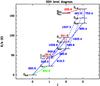 |
Fig. 1 Energy level diagram of the HDO lines. In red, IRAM-30 m observations; in green, JCMT observation; in blue, HIFI observations. The solid arrows show the detected transitions and the dashed arrows the undetected transitions. The frequencies are written in GHz. |
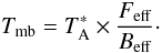
The antenna temperatures of the observations were converted to the
Tmb scale, using the values of the main beam
(Beff) and forward efficiencies
(Feff) given in Table 1 with the usual relation:
 (1)Table 1 and the energy level diagram in Fig. 1 summarize the HDO,
 O and
O transitions
observed towards IRAS 16293 with their flux or upper limit. The 3σ upper
limits on the integrated line intensity are derived following the relation
O and
O transitions
observed towards IRAS 16293 with their flux or upper limit. The 3σ upper
limits on the integrated line intensity are derived following the relation
 (2)with
rms (root mean square) in K, dv, the channel width, in km s-1
and FWHM (full width at half maximum) in km s-1. We assume
FWHM = 5 km s-1, which is the average emission linewidth.
The FWHM given in Table 1 was determined with the
CASSIS5 software by fitting the detected lines
with a Gaussian.
(2)with
rms (root mean square) in K, dv, the channel width, in km s-1
and FWHM (full width at half maximum) in km s-1. We assume
FWHM = 5 km s-1, which is the average emission linewidth.
The FWHM given in Table 1 was determined with the
CASSIS5 software by fitting the detected lines
with a Gaussian.
Using the available spectroscopic databases JPL (Pickett et al. 1998) and CDMS (Müller et al. 2001, 2005), we carefully checked that none of our lines are contaminated by other species.
3. Modeling and results
3.1. Modeling
The spherical Monte Carlo 1D radiative transfer code RATRAN (Hogerheijde & van der Tak 2000), which takes radiative pumping
by continuum emission from dust into account, has been employed to compute the intensity
of the molecular lines and the dust continuum. An input model describing the molecular
H2 density, gas temperature, and velocity field profiles is required, in
order to define the spherical region into many radial cells. The code applies a Monte
Carlo method to iteratively converge on the mean radiation field,
Jν. Level populations of HDO,
O,
O, and
HD18O can then be calculated, once
Jν is determined for every cell. These
level populations are required to map the emission distribution throughout the cloud.
The source structure used in the modeling was determined by Crimier et al. (2010) with a radius extending from 22 AU to 6100 AU
(see Fig. 2); however, the structure in the hot
corino region (T ≥ 100 K) may be uncertain since disks probably exist in
the inner part of the protostellar envelopes. Nevertheless, since the disk characteristics
are unknown, we keep the structure as it is. The radial velocity
 (where M is the stellar mass, G the gravitational
constant and r the radius) is calculated for a stellar mass of
1 M⊙. For a higher mass
(~2 M⊙), the line widths become too broad to reproduce
the line profiles. Moreover, the value of 1 M⊙ agrees with
the mass of the core A, while the mass of the core B is at most about
0.1 M⊙ (Ceccarelli et al.
2000a; Bottinelli et al. 2004; Caux et al. 2011). For a radius greater than 1280 AU,
the envelope is considered as static (the velocity is fixed at 0). This radius corresponds
to a change in the slope of the density profile, marking the transition of the
collapsing/static envelope (Shu 1977), and its
value has been determined by Crimier et al. (2010).
To reproduce the widths of the absorption lines, the turbulence Doppler b-parameter (equal
to 0.6 × FWHM) is fixed at 0.3 km s-1. If a lower
(respectively higher) value is adopted, the modeled absorption lines become too narrow
(respectively too broad) compared with the observations. As source A is more massive than
source B, we considered that the structure is centered on core A. According to
interferometric data of the HDO
31,2−22,1 line at 226 GHz,
deuterated water is mainly emitted by core A (Jørgensen
et al. 2011). Therefore, the assumption of a 1D modeling centered on source A
seems quite reasonable. Because the IRAM observations were pointed on the
IRAS 16293 B source and not on core A and the beam is quite small (~11″) at 226 and
242 GHz, we carefully convolved the resulting map with the telescope beam profile centered
on core B to get the model spectra.
(where M is the stellar mass, G the gravitational
constant and r the radius) is calculated for a stellar mass of
1 M⊙. For a higher mass
(~2 M⊙), the line widths become too broad to reproduce
the line profiles. Moreover, the value of 1 M⊙ agrees with
the mass of the core A, while the mass of the core B is at most about
0.1 M⊙ (Ceccarelli et al.
2000a; Bottinelli et al. 2004; Caux et al. 2011). For a radius greater than 1280 AU,
the envelope is considered as static (the velocity is fixed at 0). This radius corresponds
to a change in the slope of the density profile, marking the transition of the
collapsing/static envelope (Shu 1977), and its
value has been determined by Crimier et al. (2010).
To reproduce the widths of the absorption lines, the turbulence Doppler b-parameter (equal
to 0.6 × FWHM) is fixed at 0.3 km s-1. If a lower
(respectively higher) value is adopted, the modeled absorption lines become too narrow
(respectively too broad) compared with the observations. As source A is more massive than
source B, we considered that the structure is centered on core A. According to
interferometric data of the HDO
31,2−22,1 line at 226 GHz,
deuterated water is mainly emitted by core A (Jørgensen
et al. 2011). Therefore, the assumption of a 1D modeling centered on source A
seems quite reasonable. Because the IRAM observations were pointed on the
IRAS 16293 B source and not on core A and the beam is quite small (~11″) at 226 and
242 GHz, we carefully convolved the resulting map with the telescope beam profile centered
on core B to get the model spectra.
To fit the continuum observed with HIFI from band 1 to band 4, the dust opacity as
function of the frequency has to be constrained by a power-law emissivity model:
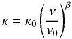 (3)with
β = 1.8,
κ0 = 15 cm2/gdust, and
ν0 = 1012 Hz, which has been used as input in the
RATRAN modeling. Using this emissivity model and the source structure described above, the
continuum of the HDO 10,1−00,0
fundamental line at 465 GHz is predicted at ~1 K. The continuum determination at this
frequency is essential for the modeling because this line shows a deep and narrow
self-absorption. The modeled continuum is shown in Figs. 3 and 4 for the two HDO absorption lines,
whereas it has been subtracted for all the lines that only present emission. The profiles
obtained are resampled at the spectral resolution of the observations. Smoothing was
applied on some observations when the line is undetected or weakly detected (see
Figs. 4 and 10). For the determination of the best-fit parameters by
χ2 minimization (see Sect. 3.3), the spectra are also
resampled to a same spectral resolution for all the lines (0.7 km s-1 for HDO
and 0.6 km s-1 for O,
O, and
HD18O, which correspond to the lowest spectral resolution of the HIFI data).
(3)with
β = 1.8,
κ0 = 15 cm2/gdust, and
ν0 = 1012 Hz, which has been used as input in the
RATRAN modeling. Using this emissivity model and the source structure described above, the
continuum of the HDO 10,1−00,0
fundamental line at 465 GHz is predicted at ~1 K. The continuum determination at this
frequency is essential for the modeling because this line shows a deep and narrow
self-absorption. The modeled continuum is shown in Figs. 3 and 4 for the two HDO absorption lines,
whereas it has been subtracted for all the lines that only present emission. The profiles
obtained are resampled at the spectral resolution of the observations. Smoothing was
applied on some observations when the line is undetected or weakly detected (see
Figs. 4 and 10). For the determination of the best-fit parameters by
χ2 minimization (see Sect. 3.3), the spectra are also
resampled to a same spectral resolution for all the lines (0.7 km s-1 for HDO
and 0.6 km s-1 for O,
O, and
HD18O, which correspond to the lowest spectral resolution of the HIFI data).
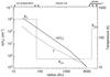 |
Fig. 2 H2 density (solid line) and gas temperature (dashed line) structure of IRAS 16293 determined by Crimier et al. (2010). The expected abundance profile of water is added (dashed-dotted line) on an arbitrary Y-scale. In the colder envelope (T < 100 K), the water molecules are trapped on the grain mantles, whereas in the inner part of the envelope, they are released in gas phase by thermal heating, leading to an enhancement of the abundance. In the outer part of the molecular cloud (AV ~ 1–4), the water abundance can also increase by photodesorption mechanisms. A freeze-out timescale much longer than the protostellar lifetime can also lead to an enhanced abundance when the density is low (~104 cm-3). |
Previous studies (e.g. van Kempen et al. 2008)
have shown that in protostellar envelopes, the dust can become optically thick, preventing
water emission from deep in the envelope to escape. The dust continuum could therefore
hide the higher frequencies HDO and O lines
coming from the hot corino, depending on the source structure and the dust emissivity
model chosen. In fact, we notice here that the dust optical depth is always lower than 1
for all the frequencies lower than 1500 GHz. For the transitions quoted in Table 1 with frequencies higher than 1500 GHz, the dust
opacity only exceeds 1 for temperatures well over 100 K. Consequently, in the case of
IRAS 16293, the dust opacity should not hide the higher frequencies HDO and
O lines as
the dust opacity only becomes thick in the very deep part of the inner envelope.
3.2. HDO collisional rate coefficients
The HDO collisional rates used in this study have recently been computed by Faure et al. (2012) for para-H2(J2 = 0,2) and ortho-H2 (J2 = 1) in the temperature range 5 − 300 K, and for all the transitions with an upper energy level less than 444 K. The methodology used by Faure et al. (2012) is described in detail in Scribano et al. (2010) and Wiesenfeld et al. (2011). These authors present detailed comparisons between the three water-hydrogen isotopologues H2O-H2, HDO-H2, and D2O-H2. Significant differences were observed in the cross sections and rates and were attributed to symmetry, kinematics, and intramolecular (monomer) geometry effects. Moreover, in the case of HDO, rate coefficients with H2 were found to be significantly larger, by up to three orders of magnitude, than the (scaled) H2O-He rate coefficients of Green (1989), which are currently employed in astronomical models (see Fig. 2 of Faure et al. 2012). A significant impact of the new HDO rate coefficients is thus expected in the determination of interstellar HDO abundances, as examined in Sect. 3.3. In the following, we assume that the ortho-to-para ratio of H2 is at local thermodynamic equilibrium (LTE) in each cell of the envelope. The collisional rates for para-H2 were also summed and averaged by assuming a thermal distribution of J2 = 0,2.
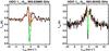 |
Fig. 3 In black: HDO 11,1−00,0 and 11,0−00,0 absorption lines observed at 894 GHz with HIFI and at 465 GHz with JCMT, respectively. In red: HDO modeling without adding the absorbing layer. In green: HDO modeling when adding an absorbing layer with a HDO column density of ~2.3 × 1013 cm-2. The continuum for both the 894 GHz and 465 GHz lines refers to SSB data. |
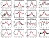 |
Fig. 4 In black: HDO lines observed with HIFI, IRAM, and JCMT. In red: best-fit model obtained when adding an absorbing layer with an HDO column density of ~2.3 × 1013 cm-2 to the structure (see details in text). The best-fit inner abundance is 1.7 × 10⁻⁷ and the best-fit outer abundance is 8 × 10-11. The continuum shown for both the 894 GHz and 465 GHz lines, refers to SSB data. |
3.3. Determination of the HDO abundance
In a first step, we ran a grid of models with one abundance jump at 100 K, in the
so-called hot corino (Ceccarelli et al. 1996, 2000b). The abundance of water is expected to be higher
in the hot corino than in the colder envelope, since the water molecules contained in the
icy grain mantles are released in gas phase, when the temperature is higher than the
sublimation temperature of water, ~100 K (Fraser et al.
2001). Thereafter, the inner abundance (T ≥ 100 K) will be
designated by Xin and the outer abundance (T
< 100 K) by Xout. Both are free
parameters and their best-fit values are determined by a χ2
minimization. To take the line profile into account, the χ2 is
computed from the observed and modeled spectra resampled at a same spectral resolution
(0.7 km s-1 for HDO and 0.6 km s-1 for
O) according
to the following formalism: 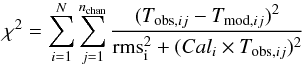 (4)with
N the number of lines i,
nchan the number of channels j for each
line, Tobs,ij and
Tmod,ij the intensity observed and
predicted by the model respectively in channel j of the
line i, rmsi the rms at the
0.7 km s-1 (or 0.6 km s-1) spectral resolution (given in Table 1),
and Cali the calibration
uncertainty. We assumed an overall calibration uncertainty of 15% for each detected line.
(4)with
N the number of lines i,
nchan the number of channels j for each
line, Tobs,ij and
Tmod,ij the intensity observed and
predicted by the model respectively in channel j of the
line i, rmsi the rms at the
0.7 km s-1 (or 0.6 km s-1) spectral resolution (given in Table 1),
and Cali the calibration
uncertainty. We assumed an overall calibration uncertainty of 15% for each detected line.
The best-fit result for this grid of models gives an inner abundance Xin = 1.9 × 10⁻⁷ and an outer abundance Xout = 5 × 10-11 with a reduced χ2 of 3.2. However this model (as well as the other models of this grid) predicts absorption lines that are weaker than observed (see Fig. 3). To correctly reproduce the depth of the absorption in the 465 and 894 GHz lines, while not introducing extra emission in the remaining ones, it is necessary to add an absorbing layer in front of the IRAS 16293 envelope. We notice that the results mainly depend on the HDO column density of the layer, and they are insensitive to the density (for densities lower than ~105 cm-3) and to the temperature (for temperatures lower than ~30 K). The HDO column density of the layer must be about 2.3 × 1013 cm-2. To understand from where the HDO absorptions arise, we can consider two different options.
-
First, the source structure should be extended to a higher outerradius to include the whole molecular cloud. If the absorbinglayer comes from the surrounding gas of the molecular cloudharboring IRAS 16293 and if we assume that theHDO abundance remains constant as in the outer envelope, thiswould imply a surrounding H2 column density of about 2.9 × 1023 cm-2. But this value is considerably too high for a molecular cloud. The N(H2) column density of the ρ Oph cloud has been estimated at ~1.5 × 1022 cm-2 by van Dishoeck et al. (1995) and at ≳5 × 1022 cm-2 by Caux et al. (1999). Adding a molecular cloud with these characteristics to the structure determined by Crimier et al. (2010) does not allow deep absorption lines to be modeled. This hypothesis is therefore insufficient to explain the deep HDO absorption lines.
-
Consequently, the only way to explain the absorption lines consists in assuming a drop abundance structure. Such a structure in the low-mass protostars has already been inferred for several molecules like CO and H2CO (Schöier et al. 2004; Jørgensen et al. 2004, 2005). The raising of the abundance in the outermost regions of the envelope is explained by a longer depletion timescale than the lifetime of the protostars (~104−105 years) for H2 densities lower than ~104−105 cm-3 (e.g., Caselli et al. 1999; Jørgensen et al. 2004). On the other hand, Hollenbach et al. (2009) have shown that, at the edge of molecular clouds, the icy mantles are photodesorbed by the UV photons, giving rise to an extended layer with a higher water abundance for a visual extinction AV ~ 1–4 mag (for G0 = 1). Assuming an AV of ~1–4 mag and the relation N(H2)/AV = 9.4 × 1020 cm-2 mag-1 (Frerking et al. 1982), the abundance of HDO in this water-rich layer created by the photodesorption of the ices should be about 6 × 10⁻⁹ − 2.4 × 10⁻⁸. We see thereafter, when analyzing the
O
lines, that this hypothesis is nicely consistent with the theoretical predictions by
Hollenbach et al. (2009). For water, both
effects may play a role.
 |
Fig. 5 χ2 contours at 1σ, 2σ, and 3σ obtained when adding an absorbing layer with a HDO column density of 2.3 × 1013 cm-2 to the structure. The results are obtained with the collisional coefficients with ortho and para-H2 determined by Faure et al. (2012). The best-fit model is represented by the symbol “+”. The reduced χ2 is about 2.4. |
As the absorption of the two fundamental lines is reproduced with this outer component
(see Fig. 3), we ran a second grid of models adding
this absorbing layer. The best-fit is obtained for
Xin = 1.7 × 10⁻⁷ and
Xout = 8 × 10-11 with a
 of 2.4. With
the current parameters, a simultaneous fit of all the HIFI, IRAM, and JCMT data is
presented in Fig. 4. The contours of
χ2 at 1σ, 2σ, and
3σ, which respectively represent a confidence of 68.26%, 95.44%, and
99.73% of enclosing the true values of Xin and
Xout, are shown in Fig. 5, computed with the method of Lampton et al.
(1976). The contours at 1σ, 2σ, and
3σ correspond respectively to
of 2.4. With
the current parameters, a simultaneous fit of all the HIFI, IRAM, and JCMT data is
presented in Fig. 4. The contours of
χ2 at 1σ, 2σ, and
3σ, which respectively represent a confidence of 68.26%, 95.44%, and
99.73% of enclosing the true values of Xin and
Xout, are shown in Fig. 5, computed with the method of Lampton et al.
(1976). The contours at 1σ, 2σ, and
3σ correspond respectively to  +2.3,
+6.17, and
+11.8 when the
number of adjustable parameters is two (here Xin and
Xout). The confidence intervals of
Xin and Xout at
3σ are 1.53 × 10⁻⁷ − 2.21 × 10⁻⁷ and
4.6 × 10⁻¹¹−1.0 × 10⁻¹⁰, respectively.
+2.3,
+6.17, and
+11.8 when the
number of adjustable parameters is two (here Xin and
Xout). The confidence intervals of
Xin and Xout at
3σ are 1.53 × 10⁻⁷ − 2.21 × 10⁻⁷ and
4.6 × 10⁻¹¹−1.0 × 10⁻¹⁰, respectively.
In the hot corino, most of the HDO lines are optically thick, except the 81, 226, 242, and 482 GHz transitions that show an opacity ≲1. Since the emission from most of the HDO lines originates both in the hot corino and the outer envelope, the use of a simple rotational-diagram analysis to estimate the total column density of HDO is not appropriate. Figure 6 represents the normalized populations of some levels (up to 31,2) as a function of the distance from the center of the protostar, computed by RATRAN through the equation of statistical equilibrium. These level populations are then used to determine the emission distribution of deuterated water by using a ray-tracing method. This figure also shows that the absorbing layer is mainly constrained by the ground state transitions as 11,1−00,0, and 10,1−00,0.
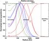 |
Fig. 6 Normalized level populations of HDO computed by RATRAN, as a function of the radius of the protostar envelope. To avoid confusion, the population of levels 20,2, 21,1, and 31,2 are indicated by dashed lines. The HDO 11,1 level population jump visible at ~1300 AU is an artifact due to the change of the velocity field at the interface between the infalling envelope and the static envelope. |
The 81 GHz 11,0−11,1 transition observed at IRAM-30 m is not reproduced well by the best-fit model. The disagreement could be due to a blending effect at this frequency. Nevertheless, it is ruled out for the species included in the JPL and CDMS databases. Calibration could also be questioned at this frequency. But it seems rejected since the profile obtained with the best-fit model differs from the observing profile. Another explanation could come from the assumption of spherical symmetry. Interferometric data of the HDO 31,2−22,1 transition show that, in addition to the main emission coming from the source A, a weaker component of HDO is emitted at about 6″ from core A (see Fig. 20 in Jørgensen et al. 2011). The beam size of the IRAM-30 m telescope at 81 GHz encompasses this component and could explain the lack of predicted flux as well as the different line profile. This hypothesis seems consistent with the lower frequency HIFI lines (491, 509, and 600 GHz) for which the best-fit model misses flux.
The derived abundances for HDO agrees with the 3σ upper limit (0.16 K km s-1) of the HD18O 11,1−00,0 transition observed in our spectra at 883 GHz. Assuming an HD16O/HD18O ratio of 500 (Wilson & Rood 1994), value at the galactocentric distance of IRAS 16293, the modeling predicts an integrated intensity of 0.15 K km s-1.
To obtain consistent profiles of the model compared with the observations, the LSR velocity, VLSR, is about 4.2 km s-1 for the HIFI and JCMT lines, whereas it is about 3.6 km s-1 for the three IRAM lines. This discrepancy of the velocity in the modeling could be explained by the origin of the emission of the lines. The 4.2 km s-1 velocity component could represent the velocity of the envelope. For example, the velocity of the absorption lines of the fundamental transitions of D2O tracing the cold envelope of IRAS 16293 and detected by JCMT (Butner et al. 2007) and by HIFI (Vastel et al. 2010) is 4.15 and 4.33 km s-1, respectively. Even if some HIFI lines trace both the inner part and the outer part of the envelope, the velocity of the outer envelope should dominate because of a smaller line widening in the outer envelope. In contrast, the flux of IRAM lines at 226 and 242 GHz only trace the hot corino (see Figs. 1 and 6). Their velocity (~3.6 km s-1) is lower, in agreement with the velocity of the core A (VLSR ~ 3.9 km s-1).
As previous studies regarding HDO used the collisional coefficients computed by Green (1989), we have run a grid of models with these
rates for a comparison. The simultaneous best-fit of all the transitions using these rates
is obtained for an inner abundance Xin = 2.0 × 10⁻⁷
and an outer abundance Xout = 1 × 10-11. The inner
abundance is similar to what we found above with the collisional coefficients determined
by Faure et al. (2012). However, the outer
abundance is a factor of 8 lower. The χ2 also gives a higher
value ( ), therefore showing that the
observations are better reproduced with rates with H2 than with He.
), therefore showing that the
observations are better reproduced with rates with H2 than with He.
 |
Fig. 7 Comparison of the profiles of the HDO (in black) and
|
3.4. Determination of the water abundance
To determine the H2O abundance throughout the envelope, we used all the
O transitions
in the HIFI range (see Table 1). The only
transition observable in the TIMASSS spectral survey is contaminated by the
CH3OCH3 species at 203.4 GHz. The profiles of the observed
O lines
suggest, by the presence of wings, that the lines are contaminated by the outflows. Unlike
the O lines that
show a width ≳ 10 km s-1, the O line widths
are similar to the HDO lines (see Fig. 7,
~5 km s-1) and no wings are seen in the
O detected
transitions (see Fig. 10). Consequently, the outflow
does not probably contribute to a large extent to the emission of the
O lines.
We used the H2O collisional coefficients determined by Faure et al. (2007) and assumed a
O/O ratio equal
to 500 (Wilson & Rood 1994), as well as a
O ortho/para
ratio of 3. As for HDO, in a first step, we ran a grid of models for different inner and
outer abundances without adding the absorbing layer. The best-fit parameters of the
χ2 minimization are
Xin(O) = 1 ×
10-8 and
Xout(O) = 3 ×
10-11 and the reduced χ2 is about 1.9. The inner
abundance of water is therefore 5 × 10⁻⁶, whereas the outer abundance is 1.5
× 10-8. Figure 8 shows the
χ2 contours at 1σ, 2σ, and
3σ. A calibration uncertainty of 15% has been assumed for the 548 GHz
transition and the tentatively detected ones (1096, 1102, 994, and 745 GHz). At
3σ, the outer abundance of O varies
between 9 × 10-12 and 4.9 × 10⁻¹¹, whereas the inner abundance is in
the interval 7.6 × 10⁻⁹ − 2.1 × 10⁻⁸. Using the best-fit values
found for Xin and Xout, it is
necessary, in order to reproduce the weak absorption of the
11,0−10,1 line at 548 GHz, to
add an absorbing layer with a O column
density of about 1 × 1012 cm-2. For higher column densities, the
models predict absorptions that are too deep for the ortho and para fundamental
transitions (see Fig. 9). For a visual extinction
AV ~ 1–4 mag, the H2O abundance in the
photodesorption layer is 1.3−5.3 × 10⁻⁷. This value is in very good agreement
with the values predicted in photodesorption layers by the model of Hollenbach et al. (2009), about 1.5−3 × 10⁻⁷. The model
predictions with this absorbing layer are shown in Fig. 10. We cannot rule out a remnant contribution of the outflows in view of the
profile of 548 GHz line, but this outflow contribution to the bulk of the emission is very
likely negligible for the other transitions.
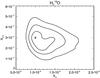 |
Fig. 8 χ2 contours at 1σ,
2σ, and 3σ obtained for
|
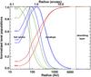 |
Fig. 9 Normalized level populations of |
 |
Fig. 10 In black: |
In the hot corino, among the o-O
transitions, only the 489 and 1181 GHz lines are optically thin, whereas among the
p-O
transitions, only the 970, 1189, and 1606 GHz lines show an opacity lower than 1. The
emission of most of the transitions comes from both the hot corino and the outer envelope
(see Fig. 9). Similarly to HDO, a rotational diagram
analysis therefore cannot be considered for O.
The ortho-O
11,0−10,1 transition at
552 GHz has also been detected. To check the validity of the results, we ran a model
similar to what has been done for O, assuming a
ratio 18O/17O of 4 (Wouterloot
et al. 2008). Figure 11 shows the predicted
models for the 552 GHz line, as well as the para-O 11,1−00,0
fundamental line undetected at 1107 GHz for the best-fit of
O, i.e. for
an inner O abundance
of 2.5 × 10⁻⁹ and an outer O abundance
of 7.5 × 10⁻¹². A prediction with twice the inner abundance, situated in the
3σ contour of O, is also
presented (Fig. 11). We see that the
O predictions
agrees with the O results,
confirming the water abundances derived.
HDO/H2O ratio.
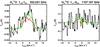 |
Fig. 11 In black: fundamental |
4. Discussion
The study of HDO in the deeply embedded low-mass protostar IRAS 16293 had already been undertaken by Stark et al. (2004), then by Parise et al. (2005), leading to different results. Stark et al. (2004) used a constant [HDO]/[H2] abundance of 3 × 10⁻¹⁰ throughout the envelope to fit the 10,1−00,0 transition at 465 GHz best, resulting in an HDO/H2O ratio in the warm inner envelope of a few times 10-4. However, their best-fit cannot reproduce the deep absorption feature. Also, unlike our study, they do not succeed in reproducing the line width without introducing an outflow contribution; however, the model obtained with the outflow component fails to match simultaneously the line width and the peak intensity. This could be explained by their source structure and the assumption of a constant abundance throughout the envelope. The dust temperature is restricted to a range from 12 K to 115 K. A structure with a lower inner radius (consequently an higher temperature) and an abundance rising in the inner part of the envelope may allow the line to become broader and reproduce the observation. Moreover, the peak intensities predicted by their model for the lines at 226 and 241 GHz (0.001 K and 0.006 K, respectively) are clearly lower than what we observe here (0.30 and 0.32 K, respectively). Afterwards, the results obtained by Stark et al. (2004) have been questioned by the study of Parise et al. (2005). Using IRAM and JCMT observations, they have found an enhancement of the abundance of HDO in the hot corino (Xin ~ 1 × 10⁻⁷) with respect to the outer envelope (Xout ≤ 1 × 10⁻⁹), in agreement with our results using both the collisional coefficients with He by Green (1989) and with ortho and para-H2 by Faure et al. (2012) (see Sect. 3.3). However, their results did not take the line profiles into account, specifically the deep absorption of the ground state transitions, and only allowed a rather high upper limit of the outer abundance to be derived.
Parise et al. (2005) conclude there is a jump in the
HDO/H2O ratio in the inner part of the envelope, using the
H2O abundance determined by Ceccarelli et al.
(2000a). Nevertheless, our results on the water abundance are quite different.
Using O data from
ISO/LWS, highly diluted in a beam width of about 80″, Ceccarelli et al. (2000a) obtained an outer abundance of 5 × 10⁻⁷,
while we found an outer abundance lower than 3.5 × 10⁻⁸. However, their derived
inner abundance of ~3 × 10⁻⁶ is not so very different from our value,
Xin(H2O) ~ 5 × 10⁻⁶. The disagreement
on determining the outer abundance can easily be explained by the fact that Ceccarelli et al. (2000a) used
O data,
contaminated by the outflows that must be added in the modeling. The gas temperature was
computed by assuming the water abundance derived by the ISO observations. However, since the
gas is practically thermally coupled with the dust, the impact in the gas temperature is
certainly negligible. The largest difference between the gas and dust temperature is less
than 10% (Crimier et al. 2010). The discrepancy on
the water abundance therefore results in a different deuteration ratio in the outer
envelope. Considering the 3σ uncertainty, the enhancement of the water
deuterium fractionation in the hot corino cannot be confirmed in our study, in contrast to
what was concluded in Parise et al. (2005).
Table 2 summarizes the HDO/H2O ratio
determined by our analysis in the inner and outer envelope, as well as an estimation of this
ratio in the absorbing layer. With a 3σ uncertainty, the water
fractionation could be similar throughout the cloud with a HDO/H2O ratio between
1.4% and 5.8% in the inner part and between 0.2% and 2.2% in the outer part. Also the
HDO/H2O ratio obtained here is in agreement with the upper limits of solid
HDO/H2O (from 0.5% to 2%) determined by observations of OH and OD stretch bands
in four low-mass protostars (Dartois et al. 2003;
Parise et al. 2003).
A consequential result of this paper is the similarity of the HDO/H2O ratio derived in the hot corino (~1.4–5.8%) and in the added outer absorbing layer (~4.8%). Indeed, the ratio is within the same order of magnitude, although the densities of these two regions are considerably different. The density in the hot corino is a few times 108 cm-3. In the absorbing layer, it is about 103 − 105 cm-3. Consequently, water shows a different behavior from other molecules such as methanol and formaldehyde, that need CO ices to be formed. In particular, Bacmann et al. (2003, 2007) show that the deuteration of H2CO and CH3OH increases with the CO depletion in starless dense cores, increasing itself with the H2 density (Bacmann et al. 2002). The H2CO and CH3OH deuteration is therefore sensitive to the density of the medium in which they form. In contrast, the HDO/H2O ratio does not show any difference for different H2 densities. This would therefore mean that water has formed before the collapse of the protostar and that the HDO/H2O ratio has been preserved during the gravitational collapse. The deuteration fractionation of water would therefore remain similar, both in the inner region of the protostar, where the density has strongly increased, and in the outer region that has not been affected by the collapse. Another argument emphasizes this hypothesis. To obtain such high deuteration ratios of HDCO/H2CO (~15%; Loinard et al. 2001) and CH2DOH/CH3OH (~30%; Parise et al. 2004) in IRAS 16293 compared with HDO/H2O ~ 3%, the density at which the molecules form should be higher for the H2CO and CH3OH formation than for water formation. The collapse should already have started to allow the CO molecules to freeze-out and form formaldehyde and methanol at the grain surface. On the contrary, water would form at low densities in the early stages of the star formation before the protostellar collapse, as suggested by Dartois et al. (2003) and Parise et al. (2003). This is also consistent with the fact that H2O ices appear at relatively low extinction in the direction of the Taurus cloud (e.g. Jones & Williams 1984). Recently, similar conclusions have been mentioned in Cazaux et al. (2011). Using a grain surface chemistry model, they show that the deuteration of formaldehyde is sensitive to the gas D/H ratio as the cloud undergoes gravitational collapse, while the HDO/H2O ratio is constant as the cloud collapses and is set during the formation of ices in the translucent cloud.
The HDO/H2O ratio in the low-mass protostar IRAS 16293 is close to what is found in the low-mass protostar NGC 1333-IRAS2A, as determined by Liu et al. (2011): higher than 1% in the hot corino and between 0.9% and 18% at 3σ. However, this ratio of a few percent does not seem typical of all the Class 0 protostars since an upper limit of 6 × 10⁻⁴ has been determined in the inner part of the envelope of the low-mass protostar NGC 1333-IRAS4B (Jørgensen & van Dishoeck 2010). The determination of the water deuterium fractionation in a larger sample of Class 0 protostars would allow us to know, from a statistical point of view, whether the HDO/H2O ratio is rather about 10-4 − 10-3 as observed in the NGC 1333-IRAS4B protostar, in comets (~3 × 10⁻⁴; e.g. Bockelée-Morvan et al. 1998) and in the Earth’s oceans (~1.5 × 10⁻⁴; Lecuyer et al. 1998) or rather about a few percent, like the young stellar objects NGC 1333-IRAS2A and IRAS 16293. With a value of about 10-4 in the protostellar phase, the fractionation ratio could be conserved throughout the different stages of the star formation until the formation of the the solar-system objects. Higher values in the protostellar phase invoke mechanisms in the gas phase and/or on the grain surfaces to explain the decrease in the deuterium fractionation for water from the protostar formation to the comets and solar system formation. The determination of the HDO/H2O ratio in a larger sample would allow us to understand whether the deuteration of water in protostars is somewhat similar to the solar system value and whether the environment or the conditions for the prestellar core phase play a role.
Finally, we can estimate for the first time the D2O/H2O ratio in a
low-mass protostar. According to the results of Vastel
et al. (2010), the column density of D2O in the cold envelope
(T < 30 K) is
1.65 ± 1.41 × 1012 cm-2 at a 3σ uncertainty. If we
consider that the absorption of the two D2O fundamental lines can be both due to
the cold envelope (T < 30 K), as well as to the
absorbing layer, the D2O/H2O ratio is on average about 10-3
and in the interval 1.1 × 10⁻⁴ − 3.75 × 10⁻³ at 3σ.
As for the D2O/HDO ratio, it is about 6% and between 0.8% and 11.6% at
3σ. The HDO/H2O and D2O/H2O ratio follow
the statistical distribution (even considering the 3σ uncertainty) as
determined in Butner et al. (2007):
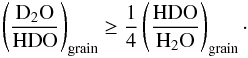 (5)These estimations
of deuteration ratios in a low-mass protostar will certainly provide better constraints on
the gas-grain chemistry models. Indeed, HDO is trapped on the grain surfaces before the
thermal desorption due to the heating from the accreting protostar or before its
photodesorption at the edges of the molecular cloud.
(5)These estimations
of deuteration ratios in a low-mass protostar will certainly provide better constraints on
the gas-grain chemistry models. Indeed, HDO is trapped on the grain surfaces before the
thermal desorption due to the heating from the accreting protostar or before its
photodesorption at the edges of the molecular cloud.
5. Conclusion
This study is the first one to use such a large number of lines to model deuterated water.
Thanks to the numerous HDO transitions observed with Herschel/HIFI and four
other lines observed with ground-based telescopes, we have succeeded in accurately
determining the abundance of HDO throughout the envelope of the protostar and particularly
the outer abundance that Parise et al. (2005) could
not constrain. To estimate the abundances, new collisional coefficients computed with ortho
and para-H2 by Faure et al. (2012) and for
a wide range of temperatures were used. The best-fit inner abundance
Xin(HDO) is about 1.7 × 10⁻⁷, whereas the best-fit
outer abundance Xout(HDO) is about 8 × 10-11. To
model the deep HDO absorption lines, it has been necessary to add an outer absorbing layer
with an HDO column density of 2.3 × 1013 cm-2. In addition, detections
of several O transitions, as
well as small upper limits on other transitions, have allowed us to constrain both the inner
and outer water abundances. Assuming a standard isotopic ratio
O/O = 500, the
inner abundance of water is about 5 × 10⁻⁶ and the outer abundance about
1.5 × 10⁻⁸. The water column density in the added absorbing layer is about
5 × 1014 cm-2. If we consider that this absorbing layer is created
by the photodesorption of the ices at an AV of ~1–4 mag, the
water abundance is about 1.3–5.3 × 10⁻⁷ nicely consistent with the values
predicted by Hollenbach et al. (2009). The deuterium
fractionation of water is therefore about 1.4–5.8% in the hot corino, 0.2–2.2% in the colder
envelope, and 4.8% in the added absorbing layer. The 3σ uncertainties
determined in both the inner and the outer part of the envelope are small due to both the
well constrained HDO and O abundances (see
Table 2). These results do not permit any conclusion on an enhancement of the fractionation
ratio in the inner envelope with respect to the outer envelope. The similar ratios derived
in the hot corino and in the absorbing layer suggest that water forms before the
gravitational collapse of the protostar, unlike formaldehyde and methanol, which form later
after the CO molecules have depleted on the grains. In the cold envelope
(T < 30 K), the D2O/HDO ratio is
estimated with a value of 6%. The HDO/H2O ratios found here are clearly higher
than those observed in comets (~0.02%). The water deuterium fractionation ratio has to be
estimated in more low-mass protostars to determine if IRAS 16293 is an exception among the
Class 0 sources or a typical protostar that could lead to the formation of a planetary
system similar to our Solar System. In the latter case, processes should be at work to
reprocess the water deuteration ratio before the cometary formation stage.
The strong constraints obtained here emphasize the necessity to observe several lines in a
broad frequency and energy range, as done with the HIFI spectral survey, to precisely
estimate the water deuterium fractionation. In particular, the
HDO 11,1−00,0 fundamental line
at 894 GHz is a key line in the modeling because it shows emission both from the hot corino
and the outer part of the envelope. In addition, both this transition and the
10,1−00,0 transition at
465 GHz present a deep absorption probing the absorbing layer. The
HDO 31,2−22,1 and
21,1−21,2 transitions observed
at 226 and 242 GHz, respectively, with the IRAM-30 m telescope also bring useful information
as they entirely probe the hot corino. These transitions, as well as several
O transitions, lie in
the ALMA6 spectral range that will hopefully allow the
HDO/H2O ratio to be studied and constrained in many low-mass protostars with
very high spatial resolution.
Institut de RadioAstronomie Millimétrique.
James Clerk Maxwell Telescope.
Infrared Space Observatory/Long Wavelength Spectrometer.
http://www.iram.fr/IRAMFR/GILDAS/
CASSIS (http://cassis.cesr.fr) has been developed by IRAP-UPS/CNRS.
Atacama Large Millimeter Array.
Acknowledgments
HIFI was designed and built by a consortium of institutes and university departments from across Europe, Canada, and the United States under the leadership of SRON Netherlands Institute for Space Research, Groningen, The Netherlands, with major contributions from Germany, France and the US Consortium members are: Canada: CSA, U. Waterloo; France: CESR, LAB, LERMA, IRAM; Germany: KOSMA, MPIfR, MPS; Ireland, NUI Maynooth; Italy: ASI, IFSI-INAF, Osservatorio Astrofisico di Arcetri-INAF; The Netherlands: SRON, TUD; Poland: CAMK, CBK; Spain: Observatorio Astronómico Nacional (IGN), Centro de Astrobiología (CSIC-INTA). Sweden: Chalmers University of Technology – MC2, RSS & GARD; Onsala Space Observatory; Swedish National Space Board, Stockholm University – Stockholm Observatory; Switzerland: ETH Zurich, FHNW; USA: Caltech, JPL, NHSC. We thank many funding agencies for financial support. L.W. thanks the COST “Chemical Cosmos” program, as well as the CNRS national program “Physique et Chimie du Milieu Interstellaire” for partial support. The collision coefficients calculations presented in this paper were performed at the Service Commun de Calcul Intensif de l’Observatoire de Grenoble (SCCI).
References
- Atkinson, R., Baulch, D. L., Cox, R. A., et al. 2004, Atmos. Chem. Phys., 4, 1461 [NASA ADS] [CrossRef] [Google Scholar]
- Bacmann, A., Lefloch, B., Ceccarelli, C., et al. 2002, A&A, 389, L6 [NASA ADS] [CrossRef] [EDP Sciences] [Google Scholar]
- Bacmann, A., Lefloch, B., Ceccarelli, C., et al. 2003, ApJ, 585, L55 [NASA ADS] [CrossRef] [EDP Sciences] [Google Scholar]
- Bacmann, A., Lefloch, B., Parise, B., Ceccarelli, C., & Steinacker, J. 2007, in Molecules in Space and Laboratory [Google Scholar]
- Bacmann, A., Caux, E., Hily-Blant, P., et al. 2010, A&A, 521, L42 [NASA ADS] [CrossRef] [EDP Sciences] [Google Scholar]
- Bates, D. R. 1986, ApJ, 306, L45 [NASA ADS] [CrossRef] [Google Scholar]
- Bergin, E. A., & Snell, R. L. 2002, ApJ, 581, L105 [NASA ADS] [CrossRef] [Google Scholar]
- Bergin, E. A., Phillips, T. G., Comito, C., et al. 2010, A&A, 521, L20 [NASA ADS] [CrossRef] [EDP Sciences] [Google Scholar]
- Bockelée-Morvan, D., Gautier, D., Lis, D. C., et al. 1998, Icarus, 133, 147 [NASA ADS] [CrossRef] [Google Scholar]
- Bottinelli, S., Ceccarelli, C., Neri, R., et al. 2004, ApJ, 617, L69 [NASA ADS] [CrossRef] [Google Scholar]
- Butner, H. M., Charnley, S. B., Ceccarelli, C., et al. 2007, ApJ, 659, L137 [NASA ADS] [CrossRef] [Google Scholar]
- Caselli, P., Walmsley, C. M., Tafalla, M., Dore, L., & Myers, P. C. 1999, ApJ, 523, L165 [NASA ADS] [CrossRef] [Google Scholar]
- Caselli, P., Keto, E., Pagani, L., et al. 2010, A&A, 521, L29 [NASA ADS] [CrossRef] [EDP Sciences] [Google Scholar]
- Castets, A., Ceccarelli, C., Loinard, L., Caux, E., & Lefloch, B. 2001, A&A, 375, 40 [NASA ADS] [CrossRef] [EDP Sciences] [Google Scholar]
- Caux, E., Ceccarelli, C., Castets, A., et al. 1999, A&A, 347, L1 [NASA ADS] [Google Scholar]
- Caux, E., Kahane, C., Castets, A., et al. 2011, A&A, 532, A23 [NASA ADS] [CrossRef] [EDP Sciences] [Google Scholar]
- Cazaux, S., Tielens, A. G. G. M., Ceccarelli, C., et al. 2003, ApJ, 593, L51 [NASA ADS] [CrossRef] [Google Scholar]
- Cazaux, S., Caselli, P., & Spaans, M. 2011, ApJ, 741, L34 [NASA ADS] [CrossRef] [Google Scholar]
- Ceccarelli, C., Hollenbach, D. J., & Tielens, A. G. G. M. 1996, ApJ, 471, 400 [Google Scholar]
- Ceccarelli, C., Castets, A., Loinard, L., Caux, E., & Tielens, A. G. G. M. 1998, A&A, 338, L43 [NASA ADS] [Google Scholar]
- Ceccarelli, C., Caux, E., Loinard, L., et al. 1999, A&A, 342, L21 [NASA ADS] [Google Scholar]
- Ceccarelli, C., Castets, A., Caux, E., et al. 2000a, A&A, 355, 1129 [NASA ADS] [Google Scholar]
- Ceccarelli, C., Loinard, L., Castets, A., Tielens, A. G. G. M., & Caux, E. 2000b, A&A, 357, L9 [NASA ADS] [Google Scholar]
- Ceccarelli, C., Loinard, L., Castets, A., et al. 2001, A&A, 372, 998 [NASA ADS] [CrossRef] [EDP Sciences] [Google Scholar]
- Ceccarelli, C., Bacmann, A., Boogert, A., et al. 2010, A&A, 521, L22 [NASA ADS] [CrossRef] [EDP Sciences] [Google Scholar]
- Chandler, C. J., Brogan, C. L., Shirley, Y. L., & Loinard, L. 2005, ApJ, 632, 371 [NASA ADS] [CrossRef] [Google Scholar]
- Crimier, N., Ceccarelli, C., Maret, S., et al. 2010, A&A, 519, A65 [NASA ADS] [CrossRef] [EDP Sciences] [Google Scholar]
- Cuppen, H. M., Ioppolo, S., Romanzin, C., & Linnartz, H. 2010, Phys. Chem. Chem. Phys. (Incorporating Faraday Transactions), 12, 12077 [NASA ADS] [CrossRef] [Google Scholar]
- Dartois, E., Thi, W.-F., Geballe, T. R., et al. 2003, A&A, 399, 1009 [NASA ADS] [CrossRef] [EDP Sciences] [Google Scholar]
- de Graauw, T., Helmich, F. P., Phillips, T. G., et al. 2010, A&A, 518, L6 [NASA ADS] [CrossRef] [EDP Sciences] [Google Scholar]
- Demyk, K., Bottinelli, S., Caux, E., et al. 2010, A&A, 517, A17 [NASA ADS] [CrossRef] [EDP Sciences] [Google Scholar]
- Dulieu, F., Amiaud, L., Congiu, E., et al. 2010, A&A, 512, A30 [NASA ADS] [CrossRef] [EDP Sciences] [Google Scholar]
- Faure, A., Crimier, N., Ceccarelli, C., et al. 2007, A&A, 472, 1029 [NASA ADS] [CrossRef] [EDP Sciences] [Google Scholar]
- Faure, A., Wiesenfeld, L., Scribano, Y., & Ceccarelli, C. 2012, MNRAS, 420, 699 [NASA ADS] [CrossRef] [MathSciNet] [Google Scholar]
- Fraser, H. J., Collings, M. P., McCoustra, M. R. S., & Williams, D. A. 2001, MNRAS, 327, 1165 [NASA ADS] [CrossRef] [Google Scholar]
- Frerking, M. A., Langer, W. D., & Wilson, R. W. 1982, ApJ, 262, 590 [NASA ADS] [CrossRef] [Google Scholar]
- Gensheimer, P. D., Mauersberger, R., & Wilson, T. L. 1996, A&A, 314, 281 [NASA ADS] [Google Scholar]
- Green, S. 1989, ApJS, 70, 813 [NASA ADS] [CrossRef] [Google Scholar]
- Hartogh, P., Lis, D. C., Bockelée-Morvan, D., et al. 2011, Nature, 478, 218 [NASA ADS] [CrossRef] [PubMed] [Google Scholar]
- Helmich, F. P., van Dishoeck, E. F., & Jansen, D. J. 1996, A&A, 313, 657 [NASA ADS] [Google Scholar]
- Hewitt, A. J., Doss, N., Zobov, N. F., Polyansky, O. L., & Tennyson, J. 2005, MNRAS, 356, 1123 [NASA ADS] [CrossRef] [Google Scholar]
- Hogerheijde, M. R., & van der Tak, F. F. S. 2000, A&A, 362, 697 [NASA ADS] [Google Scholar]
- Hollenbach, D., & McKee, C. F. 1989, ApJ, 342, 306 [NASA ADS] [CrossRef] [Google Scholar]
- Hollenbach, D., Kaufman, M. J., Bergin, E. A., & Melnick, G. J. 2009, ApJ, 690, 1497 [CrossRef] [Google Scholar]
- Jacq, T., Walmsley, C. M., Henkel, C., et al. 1990, A&A, 228, 447 [NASA ADS] [Google Scholar]
- Jones, A. P., & Williams, D. A. 1984, MNRAS, 209, 955 [NASA ADS] [CrossRef] [Google Scholar]
- Jørgensen, J. K., & van Dishoeck, E. F. 2010, ApJ, 725, L172 [NASA ADS] [CrossRef] [Google Scholar]
- Jørgensen, J. K., Schöier, F. L., & van Dishoeck, E. F. 2004, A&A, 416, 603 [NASA ADS] [CrossRef] [EDP Sciences] [Google Scholar]
- Jørgensen, J. K., Schöier, F. L., & van Dishoeck, E. F. 2005, A&A, 437, 501 [NASA ADS] [CrossRef] [EDP Sciences] [Google Scholar]
- Jørgensen, J. K., Bourke, T. L., Nguyn Lu’O’Ng, Q., & Takakuwa, S. 2011, A&A, 534, A100 [NASA ADS] [CrossRef] [EDP Sciences] [Google Scholar]
- Knude, J., & Hog, E. 1998, A&A, 338, 897 [NASA ADS] [Google Scholar]
- Kristensen, L. E., Visser, R., van Dishoeck, E. F., et al. 2010, A&A, 521, L30 [NASA ADS] [CrossRef] [EDP Sciences] [Google Scholar]
- Lampton, M., Margon, B., & Bowyer, S. 1976, ApJ, 208, 177 [NASA ADS] [CrossRef] [Google Scholar]
- Lecuyer, C., Gillet, P., & Robert, F. 1998, Chem. Geol., 145, 249 [NASA ADS] [CrossRef] [Google Scholar]
- Lefloch, B., Cabrit, S., Codella, C., et al. 2010, A&A, 518, L113 [NASA ADS] [CrossRef] [EDP Sciences] [Google Scholar]
- Liseau, R., Ceccarelli, C., Larsson, B., et al. 1996, A&A, 315, L181 [NASA ADS] [Google Scholar]
- Liu, F., Parise, B., Kristensen, L., et al. 2011, A&A, 527, A19 [NASA ADS] [CrossRef] [EDP Sciences] [Google Scholar]
- Loinard, L., Castets, A., Ceccarelli, C., Caux, E., & Tielens, A. G. G. M. 2001, ApJ, 552, L163 [NASA ADS] [CrossRef] [Google Scholar]
- Loinard, L., Torres, R. M., Mioduszewski, A. J., & Rodríguez, L. F. 2008, ApJ, 675, L29 [NASA ADS] [CrossRef] [Google Scholar]
- Melnick, G. J., Ashby, M. L. N., Plume, R., et al. 2000, ApJ, 539, L87 [NASA ADS] [CrossRef] [Google Scholar]
- Mokrane, H., Chaabouni, H., Accolla, M., et al. 2009, ApJ, 705, L195 [NASA ADS] [CrossRef] [Google Scholar]
- Morbidelli, A., Chambers, J., Lunine, J. I., et al. 2000, Meteor. Planet. Sci., 35, 1309 [Google Scholar]
- Müller, H. S. P., Thorwirth, S., Roth, D. A., & Winnewisser, G. 2001, A&A, 370, L49 [NASA ADS] [CrossRef] [EDP Sciences] [Google Scholar]
- Müller, H. S. P., Schlöder, F., Stutzki, J., & Winnewisser, G. 2005, J. Mol. Struct., 742, 215 [NASA ADS] [CrossRef] [Google Scholar]
- Ott, S. 2010, in Astronomical Data Analysis Software and Systems XIX, ASP Conf. Ser., 434, 139 [Google Scholar]
- Parise, B., Simon, T., Caux, E., et al. 2003, A&A, 410, 897 [NASA ADS] [CrossRef] [EDP Sciences] [Google Scholar]
- Parise, B., Castets, A., Herbst, E., et al. 2004, A&A, 416, 159 [NASA ADS] [CrossRef] [EDP Sciences] [Google Scholar]
- Parise, B., Caux, E., Castets, A., et al. 2005, A&A, 431, 547 [NASA ADS] [CrossRef] [EDP Sciences] [Google Scholar]
- Persson, C. M., Olofsson, A. O. H., Koning, N., et al. 2007, A&A, 476, 807 [NASA ADS] [CrossRef] [EDP Sciences] [Google Scholar]
- Pickett, H. M., Poynter, R. L., Cohen, E. A., et al. 1998, J. Quant. Spec. Radiat. Transf., 60, 883 [Google Scholar]
- Pilbratt, G. L., Riedinger, J. R., Passvogel, T., et al. 2010, A&A, 518, L1 [CrossRef] [EDP Sciences] [Google Scholar]
- Raymond, S. N., Quinn, T., & Lunine, J. I. 2004, Icarus, 168, 1 [NASA ADS] [CrossRef] [MathSciNet] [Google Scholar]
- Rodgers, S. D., & Charnley, S. B. 2002, Planet. Space Sci., 50, 1125 [NASA ADS] [CrossRef] [Google Scholar]
- Roelfsema, P. R., Helmich, F. P., Teyssier, D., et al. 2012, A&A, 537, A17 [NASA ADS] [CrossRef] [EDP Sciences] [Google Scholar]
- Schöier, F. L., Jørgensen, J. K., van Dishoeck, E. F., & Blake, G. A. 2004, A&A, 418, 185 [NASA ADS] [CrossRef] [EDP Sciences] [Google Scholar]
- Scribano, Y., Faure, A., & Wiesenfeld, L. 2010, J. Chem. Phys., 133, 231105 [NASA ADS] [CrossRef] [Google Scholar]
- Shu, F. H. 1977, ApJ, 214, 488 [NASA ADS] [CrossRef] [Google Scholar]
- Solomon, P. M., & Woolf, N. J. 1973, ApJ, 180, L89 [NASA ADS] [CrossRef] [Google Scholar]
- Stark, R., Sandell, G., Beck, S. C., et al. 2004, ApJ, 608, 341 [NASA ADS] [CrossRef] [Google Scholar]
- Tielens, A. G. G. M., & Hagen, W. 1982, A&A, 114, 245 [NASA ADS] [Google Scholar]
- van Dishoeck, E. F., Blake, G. A., Jansen, D. J., & Groesbeck, T. D. 1995, ApJ, 447, 760 [NASA ADS] [CrossRef] [Google Scholar]
- van Kempen, T. A., Doty, S. D., van Dishoeck, E. F., Hogerheijde, M. R., & Jørgensen, J. K. 2008, A&A, 487, 975 [NASA ADS] [CrossRef] [EDP Sciences] [Google Scholar]
- Vastel, C., Ceccarelli, C., Caux, E., et al. 2010, A&A, 521, L31 [NASA ADS] [CrossRef] [EDP Sciences] [Google Scholar]
- Villanueva, G. L., Mumma, M. J., Bonev, B. P., et al. 2009, ApJ, 690, L5 [NASA ADS] [CrossRef] [Google Scholar]
- Wagner, A. F., & Graff, M. M. 1987, ApJ, 317, 423 [NASA ADS] [CrossRef] [Google Scholar]
- Wiesenfeld, L., Scribano, Y., & Faure, A. 2011, Phys. Chem. Chem. Phys. (Incorporating Faraday Transactions), 13, 8230 [Google Scholar]
- Wilson, T. L., & Rood, R. 1994, ARA&A, 32, 191 [NASA ADS] [CrossRef] [Google Scholar]
- Wootten, A. 1989, ApJ, 337, 858 [NASA ADS] [CrossRef] [Google Scholar]
- Wouterloot, J. G. A., Henkel, C., Brand, J., & Davis, G. R. 2008, A&A, 487, 237 [NASA ADS] [CrossRef] [EDP Sciences] [Google Scholar]
- Yeh, S. C. C., Hirano, N., Bourke, T. L., et al. 2008, ApJ, 675, 454 [NASA ADS] [CrossRef] [Google Scholar]
All Tables
All Figures
|
Fig. 1 Energy level diagram of the HDO lines. In red, IRAM-30 m observations; in green, JCMT observation; in blue, HIFI observations. The solid arrows show the detected transitions and the dashed arrows the undetected transitions. The frequencies are written in GHz. |
| In the text | |
|
Fig. 2 H2 density (solid line) and gas temperature (dashed line) structure of IRAS 16293 determined by Crimier et al. (2010). The expected abundance profile of water is added (dashed-dotted line) on an arbitrary Y-scale. In the colder envelope (T < 100 K), the water molecules are trapped on the grain mantles, whereas in the inner part of the envelope, they are released in gas phase by thermal heating, leading to an enhancement of the abundance. In the outer part of the molecular cloud (AV ~ 1–4), the water abundance can also increase by photodesorption mechanisms. A freeze-out timescale much longer than the protostellar lifetime can also lead to an enhanced abundance when the density is low (~104 cm-3). |
| In the text | |
|
Fig. 3 In black: HDO 11,1−00,0 and 11,0−00,0 absorption lines observed at 894 GHz with HIFI and at 465 GHz with JCMT, respectively. In red: HDO modeling without adding the absorbing layer. In green: HDO modeling when adding an absorbing layer with a HDO column density of ~2.3 × 1013 cm-2. The continuum for both the 894 GHz and 465 GHz lines refers to SSB data. |
| In the text | |
|
Fig. 4 In black: HDO lines observed with HIFI, IRAM, and JCMT. In red: best-fit model obtained when adding an absorbing layer with an HDO column density of ~2.3 × 1013 cm-2 to the structure (see details in text). The best-fit inner abundance is 1.7 × 10⁻⁷ and the best-fit outer abundance is 8 × 10-11. The continuum shown for both the 894 GHz and 465 GHz lines, refers to SSB data. |
| In the text | |
|
Fig. 5 χ2 contours at 1σ, 2σ, and 3σ obtained when adding an absorbing layer with a HDO column density of 2.3 × 1013 cm-2 to the structure. The results are obtained with the collisional coefficients with ortho and para-H2 determined by Faure et al. (2012). The best-fit model is represented by the symbol “+”. The reduced χ2 is about 2.4. |
| In the text | |
|
Fig. 6 Normalized level populations of HDO computed by RATRAN, as a function of the radius of the protostar envelope. To avoid confusion, the population of levels 20,2, 21,1, and 31,2 are indicated by dashed lines. The HDO 11,1 level population jump visible at ~1300 AU is an artifact due to the change of the velocity field at the interface between the infalling envelope and the static envelope. |
| In the text | |
|
Fig. 7 Comparison of the profiles of the HDO (in black) and
|
| In the text | |
|
Fig. 8 χ2 contours at 1σ,
2σ, and 3σ obtained for
|
| In the text | |
|
Fig. 9 Normalized level populations of |
| In the text | |
|
Fig. 10 In black: |
| In the text | |
|
Fig. 11 In black: fundamental |
| In the text | |
Current usage metrics show cumulative count of Article Views (full-text article views including HTML views, PDF and ePub downloads, according to the available data) and Abstracts Views on Vision4Press platform.
Data correspond to usage on the plateform after 2015. The current usage metrics is available 48-96 hours after online publication and is updated daily on week days.
Initial download of the metrics may take a while.