| Issue |
A&A
Volume 539, March 2012
|
|
|---|---|---|
| Article Number | A74 | |
| Number of page(s) | 14 | |
| Section | Galactic structure, stellar clusters and populations | |
| DOI | https://doi.org/10.1051/0004-6361/201117256 | |
| Published online | 24 February 2012 | |
Star formation in the outer Galaxy: coronal properties of NGC 1893⋆
1 INAF Osservatorio Astronomico di Palermo, Piazza del Parlamento 1, 90134 Palermo, Italy
e-mail: This email address is being protected from spambots. You need JavaScript enabled to view it.
2 European Space Agency, 8-10 rue Mario Nikis, 75015 Paris, France
3 Spitzer Science Center, Caltech 314-6, Pasadena, CA 91125, USA
4 INAF, Osservatorio Astronomico di Padova, Vicolo dell’Osservatorio 5, 35122 Padova, Italy
5 Harvard-Smithsonian Center for Astrophysics, 60 Garden Street, Cambridge, MA 02138, USA
Received: 13 May 2011
Accepted: 2 December 2011
Abstract
Context. The outer Galaxy, where the environmental conditions are different from the solar neighborhood, is a laboratory in which it is possible to investigate the dependence of star formation process on the environmental parameters.
Aims. We investigate the X-ray properties of NGC 1893, a young cluster (~1–2 Myr) in the outer part of the Galaxy (galactic radius ≥11 kpc) where we expect differences in the disk evolution and in the mass distribution of the stars, to explore the X-ray emission of its members and compare it with that of young stars in star-forming regions near to the Sun.
Methods. We analyze 5 deep Chandra ACIS-I observations with a total exposure time of 450 ks. Source events of the 1021 X-ray sources have been extracted with the IDL-based routine ACIS-Extract. Using spectral fitting and quantile analysis of X-ray spectra, we derive X-ray luminosities and compare the respective properties of Class II and Class III members. We also evaluate the variability of sources using the Kolmogorov-Smirnov test and identify flares in the lightcurves.
Results. The X-ray luminosity of NGC 1893 X-ray members is in the range 1029.5−1031.5 erg s-1. Diskless stars are brighter in X-rays than disk-bearing stars, given the same bolometric luminosity. We found that 34% of the 1021 lightcurves appear variable and that they show 0.16 flare per source, on average. Comparing our results with those relative to the Orion Nebula Cluster, we find that, by accounting for observational biases, the X-ray properties of NGC 1893 and the Orion ones are very similar.
Conclusions. The X-ray properties in NGC 1893 are not affected by the environment and the stellar population in the outer Galaxy may have the same coronal properties of nearby star-forming regions. The X-ray luminosity properties and the X-ray luminosity function appear to be universal and can therefore be used for estimating distances and for determining stellar properties.
Key words: stars: pre-main sequence / stars: luminosity function, mass function / X-rays: stars / stars: coronae / stars: flare / open clusters and associations: individual: NGC 1893
Full Tables 1 and 3 are only available at the CDS via anonymous ftp to cdsarc.u-strasbg.fr (130.79.128.5) or via http://cdsarc.u-strasbg.fr/viz-bin/qcat?J/A+A/539/A74
© ESO, 2012
1. Introduction
The formation of stars, the evolution of circumstellar disks, and eventually the formation of planets are key research topics in modern astrophysics. So far, several star-forming regions of different ages and in different environment conditions have been studied in order to explore the parameter space as deeply as possible. Although several questions have been answered, some aspects of the star formation mechanism and initial stellar evolution are still obscure.
A key question is whether and how star formation depends on the environmental conditions. Since the Jeans mass depends on gas temperature, chemical abundances, and density (cf. Elmegreen 2002, 2004), some dependencies on the physical conditions of star-forming clouds are expected. Moreover, the observed variation in the initial mass function (IMF) at low stellar masses across different environments (Reylé & Robin 2001; Gould et al. 1998) suggests that gravity is not the only important parameter in the cloud fragmentation and subsequent evolution. As a consequence, other processes, such as turbulence or magnetic field strength in the cloud, have been considered (Shu et al. 1987; Padoan & Nordlund 1999; Mac Low & Klessen 2004).
In this context, a natural way to explore the differences due to the environment is to look at the outer Galaxy. Molecular clouds and very young stellar associations are also present at large distances from the Galactic center (Snell et al. 2002), implying that star formation is occurring in these regions. Conditions in the outer Milky Way are thought to be less favorable to star formation, when compared with those in the solar neighborhood: the average surface and volume densities of atomic and molecular hydrogen are much lower than in the solar neighborhood or in the inner Galaxy (Wouterloot et al. 1990), the interstellar radiation field is weaker (Mathis et al. 1983), prominent spiral arms are lacking, and there are fewer supernovae to act as external triggers of star formation. Metal content is, on average, smaller (Wilson & Matteucci 1992), decreasing radiative cooling and therefore increasing cloud temperatures and consequently pressure support. Moreover, the pressure of the inter-cloud medium in the outer Galaxy is lower (Elmegreen 1989).
Given these relevant differences, the study of star-forming regions in the outer Galaxy is likely to be helpful for ascertaining the role of environmental conditions in the star formation process. First of all, the environmental conditions could affect the evolution of protoplanetary disks: Yasui et al. (2009) measured, in the extreme outer Galaxy, a disk frequency significantly lower than in the inner part of the Milky Way. The eventual dependence of disk lifetimes on metallicity could affect the formation of planets and may give also insight into the “planet-metallicity correlation”, since stars known to harbor giant planets appear to usually be metal rich (Santos et al. 2003; Fischer & Valenti 2005, and references therein). Moreover, a recent theoretical work (Ercolano & Clarke 2010) shows that the disk lifetimes in regions of different metallicities can give insight into the general mechanism of disk dispersal, allowing to distinguish between the two currently dominant models of disk dispersal: photoevaporation and planet formation.
In principle, the metal abundance differences between the inner and the outer Galaxy could also affect the coronal properties. Indeed, the thickness of the outer convection zone in low-mass stars is a function of metallicity (Pizzolato et al. 2001). This, in turn, probably changes the dynamo process itself, i.e. the X-ray emission engine. Moreover, differences in the composition of X-ray-emitting plasma may produce other differences: X-ray radiative losses, for example, are dominated by radiation of highly ionized atoms and therefore we may expect changes in the emission measure, as well as in individual lines. Finally, if there was a difference in the disk fraction, we would expect an indirect effect on the global X-ray emission. Class II stars have lower X-ray luminosities than Class III stars (Stelzer & Neuhäuser 2001; Flaccomio et al. 2003a; Stassun et al. 2004; Preibisch et al. 2005; Flaccomio et al. 2006; Telleschi et al. 2007), so a different fraction of disked stars may affect the global X-ray luminosity function. The assumption of a universal X-ray luminosity function has been proposed by Feigelson & Getman (2005) and used to estimate the distance (Kuhn et al. 2010) and total populations of several young clusters (e.g. Getman et al. 2006; Broos et al. 2007). In this context, the study of a cluster lying in a very different environment could be helpful in demonstrating the universality of X-ray properties of young star-forming regions and justifying the use of X-ray luminosity functions to determine the properties of young clusters.
To investigate the X-ray properties of a cluster in the outer Galaxy and compare them to similar cluster in the inner regions of the Galaxy, we have identified, as a suitable target, the young (~1–2 Myr) cluster NGC 1893, whose galactocentric distance is 11 kpc (Prisinzano et al. 2011). NGC 1893 is in a different spiral arm than that of the Sun, and it is located near the edge of the Galaxy, where the environmental condition are quite different from those of the solar neighborhood. Situated in the Aur OB2 association toward the Galactic anti-center, NGC 1893 is associated with the HII region IC 410 and the two pennant nebulae, Sim19 and Sim130 (Gaze & Shajn 1952), known as “Tadpole”. It contains a group of early-type stars with some molecular clouds but only moderate extinction. Several studies (Vallenari et al. 1999; Marco & Negueruela 2002; Sharma et al. 2007; Caramazza et al. 2008; Prisinzano et al. 2011) demonstrate that star formation is still ongoing and therefore we can study the X-ray properties of the PMS stars, with particular focus on the differences between the Class II and the Class III stars X-ray emission, given that the disk evolution may depend on the environment (Yasui et al. 2009).
The morphology, the age distribution of the cluster, and the star formation history have been studied in detail by Sanz-Forcada et al. (2011). They find that the cluster has not relaxed yet to a spherical distribution, and it still has different episodes of stellar formation. The analysis of the age and disk frequency of the objects in NGC 1893, in relation to the massive stars and the nebulae, revealed ongoing stellar formation close to the dark molecular cloud and the two smaller nebulae Sim 129 and Sim 130 (Sanz-Forcada et al. 2011). While both massive and low-mass stars seem to form in the vicinity of the denser molecular cloud, Sim 130 and especially Sim 129 harbor the formation of low-mass stars (Sanz-Forcada et al. 2011). A parameter that is still very uncertain for this cluster is metallicity. As we discussed in Prisinzano et al. (2011), the literature studies about the metallicity of NGC 1893 have ambiguous results. In a paper focused on Galactic metallicity, Rolleston et al. (2000) find a slight indication of under solar abundances for eight NGC 1893 members and Daflon & Cunha (2004) show a marginal indication of subsolar metallicity for two members of the cluster, but these studies do not show any strong evidence of subsolarmetallicity, therefore, as also assumed in Prisinzano et al. (2011), we adopt a solar metallicity for NGC 1893.
This study is part of a large project aimed at investigating the star formation processes in the outer Galaxy and is based on a large observational campaign on the young cluster NGC 1893. The first results, concerning the joint Chandra-Spitzer large program “The Initial Mass Function in the outer Galaxy: the star-forming region NGC 1893” (P.I. G. Micela), have been presented in Caramazza et al. (2008). In that earlier work we analyzed the Spitzer IRAC maps of NGC 1893 joined to the Chandra ACIS-I long exposure observation, giving the most complete census of the cluster to date. The IRAC observations of NGC 1893 allowed us to identify the members of the cluster with infrared excesses (Class 0/I and Class II stars), while the ACIS observation was used to select the Class III objects that have already lost their disks and have no prominent infrared excess. Although that first catalog of members was incomplete, the presence of 359 members indicates that NGC 1893 is quite rich, with intense star-forming activity despite the “unfavorable” environmental conditions in the outer Milky Way. In Prisinzano et al. (2011), we continued the study of the properties of NGC 1893 by using deep optical and JHK data and compiling a catalog extending from X-rays to NIR data. In this second work, we assessed the membership status of each star, finding 415 diskless candidate members plus 1061 young stellar objects with a circumstellar disk or Class II candidate members, 125 of which are also Hα emitters. Moreover, optical and NIR photometric properties were used to evaluate the cluster parameters. Using the diskless candidate members, the cluster distance has been found to be 3.6 ± 0.2 kpc and the mean interstellar reddening E(B − V) = 0.6 ± 0.1 with evidence of differential reddening across the whole surveyed region. These previous studies show that NGC 1893 contains a conspicuous population of pre-main sequence stars with a disk fraction of about 70%, similar to what is found in clusters of similar age in the solar neighborhood. This demonstrates that, despite the expected unfavorable conditions for star formation, very rich young clusters can also form in the outer regions of our Galaxy.
In the present work, as part of the same project, we present the in-depth analysis of 450 ks long Chandra ACIS-I observation, which were already introduced in Caramazza et al. (2008), focusing on the X-ray properties of the 1021 detected sources in light of the previous results of Caramazza et al. (2008) and Prisinzano et al. (2011). To put our work in context, we compare the present study with the 850 ks long Chandra ACIS-I observation of the Orion Nebula Cluster (ONC), termed Chandra Orion Ultradeep Project (COUP) (Getman et al. 2005). COUP with 1616 detected sources provided one of the most comprehensive datasets so far acquired on the X-ray emission of PMSs. Several studies were conducted on the 1616 COUP detected sources, in order to characterize the X-ray emission and to understand the coronal processes in the PMS stars. For example, Preibisch et al. (2005) analyzed the dependence of the X-ray luminosity on the stellar properties, finding for the Orion stars that LX is a function of the mass, Wolk et al. (2005) studied the variability of the solar mass stars, in order to find indications of the emission of the young Sun, Favata et al. (2005) investigated the geometry of flare loops, resulting in the first observational indications of magnetic structure connecting the star and the disk. These are just a few of the many results from COUP published in more than 20 papers. Since COUP gives the most comprehensive view of magnetic activity in young stars ever achieved in the nearest rich cluster of very young stars, it is used here as a touchstone for comparison with NGC 1893.
In the present paper, we analyze the properties of the X-ray sources in NGC 1893, focusing, in particular, on the X-ray luminosity of low-mass stars. We compare the X-ray properties of the NGC 1893 members with infrared excesses (hereafter Class II stars), as defined in Caramazza et al. (2008) and in Prisinzano et al. (2011), with the members without infrared excesses (hereafter Class III stars), which are classified as members of the cluster by means of their X-ray emission (see Caramazza et al. 2008; Prisinzano et al. 2011, for details). The outline of the present paper is the following. In Sect. 2 we describe the data reduction and the photon extraction procedure and present our X-ray catalog. In Sect. 3 we describe the spectral analysis that we pursued by means of spectral fitting and quantile analysis of X-ray spectra. In Sect. 4 we compare the X-ray properties of Class II and Class III stars of NGC 1893 and in Sect. 5 we present the variability properties of the members. In Sect. 6 we discuss our results and summarize in Sect. 7.
2. Data reduction
The X-ray observations of NGC 1893 combine four nearly consecutive exposures of the cluster taken in 2006 November and a fifth exposure taken in 2007 January for a total exposure time of ~440 ks. The combined X-ray image is shown in Fig. 1. Source detection was performed by Caramazza et al. (2008), and we refer to that work for details of the observations and the detection method.
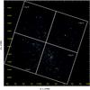 |
Fig. 1 True-color image of the young cluster NGC 1893. A kernel smoothing has been applied to highlight point sources. The energy bands of the RGB image are 0.5–1.1, 1.1–1.9, and 1.9–8.0 kev for red, green, and blue colors. Brightness is scaled to the logarithm of the photon number in the displayed pixel. The color model depicts zero flux as black. |
Starting from the Caramazza et al. (2008) catalog, we proceeded to the photon extraction of the source photons by means of Acis Extract1 (AE) v3.131 (Broos et al. 2002), an IDL-based package of tools that can assist the observer in performing the many tasks involved in analyzing a large number of point sources observed with the ACIS instrument on Chandra. AE makes extensive use of TARA2, a package of tools in the IDL language for visualizing and analyzing X-ray astronomical data in FITS format, CIAO3 (Fruscione et al. 2006), the data analysis system written for the needs of users of the Chandra X-ray Observatory, and FTOOLS4, a general package of software to manipulate FITS files.
The extraction of point sources performed with AE takes the point spread function (PSF) for single sources into account, which strongly depends on the off-axis distance (θ). While the PSF is narrow and approximately circular in the inner part of the field of view (θ ≲ 5′), it has a non-Gaussian shape at large off-axis, becoming broader and more asymmetric.
Moreover, AE calculates the shape of the model PSF at each source position (by means of the CIAO task mkpsf), considering also that the fraction of the PSF where photons are extracted depends on crowding. In this way, AE finds a compromise between having the largest PSF fraction (thus providing good photon statistics for further spectral and timing analysis) and having the best signal-to-noise ratio, not to mention the importance of avoiding the contamination from nearby sources.
After calculating the PSF shape, AE refines the initial source positions, in our case originally estimated by PWDetect (Damiani et al. 1997a) assuming a symmetric PSF, by correlating the source images with the model of local PSFs. Following AE science hints5, this last procedure was only used for those sources lying off-axis by greater than 5 arcmin (321 sources), while for the rest of the sources we simply adopt mean photon positions. Coordinates listed in Table 1, as well as their 1σ uncertainties, are the result of this process.
After recomputing positions, AE defines source extraction regions as polygonal contours of the model PSF containing a specified fraction of source events (fPSF). Generally, we chose fPSF = 90%, and computed the contours from the PSF for a monoenergetic source with E = 1.49 keV. For a few sources in the denser parts of the field of view this fraction was reduced so as to avoid contamination with other nearby sources, in the most extreme cases down to fPSF ~ 40%.
Although the ACIS-I instrumental background level is spatially quite uniform, the actual observed background varies substantially across the NGC 1893 field due to the extended PSF wings of bright sources and to their readout trails. Background was therefore estimated locally for each source, adopting once again the automated procedure implemented in AE, which defines background extraction regions as circular annuli with inner radii 1.1 times the maximum distance between the source and the 99% PSF contour, and outer radii defined so that the regions contains more than 100 “background” events. To exclude contamination of the regions by nearby sources, background events are defined from an image that excludes events within the inner annular radii of all the 1021 sources.
Results of the photon-extraction procedure are listed in Cols. 7–10 of Table 1, where we give the background-corrected extracted source counts for 0.5–8.0 keV, the associated error and the total background counts expected. In summary, our 1021 X-ray sources span a wide range of photon flux, from ~3 to ~7100 photons during the exposure time. Most sources are faint (e.g. 60% have fewer than 50 photons).
In the last six columns of Table 1, we list some characteristics of the sources: the significance (signal-to-noise ratio), Kolmogorov-Smirnov probability that the lightcurves of the sources are constant, the median photon energy, the absorption-corrected X-ray luminosities, and a flag indicating the method used to determine them.
NGC 1893 Chandra catalog: basic source properties.
3. Spectral analysis
To determine the intrinsic luminosity of our sources, spectral analysis is necessary. Unfortunately, spectral fitting can only be applied to high counts sources, while relatively faint sources with poor statistics cannot be investigated using this method.
To overcome this limit, we decided to perform spectral fitting (Sect. 3.1) on 311 sources for which it is possible to bin the spectrum so that, in the background-subtracted (net) spectrum, each rebinned channel achieves a signal-to-noise ratio of at least 3. In situations where the background level is high, this approach can produce higher quality binning compared to fixing a minimum number of counts in the source spectrum. For less intense sources we analyzed the spectrum of sources considering the quantiles of the distribution of energy for source counts. As we describe in the following for sources down to 30 counts, applying a quantile method (Hong et al. 2004), we have been able to derive the values of NH and kT interpolating directly from a thermal grid of models with good accuracy, while for very low statistics sources, we have used the quantile analysis to derive a median conversion factor from the count rate to the X-ray luminosity. Energy quantiles have been also used to discern the extragalactic contaminants.
3.1. Spectral fitting
Reduced source and background spectra in the 0.5–8.0 keV band have been produced with AE (see Sect. 2), along with individual “redistribution matrices files” (RMF) and “ancillary response files” (ARF). We fit our spectra by assuming emission by a thermal plasma, in collisional ionization equilibrium, as modeled by the APEC code (Smith et al. 2001). Elemental abundances are not easily constrained with low statistics spectra and were fixed at Z = 0.3 Z⊙ (see Prisinzano et al. 2011), with solar abundance ratios taken from Anders & Grevesse (1989). The choice of subsolar abundances is suggested by several X-ray studies of star-forming regions (e.g. Feigelson et al. 2002; Maggio et al. 2007). Absorption was accounted for using the WABS model, parametrized by the hydrogen column density, NH (Morrison & McCammon 1983).
We fit source spectra with one-temperature (1T) plasma models using an automated procedure. To reduce the risk of finding a relative minimum in the χ2 spaces, our procedure chooses the best fit among several obtained starting from a grid of initial values of the model parameters: log(NH) = 21.0, 22.0 cm-2, and kT = 0.5, 1.0, 2.0, 10.0 keV.
Among the 311 sources for which we conducted the spectral fitting, it was possible to determine NH and kT for 286 sources. Using the spectral fit parameters, we then derived X-ray luminosities for each of the 286 sources modeled with 1T spectrum, considering for NGC 1893 a distance of 3.6 kpc (Prisinzano et al. 2011). These sources are tagged with an “a” in Col. (16) in Table 1, and their luminosities are listed in Col. (15). The 25 sources for which we were unable to fit the spectra with a 1T model were analyzed with the study of the energy quantiles of the spectrum (see following sections).
3.2. Quantile analysis
Spectral fitting analysis cannot be applied to faint sources, but a rough analysis of the whole sample can be achieved by studying the median photon energy of each source. We plot in Fig. 2 the distribution of the source median energy computed in the [0.5–8.0] keV range. From this plot, we can retrieve some information about the population of our X-ray sources: the median value of the distribution is 1.6 keV, the bulk of the distribution is between 1 and 2 keV (62% of the median photon energy of the sources lies in this range), while 10% of the values are over 4 keV. This energetic tail of the distribution is probably due to extragalactic contaminants, even if we cannot exclude at this stage stellar flares on NGC 1893 members playing some role. While this kind of analysis is very helpful for understanding the behavior of the entire sample, it does not help much for characterizing of single sources.
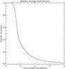 |
Fig. 2 Cumulative distribution function of the photon median energy of each source computed in the [0.5–8.0] keV range for all the sources. |
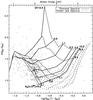 |
Fig. 3 Quantiles of X-ray spectra. The dots indicate the quantities derived from source energy quantiles. The two grids show the same quantities derived from simulated spectra. The solid line grid refers to thermal spectra with NH = [1020,1021,0.6 × 1022,1.1 × 1022,3.4 × 1022,6 × 1022] cm-2 and kT = [0.3,0.5,1.1,2.3,4.0,10.0] keV, and the dashed line grid to simulated power-law spectra typical of AGN, with the same NH values and power-law indices Γ = [0.0,0.4,1.0,1.6,2.0] . |
The conventional spectral classification of weak sources is often performed in the literature by means of the ratios of source counts in different spectral bands, i.e. X-ray hardness ratios (XHR) that can be considered “X-ray colors” (Schulz et al. 1989; Prestwich et al. 2003). The flaw in this method is that the choice of the bands is strongly related to the spectral shape and that, depending on the number of counts in each band, the error bar related to the ratio may be very large. For these reasons, we decided to apply an alternative method, introduced by Hong et al. (2004), which uses the energy value that divides photons into predetermined fractions, instead of the ratio of counts in prefixed bands. Following Hong et al. (2004), if Ex% is the energy below which the net counts are x% of the total counts, quantile Qx is  , where Elo and Eup are the lower and upper boundaries of the full energy band, i.e. 0.5 and 8.0 keV in our case. The fractions we choose are the median (50% quantile) and the quartiles (25% and 75% quantiles). Since quantiles are not independent for a given spectrum, Hong et al. (2004) selected the independent variables log (Q50/(1 − Q50)) and 3(Q25/Q75), in order to have information on the photon population in several portions of the spectrum. The derived quantile values will be compared with those calculated from simulated spectra in order to derive the best spectral parameters. Figure 3 shows the scatter plot of quantiles measured for our sources, compared with grids calculated from simulated spectra. The solid line grid refers to thermal spectra, and the dashed grid to power-law spectra, with spectral index typical of AGNs (Brandt et al. 2001). We note that, as expected, most of the sources lie in the thermal grid region. By interpolating the loci of our sources inside the thermal grid, it is possible to attribute values of NH and kT to each source and derive the intrinsic X-ray luminosity at the distance of NGC 1893. In Fig. 4 we compare the X-ray luminosity derived from the quantile analysis with that derived from spectral fitting for the brightest sources. The luminosities derived from spectral fitting are generally consistent with those derived from quantile analysis, and a linear regression between the two luminosities results in a coefficient 1.04 ± 0.4 giving strong support to the effectiveness of the method. The sources for which the luminosity was derived from the quantile analysis are indicated with a “b” in Col. (16) of Table 1.
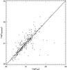 |
Fig. 4 Scatter plot of the X-ray luminsity derived from spectral fitting versus that derived from quantile analysis. The solid line indicates equal values of LX derived with the two methods. |
By analyzing the sources outside the region covered by the thermal grid, we found three subclasses of objects:
-
Two-temperature spectra. There is a small fraction of fairlystrong sources (between 30 and 50 photons) that lie over the leftbound of the thermal grid. Due to the concavity of the grid, this isthe locus where thermal spectra characterized by twotemperatures lie. For these cases, in our 1T approximation, weassociated them to the lowest NH curve, interpolating just the kT value, which depends basically on the median energy of the spectrum (see Fig. 3).
-
Very poor statistics spectra. Most of the sources outside the thermal grid are sources with fewer than 30 photons, with very large errors on quantiles. For these objects, we decided to adopt a single median conversion factor from count rate to luminosity. The conversion factor was derived from the quantile analysis of sources with more than 30 photons and applied to sources with fewer than 30 photons. These sources are indicated with a “c” in Col. (16) of Table 1.
-
Power-law spectra. A small fraction of the sources lie on the power-law grid and will be discussed in Sect. 3.2.1.
3.2.1. Rejecting extragalactic contaminants
As shown above, with the energy quantiles analysis, it is possible to attribute a luminosity value to each source in the sample. It is also useful to investigate the contaminant population in the sample. NGC 1893 lies toward the galactic anticenter, therefore we expect to detect a large number of extragalactic sources. Moreover, the long exposure needed to investigate the faint population of our distant cluster results in a high probability of detecting AGNs. To estimate the number of AGNs, we considered the sensitivity for three different off-axis regions in the Chandra ACIS-I field of view and calculated the minimum flux that we expect from a detected extragalactic source with a typical power-law index Γ = 1.4 (Brandt et al. 2001) in the direction of NGC 1893, (NH = 6.56 × 1021 cm-2, Dickey & Lockman 1990). By comparing the obtained fluxes with the log N-Log S obtained from the Chandra Deep Field North (Bauer et al. 2004), we expect to find ~ 190 AGNs among our sources.
From the diagram in Fig. 3, we find 128 sources that are outside the thermal grid and seem to be compatible with the power-law grid. We have tagged them as candidate AGNs in our catalog, but we have not excluded them from further analysis. Caution is needed because a very hard spectrum, due e.g. to flares, can be confused with a power-law spectrum; indeed, from the analysis of the variability, we have found that 16 sources tagged as candidate AGN show big flares. The spectral analysis finds support from the spatial distribution of candidate AGNs. Looking at Fig. 1, the morphology of the cluster is evident, and it is clear that the distribution of sources in the four instruments chips is not uniform. We compared the number of sources detected in each chip with the number of candidate AGNs. As we expected, the total number of sources is higher in chips I1 and I3, where the peak density of the cluster lies, while the spatial distribution of the candidate AGNs is different and not related to the spatial distribution of the cluster. Again, we note that the candidate AGNs that show flares follow the same space distribution of the cluster, therefore we treat this population with caution but do not exclude it from the sample. This analysis is summarized in Table 2.
Number of detected X-ray sources and AGN candidates in the 4 Chandra ACIS-I chips.
3.3. Upper limit to the X-ray luminosity of undetected NGC 1893 members
The purpose of the present work is to examine the X-ray properties of the NGC 1893 members, investigate the properties of stars in different evolutionary stages, and compare them with those of other star formation regions. For these reasons, we take advantage of the work described in Prisinzano et al. (2011) in which the optical and the infrared properties of NGC 1893 members are described. To compare the luminosity of stars from different classes without any bias due to different depths of infrared, X-ray and optical images, we derived upper limits to the X-ray luminosity for all the cluster members in Prisinzano et al. (2011) falling in the Chandra ACIS-I field of view and undetected in X-rays. Upper limits to the photon count rates were calculated with PWDetect (Damiani et al. 1997a,b), with a detection threshold significance set to 4.6σ, the same as used for source detection (Caramazza et al. 2008). To convert count rate upper limits into X-ray luminosity for X-ray undetected members, we calculated a conversion factor, considering the median value of the ratio between X-ray luminosity and count rate for the detected X-ray sources as done for the detected sources. In Table 3 we list the sequence number of the source in Prisinzano et al. (2011), along with the coordinates and the upper limit to the X-ray luminosity of the 158 X-ray undetected Class II members that we will analyze.
Upper limit to the X-ray luminosities for NGC1893 X-ray undetected members.
4. X-ray properties of low-mass members
Focusing on the X-ray properties of the NGC 1893 low-mass members, we started from the member catalog of Prisinzano et al. (2011). In particular, we selected all the Class II or Class III candidate members with mass lower than 2 M⊙ and whose optical colors are compatible with the cluster locus. To have a complete sample of sources, we selected all the stars with mass greater than 0.35 M⊙, the choice of this completeness threshold derives from analysis of the color-magnitude diagram (Fig. 11 in Prisinzano et al. 2011) and will be confirmed in the following. We also required that the candidate members are inside the Chandra ACIS-I field of view. In this way, we identify 591 low-mass members, 307 of which are Class II stars, while 284 are classified as Class III stars. Among the 591 members, 158 of the Class II stars are not detected in the X-ray observations, therefore we have only a determination of the upper limit to their X-ray luminosity. The following analysis is based on the sample of 591 low-mass members.
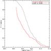 |
Fig. 5 Cumulative X-ray luminosity functions of the Class II and Class III members. The nondetections were taken into account, deriving the XLFs with the Kaplan-Meier maximum likelihood estimator. |
To compare the luminosity of different classes of objects, we analyzed the cumulative X-ray Luminosity Functions (XLF) of the Class II and Class III members. In order to take into account non-detections, XLFs were derived using the Kaplan-Meier maximum likelihood estimator (Kaplan & Meier 1958). Figure 5 shows the comparison of the cumulative X-ray luminosity functions of Class II and Class III members. Looking at this global description, we note that the range of luminosity is 3 × 1029−3 × 1031 erg s-1. It is evident that the Class III stars are brighter in X-rays, the median is higher and the body of the Class III object distribution is above that of Class II objects. At this age the dynamo mechanism is saturated in most of the PMS stars, therefore the X-ray luminosity scales as the bolometric luminosity of the star (e.g. Preibisch et al. 2005). This means that the difference in the whole XLF may be due to intrinsic properties or to a different bolometric luminosity (or mass) distribution among the two infrared classes. To avoid the mass dependence, it is usual to compare the XLFs in several ranges of mass (e.g. Flaccomio et al. 2003b; Preibisch et al. 2005; Prisinzano et al. 2008), despite the large errors caused by having few objects in each bin of mass. We overcome both of these difficulties by analyzing the Class II and Class III X-ray luminosities as a function of the bolometric luminosity of the star. Figure 6 shows the quantiles (25%, 50%, 75%) of the LX distribution in running intervals of bolometric luminosity covering 80 datapoints, for both of Class II (continuous line) and Class III (dashed line) stars. The resulting lines have been smoothed over scales of 0.1 in logarithm of bolometric luminosity. Note that for Class II stars the quartiles have been plotted only where the fraction of LX upper limits does not affect the calculation of the quartiles themselves (e.g., the first quartile may be calculated only if LX upper limits are less than 25%). The three quartiles give us different information about the distribution of LX: the first quartile of Class III objects is similar to that correspondent to Class II stars, but we are able to calculate this value only for a small fraction of Class II member, due to the high fraction of LX upper limits in the faint sample. The median and the third quartile, that describe the body and tail of the X-ray distributions respectively, show the same feature. They are lower for Class II members but the difference decreases with bolometric luminosity and for bright stars the quartiles are similar to those of Class III members.
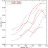 |
Fig. 6 X-ray luminosity distribution as a function of the stellar bolometric luminosity. The three couples of lines refer to the (25%, 50%, 75%) quartiles of the LX distributions calculated in running intervals of LBOL constituted by 80 contiguous points and smoothed in intervals of bolometric luminosity of 0.1 erg s-1. The continuous lines refer to Class II stars, the dashed ones to Class III stars. The quartiles have been plotted just where the fraction of upper limit values does not affect the calculation of the quartile itself. |
In order to interpret these results, we also need to compare the value of LX/LBOL for the two infrared classes of objects. We show in Fig. 7 the three running quartiles of the distribution of LX/LBOL for Class II and Class III objects. We see that the ratio decreases for the two classes as a function of LBOL. That means that the fraction of stars in the saturated dynamo regime (LX/LBOL ~ 3) decreases as a function of LBOL, and the displacement of Class II LX/LBOL below that for Class III stars means that the fraction of unsaturated X-ray sources is greater for disked stars than diskless ones.
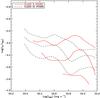 |
Fig. 7 LX/LBOL distribution as a function of LBOL. The three couples of lines refer to the (25%, 50%, 75%) quartiles of the LX/LBOL distributions calculated in running intervals of constituted by 80 contiguous points and smoothed in interval of bolometric luminosity of 0.1 erg s-1. The continuous line refer to Class II stars, and the dashed one to the Class III stars. |
We also compared the global X-ray properties of the stars in NGC 1893 with those of the Orion Nebula Cluster, in particular those obtained from the Chandra Orion Ultradeep Project (COUP) (Getman et al. 2005). As we discussed in Sect. 1, COUP gives the most complete set of studies in X-rays for young stars ever achieved for such a rich cluster; therefore, it has been considered a touchstone and its results compared with previous and successive X-ray studies. Feigelson & Getman (2005) compared the COUP XLF with that of NGC 1333 and IC 348 finding that “the shapes of different YSC XLFs appear to be remarkably similar to each other, once a richness-linked tail of high luminosity O stars is omitted”. Also RCW 38, IC 1396N, NGC 6357, the Carina Nebula Cluster, M 17, and NGC 2244 (Wolk et al. 2006; Getman et al. 2007; Wang et al. 2007; Sanchawala et al. 2007; Broos et al. 2007; Wang et al. 2008) compared the X-ray properties of several clusters to COUP results, demonstrating that in the Sun’s neighborhood the X-ray properties of star-forming regions are similar when comparing clusters of similar age and accounting for the IMF. The only relevant difference in the XLF is for Cep OB3b (Getman et al. 2006), where the XLF has a different shape than seen in the ONC with an excess at Log(LX) ~ 29.7 or 0.3 M⊙. The origin of the difference is not clear but could be ascribed to a deviation in the IMF or some other cause, such as sequential star formation generating a non-coeval population.
Starting from these previous results, we consider the ONC as representative of the X-ray properties of nearby star-forming regions and compare COUP results with those of NGC 1893, that is about ten times more distant from the Sun. Figure 8 describes the quantiles of the LX distributions for the Class II and Class III stars between 0.35 and 2 M⊙ for NGC 1893 and ONC. The first quantile of the NGC 1893 LX distributions is similar to the ONC, and since we know that the COUP sample is complete in this range of masses (Getman et al. 2005), it follows that our sample of stars has the same completeness as that of the ONC. The median of the two LX distributions are similar, but we note that the third quartile is larger for the ONC at the faintest LBOL. This means that we lack bright X-ray sources at the lowest masses in NGC 1893, and this cannot be related to an incompleteness of the sample: in that case we would lose faint stars so the effect would be enhanced. When comparing the X-ray properties of young stars in Cyg OB2 with those in the ONC, Albacete Colombo et al. (2007) note that dividing the COUP observation in 100 ks segments, a significant fraction of the longer and more energetic flares are missed. The difference between the two distributions could therefore be explained by COUP observation being longer than NGC 1893 ones, therefore in the ONC it is possible to observe rare, very energetic flares that, even when not modifying the median of the distribution, affect its tail. In order to consider the effect of the duration of the observation in the comparison of flares properties between NGC 1893 and the ONC (see Sect. 5), we normalize for the exposure time.
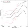 |
Fig. 8 X-ray luminosity distribution as a function of the bolometric luminosity. The three pairs of lines refer to the (25%, 50%, 75%) quartiles of the LX distributions calculated in running intervals of bolometric luminosity constituted by 80 contiguous points and smoothed in intervals of bolometric luminosity of 0.1 erg s-1. The continuous line refer to the NGC 1893 stars, and the dashed one to the ONC stars. |
5. X-ray variability
We have analyzed the variability of the lightcurves of the X-ray sources, by applying the Kolmogorov-Smirnov test to the arrival times of photons, and determined that 34% of our 1021 X-ray sources (including both members and non-members) are variable with a probability above 95%. If we restrict ourselves to only members, the variability fraction is 36%. When split according to whether a disk is present or not, 34% of the Class III stars are variable vs. 41% of Class II. While we cannot state that these two numbers are statistically different, we have to consider that Class II members are intrinsically fainter than Class III stars, and therefore the comparison has to be done by analyzing sources with the same statistics. Figure 9 shows the number of variable stars as a function of the minimum X-ray luminosity of the stars in the subsample. We note that, considering just the brightest stars, the discrepancy between Class II and Class III seems to be larger, suggesting a concrete difference in the fraction of variable stars in the two classes. It is interesting to investigate the behavior of Class II stars that still show accretion phenomena and those that do not present evidence of strong accretion. In the Prisinzano et al. (2011) catalog there is a subsample of Class II stars for which Hα photometry is available. Using that tracer (see Sect. 5.3 in Prisinzano et al. 2011, for details on selection), we singled out 50 Class II X-ray emitters with ongoing accretion, as indicated by Hα emission, and 77 that do not show strong Hα emission. The two samples of Class II X-ray emitters show the same fraction of variable light curves.
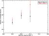 |
Fig. 9 Number of variable stars as a function of the minimum X-ray luminosity of the stars in the subsample. The vertical bars are the standard deviations ( |
A summary of the fraction of variable stars for the different subsamples of objects is given in Table 4.
The Kolmogorov-Smirnov test only gives a general indication of the variability of sources, but does not specify the nature of the variability. We therefore analyzed the lightcurves further in order to study the variability due to stellar flares. To single out flares in the lightcurves, we mapped the lightcurves using the maximum likelihood blocks (MLBs) (Wolk et al. 2005; Caramazza et al. 2007). The main characteristic of MLBs is that, being computed from the photon arrival times, their temporal length is not based on an a priori choice of temporal bin length, but depends on the light curve itself; for this reason MLBs are a useful tool in quantifying different levels of emission, and in detecting short impulsive events that might be missed by binning the lightcurves using fixed length bins. Applying the same operational definition of flares as is described in Caramazza et al. (2007) which takes both the amplitude and time derivative of the count rate into account, we singled out flares in the lightcurve as a sequence of blocks with a high count rate and a high rate of variation in the photon flux. We estimated the luminosity of each flare, scaling the total luminosity of the source during the observation by means of a count-rate-to-luminosity conversion factor. We then computed the energy of each flare, Eflr, by multiplying the flare luminosity for the flare duration, calculated as the total temporal length of the blocks associated with the flare. The results of this analysis are summarized in Table 4, where we state the number of flares per source with energy greater than 2 × 1035 erg (to be justified in the following).
X-ray variability for different subsamples of X-ray sources.
In Fig. 10, we show the number of flares per source as a function of the minimum X-ray luminosity of the analyzed subsample. Caramazza et al. (2007) demonstrated that the sensitivity of flare detection methods depends on source statistics, therefore it is interesting to compare the mean number of flares per source in several subsamples of sources, comprising sources with increasing luminosity. We note that for bright sources where we are able to detect all the flares, Class II stars are flaring significantly more than Class III stars and therefore that the disk plays an important role in generating this kind of high-energy events.
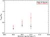 |
Fig. 10 Number of flare per source as a function of the minimum X-ray luminosity of the stars in the subsample. The vertical bars show the standard deviations as in Fig. 9. |
According to the microflares hypothesis, originally proposed for the solar case (see Hudson 1991), the X-ray emission of a star can be described as an ensemble of flares with a power-law energy distribution: 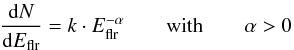 (1)where N is the number of flares with energies between Eflr and Eflr + dEflr, emitted in a given time interval. If the index of the power-law (α) is over 2, even very high levels of apparently quiescent coronal X-ray emission can be obtained from the integrated effects of many small flares. Figure 11 shows the cumulative distribution function (continuous line) of the intensity of flares for Class II and Class III members. For high counts the distribution is described by a power-law, but it progressively flattens towards low energies, most likely because not all low-count flares are individually detectable. Following the microflares hypothesis, we described the high-energy part of the differential distribution of flare counts as a power-law with index α. The cumulative distribution is then described by a power-law with index α − 1.
We determined the cutoff energy Ecut above which the observed distribution is compatible with a power-law and the relative index α − 1, with the same method as in Stelzer et al. (2007) (see also Crawford et al. 1970):
 In agreement with our assumption on power-law shape for the distribution, taking Ecut larger than the chosen cutoff, the best-fit value of α remains stable within the uncertainties, while we cannot neglect the incompleteness effect under this threshold.
Figure 11 also shows the cumulative distribution of flare energies for the Class II and Class III samples. We noticed that Class II star are more variable and more flaring than Class III objects, but we now see that the flares of Class II and Class III stars show the same distribution. We calculated the slope of the two power-laws, finding α − 1 = 1.4 ± 0.4 for the two subsamples.
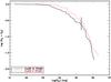 |
Fig. 11 Normalized cumulative distribution function of flare energies for Class III and Class II stars. In the range of energies above the cutoff value Ecut = 2 × 1035 erg (vertical segment), the two distributions are compatible with a power-law with α − 1 = 1.4 ± 0.4; for low counts the distributions flatten, most likely because the detection of low-counts flares is incomplete. |
Figure 12 shows the comparison between the cumulative distribution function of flare energies for NGC 1893 and the ONC. The distributions are normalized to the total number of sources of each sample and to the total exposure time. Above the completeness cutoff energy the two distributions are similar.
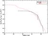 |
Fig. 12 Cumulative distribution function of flare energies for X-ray members in NGC 1893 (solid line) and ONC (dotted line). The distributions are normalized to the total number of sources of each sample and to the total exposure time. In the range of energies above the cutoff value Ecut = 2 × 1035 erg (vertical segment), where both the flare energy distributions are complete, the distributions of the flares follow similar distributions. |
Figure 13 shows the comparison between the mean number of flares for the NGC 1893 and the ONC samples. To compare the same kind of flares, we considered only the flares over the completeness cutoff energy. The number of flares per source is higher in the ONC but the difference decreases when we exclude low statistic sources. We infer that the difference may be due from a likely incompleteness of the NGC 1893 sample at low luminosities.
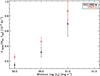 |
Fig. 13 Mean number of flares per kilosecond above the cutoff value Ecut = 2 × 1035 erg for subsamples of X-ray sources with LX higher than a given value. Circles refer to the NGC 1893 X-ray members, and diamonds to the ONC members. The vertical bars are the standard deviations as in Fig. 9. |
6. Discussion
The influence of the environment on star formation process may also be investigated through the analysis of X-ray emission. For its position in the Milky Way, NGC 1893 is a good target for investigating the possible differences in the behavior of stellar coronae and compare stars in clusters at the periphery of the Galaxy with those lying in dense spiral arms in the solar neighborhood.
We analyzed the X-ray properties of NGC 1893, in particular comparing the XLF of low-mass (<2 M⊙) Class II and Class III young stellar objects. We confirmed the known result that the classical T Tauri Stars (CTTS), i.e. the stars with signatures of disks, are globally less active than the weak-lined T Tauri stars (WTTS), i.e. stars that have no signatures of optically thick disks (e.g. Preibisch et al. 2005), while being more variable. We further investigated this result, by analyzing the behavior of LX as a function of the bolometric luminosity. The correlation between these variables is compatible with the well known saturated dynamo scenario, typical of pre-main sequence stars. Using the method described in Sect. 4, we demonstrated that, even considering stars with similar LBOL, the median LX is lower for Class II stars, even if the difference decreases for stars with high LBOL. Our statistical analysis suggests that the fraction of unsaturated Class II members is greater than for the Class III members. This result agrees with the scenario in which accretors stars are less luminous than non-accreting stars (Stelzer & Neuhäuser 2001; Flaccomio et al. 2003a; Stassun et al. 2004; Preibisch et al. 2005; Flaccomio et al. 2006; Telleschi et al. 2007). However, the reason Class II should be underluminous in X-rays is not well understood. There are four main ideas that have been formulated to explain the different behaviors of disked and diskless stars; two are related to the presence of disk itself and two to the presence of accretion from the disk.
-
1)
The lower X-ray luminosity of Class II starscould be related to the higher extinction due to X-ray absorptionby circumstellar disks, even if the COUP survey results do notsupport this idea (Preibischet al. 2005).
-
2)
A possible explanation is related to the magnetic braking: indeed, there are examples of magnetic connection between the star and the disk leading to the idea that disked stars are on average slower than diskless stars (Favata et al. 2005; Rebull et al. 2006; Prisinzano et al. 2008) and have a weaker dynamo action with consequent lower X-ray emission. In this case, the dynamo process would be the same for a star with and without disk and the lower luminosity of CTTS could be attributed to the slower rotation of CTTS related to the presence of the disk.
-
3)
The presence of accretion may alter the stellar structure and change the dynamo process itself (Preibisch et al. 2005), in this case the dynamo process could be different with different saturation limits for CTTS and WTTS.
-
4)
Finally, Gregory et al. (2007) demonstrate that the corona is not able to heat all the material in the accretion columns and this cooler material, not visible in X-rays may obscure the line of sight to the star, reducing the X-ray emission. Recently, this scenario was also supported by Flaccomio et al. (2010) who found a correlation between the X-ray and optical variability for CTTS, while they did not find any correlation for WTTS. With our sample of data, we are not able to prefer one of the previous hypotheses; however we can add the observational constraint that the difference between the two classes of object is more evident for low-mass stars and we can infer that this can be related to the different evolution time of disks around low-mass and solar-mass stars, leading to a larger fraction of disked stars at the lowest masses (Carpenter et al. 2006; Sicilia-Aguilar et al. 2006; Lada et al. 2006; Megeath et al. 2005).
We have also compared the X-ray properties of NGC 1893 with those of the ONC low-mass members. At this age the dynamo mechanism is saturated for a large fraction of the stars and this leads to a dependence by LX on the bolometric luminosity (e.g. Preibisch et al. 2005). Since we cannot a priori assume that the mass distribution in the two clusters is similar, we compared the two samples as a function of the bolometric luminosity. With this method, we found that the median of the two LX distributions vs. mass are similar, but the third quartile is larger for the ONC at the faintest LBOL. This effect seems to indicate an intrinsic lack of bright X-ray sources at the lowest masses in NGC 1893. This difference with the ONC cannot be an indication of the incompleteness of the NGC 1893 sample because, in that case, we would lose faint stars and the effect would be in the opposite direction. This difference between the two clusters in the high-luminosity tail of the LX distributions could be ascribed to the longer duration of COUP observation: indeed, in the ONC there was the possibility of observing long energetic flares that enhance the third quartile of the distribution.
Analyzing the variability of Class II and Class III stars in our sample, we find the familiar results that Class II are more variable than Class III stars and show more flares. The explanation of this behavior can be related to the effect of accretion. Flaccomio et al. (2010) observe that the X-ray variability of disked stars can come from the shielding of most of the coronal plasma by dense accretion streams of cold material (see Gregory et al. 2007). It is difficult to compare the variability of NGC 1893 sources with the Orion Nebula Cluster ones in detail, because of the several biases due to the different distance and the different duration of the X-ray observations that lead to a different completeness of the samples. Taking these several biases into account, we find that the X-ray flares in Orion and NGC 1893 show a similar energy distribution frequency, leading to the indistinguishable behavior of the two clusters from the coronal variability point of view.
We conclude that, despite its peculiar location in the Galaxy, NGC 1893 includes a rich population of Class II and Class III X-ray sources that have, both from the X-ray luminosity and X-ray variability point of view, similar properties to nearby star-forming regions, such as the ONC. That the X-ray properties of clusters in such different environments are so similar gives strong support to the Feigelson & Getman (2005) suggestion that the X-ray properties can be used as standard candles, providing a new instrument for measurement for distances of young clusters (Kuhn et al. 2010).
7. Summary and conclusion
As part of the large multiwavelength project The Initial Mass Function in the outer Galaxy: the star-forming region NGC 1893, we have analyzed the 450 ks Chandra Observations, and studied the X-ray properties of the 1021 detected sources. The X-ray data were combined to optical, near, and mid-infrared data (Prisinzano et al. 2011) in order to correlate the X-ray properties to the presence of disk and/or accretion. Below, we summarize the overall results of our investigations.
-
We derived the X-ray luminosity for our 1021 sources, tak-ing advantage of spectral fitting for 311 X-ray bright starsand of quantile analysis for the other sources, and found arange of X-ray luminosity 1029.5 − 1031.5 erg s-1. We analyzed, in particular,the low-mass stars X-ray luminosity taking the classifica-tion of candidate members in Class II andClass III members based on infrared excessesof Prisinzano et al. (2011) intoaccount. Class III stars appear intrinsically moreX-ray luminous than Class II stars, even whencomparing stars with the same bolometric luminosity. This maybe due to the presence of the “magnetically connected” disk itselfor to the ongoing accretion from the disk to the star.
-
We evaluated the variability of X-ray lightcurve using the Kolmogorov-Smirnov test, finding that 34% of the sources appear to be variable. We also searched for flares in our lightcurves and found 0.16 flares per source. We found that Class II stars are more variable and more flaring than Class III stars, while the flare energy properties are the same. This property may be related to the accreting cold material that obscures part of the X-ray emitting material, making accreting stars X-ray lightcurves more variable than the ones of diskless stars, but it also suggests that the presence of a disk plays a role in generating high-energy events.
-
Comparing the X-ray properties of NGC 1893 with those of the nearby star-forming region ONC, we found that the X-ray properties in NGC 1893 are not affected by the environment and that a stellar population in the outer Galaxy may have the same coronal properties of nearby star-forming regions. This provides strong evidence of the universality of the X-ray properties, and, as a consequence, a useful tool to determine properties, such as the distance or the total population, of young clusters.
Acknowledgments
This research made use of data obtained from the Chandra X-ray Observatory and software provided by the Chandra X-ray Center (CXC) in the application packages CIAO, ChIPS, and Sherpa. We acknowledge financial contributions from ASI-INAF agreement I/009/10/0, from the European Commission (contract N. MRTN-CT-2006-035890) and PRIN-INAF (P.I. Lanza). S.J.W. is supported by NASA contract NAS8-03060 (Chandra). We thank the referee for helpful suggestions and comments that improved this work.
References
- Albacete Colombo, J. F., Caramazza, M., Flaccomio, E., Micela, G., & Sciortino, S. 2007, A&A, 474, 495 [NASA ADS] [CrossRef] [EDP Sciences] [Google Scholar]
- Anders, E., & Grevesse, N. 1989, Geochim. Cosmochim. Acta, 53, 197 [Google Scholar]
- Bauer, F. E., Alexander, D. M., Brandt, W. N., et al. 2004, AJ, 128, 2048 [NASA ADS] [CrossRef] [Google Scholar]
- Brandt, W. N., Alexander, D. M., Hornschemeier, A. E., et al. 2001, AJ, 122, 2810 [NASA ADS] [CrossRef] [Google Scholar]
- Broos, P., Townsley, L., Getman, K., & Bauer, F. 2002, ACIS Extract, An ACIS Point Source Extraction Package, Pennsylvania State University [Google Scholar]
- Broos, P. S., Feigelson, E. D., Townsley, L. K., et al. 2007, ApJS, 169, 353 [NASA ADS] [CrossRef] [Google Scholar]
- Caramazza, M., Flaccomio, E., Micela, G., et al. 2007, A&A, 471, 645 [NASA ADS] [CrossRef] [EDP Sciences] [Google Scholar]
- Caramazza, M., Micela, G., Prisinzano, L., et al. 2008, A&A, 488, 211 [NASA ADS] [CrossRef] [EDP Sciences] [Google Scholar]
- Carpenter, J. M., Mamajek, E. E., Hillenbrand, L. A., & Meyer, M. R. 2006, ApJ, 651, L49 [NASA ADS] [CrossRef] [Google Scholar]
- Crawford, D. F., Jauncey, D. L., & Murdoch, H. S. 1970, ApJ, 162, 405 [NASA ADS] [CrossRef] [Google Scholar]
- Daflon, S., & Cunha, K. 2004, ApJ, 617, 1115 [NASA ADS] [CrossRef] [Google Scholar]
- Damiani, F., Maggio, A., Micela, G., & Sciortino, S. 1997a, ApJ, 483, 350 [NASA ADS] [CrossRef] [Google Scholar]
- Damiani, F., Maggio, A., Micela, G., & Sciortino, S. 1997b, ApJ, 483, 370 [NASA ADS] [CrossRef] [Google Scholar]
- Dickey, J. M., & Lockman, F. J. 1990, ARA&A, 28, 215 [NASA ADS] [CrossRef] [MathSciNet] [Google Scholar]
- Elmegreen, B. G. 1989, ApJ, 338, 178 [NASA ADS] [CrossRef] [Google Scholar]
- Elmegreen, B. G. 2002, ApJ, 577, 206 [NASA ADS] [CrossRef] [Google Scholar]
- Elmegreen, B. G. 2004, Mem. Soc. Astron. Ital., 75, 362 [NASA ADS] [Google Scholar]
- Ercolano, B., & Clarke, C. 2010, MNRAS, 402, 2735 [NASA ADS] [CrossRef] [Google Scholar]
- Favata, F., Flaccomio, E., Reale, F., et al. 2005, ApJS, 160, 469 [NASA ADS] [CrossRef] [Google Scholar]
- Feigelson, E. D., & Getman, K. V. 2005, in The Initial Mass Function 50 Year Later, ed. E. Corbelli, F. Palla, & H. Zinnecker (Dordrecht: Springer), Astrophysics Space Sci. Lib., 154, 163 [Google Scholar]
- Feigelson, E. D., Broos, P., Gaffney, J. A., et al. 2002, ApJ, 574, 258 [NASA ADS] [CrossRef] [Google Scholar]
- Fischer, D. A., & Valenti, J. 2005, ApJ, 622, 1102 [NASA ADS] [CrossRef] [Google Scholar]
- Flaccomio, E., Damiani, F., Micela, G., et al. 2003a, ApJ, 582, 398 [NASA ADS] [CrossRef] [Google Scholar]
- Flaccomio, E., Micela, G., & Sciortino, S. 2003b, A&A, 402, 277 [NASA ADS] [CrossRef] [EDP Sciences] [Google Scholar]
- Flaccomio, E., Micela, G., & Sciortino, S. 2006, A&A, 455, 903 [NASA ADS] [CrossRef] [EDP Sciences] [Google Scholar]
- Flaccomio, E., Micela, G., Favata, F., & Alencar, S. P. H. 2010, A&A, 516, L8 [NASA ADS] [CrossRef] [EDP Sciences] [Google Scholar]
- Fruscione, A., McDowell, J. C., Allen, G. E., et al. 2006, in SPIE Conf. Ser., 6270 [Google Scholar]
- Gaze, V. F., & Shajn, G. A. 1952, Izvestiya Ordena Trudovogo Krasnogo Znameni Krymskoj Astrofizicheskoj Observatorii, 9, 52 [Google Scholar]
- Getman, K. V., Flaccomio, E., Broos, P. S., et al. 2005, ApJS, 160, 319 [NASA ADS] [CrossRef] [Google Scholar]
- Getman, K. V., Feigelson, E. D., Townsley, L., et al. 2006, ApJS, 163, 306 [NASA ADS] [CrossRef] [Google Scholar]
- Getman, K. V., Feigelson, E. D., Garmire, G., Broos, P., & Wang, J. 2007, ApJ, 654, 316 [NASA ADS] [CrossRef] [Google Scholar]
- Gould, A., Flynn, C., & Bahcall, J. N. 1998, ApJ, 503, 798 [Google Scholar]
- Gregory, S. G., Wood, K., & Jardine, M. 2007, MNRAS, 379, L35 [NASA ADS] [CrossRef] [Google Scholar]
- Hong, J., Schlegel, E. M., & Grindlay, J. E. 2004, ApJ, 614, 508 [NASA ADS] [CrossRef] [Google Scholar]
- Hudson, H. S. 1991, Sol. Phys., 133, 357 [Google Scholar]
- Kaplan, E. L., & Meier, P. 1958, J. Amer. Statist. Assn., 457 [Google Scholar]
- Kuhn, M. A., Getman, K. V., Feigelson, E. D., et al. 2010, ApJ, 725, 2485 [NASA ADS] [CrossRef] [Google Scholar]
- Lada, C. J., Muench, A. A., Luhman, K. L., et al. 2006, AJ, 131, 1574 [NASA ADS] [CrossRef] [Google Scholar]
- Mac Low, M.-M., & Klessen, R. S. 2004, Rev. Mod. Phys., 76, 125 [NASA ADS] [CrossRef] [Google Scholar]
- Maggio, A., Flaccomio, E., Favata, F., et al. 2007, ApJ, 660, 1462 [NASA ADS] [CrossRef] [Google Scholar]
- Marco, A., & Negueruela, I. 2002, A&A, 393, 195 [NASA ADS] [CrossRef] [EDP Sciences] [Google Scholar]
- Mathis, J. S., Mezger, P. G., & Panagia, N. 1983, A&A, 128, 212 [NASA ADS] [Google Scholar]
- Megeath, S. T., Hartmann, L., Luhman, K. L., & Fazio, G. G. 2005, ApJ, 634, L113 [NASA ADS] [CrossRef] [Google Scholar]
- Morrison, R., & McCammon, D. 1983, ApJ, 270, 119 [NASA ADS] [CrossRef] [Google Scholar]
- Padoan, P., & Nordlund, Å. 1999, ApJ, 526, 279 [NASA ADS] [CrossRef] [Google Scholar]
- Pizzolato, N., Ventura, P., D’Antona, F., et al. 2001, A&A, 373, 597 [NASA ADS] [CrossRef] [EDP Sciences] [Google Scholar]
- Prestwich, A. H., Irwin, J. A., Kilgard, R. E., et al. 2003, ApJ, 595, 719 [NASA ADS] [CrossRef] [Google Scholar]
- Preibisch, T., Kim, Y., Favata, F., et al. 2005, ApJS, 160, 401 [NASA ADS] [CrossRef] [Google Scholar]
- Prisinzano, L., Micela, G., Flaccomio, E., et al. 2008, ApJ, 677, 401 [NASA ADS] [CrossRef] [Google Scholar]
- Prisinzano, L., Sanz-Forcada, J., Micela, G., et al. 2011, A&A, 527, A77 [NASA ADS] [CrossRef] [EDP Sciences] [Google Scholar]
- Rebull, L. M., Stauffer, J. R., Megeath, S. T., Hora, J. L., & Hartmann, L. 2006, ApJ, 646, 297 [NASA ADS] [CrossRef] [Google Scholar]
- Reylé, C., & Robin, A. C. 2001, A&A, 373, 886 [NASA ADS] [CrossRef] [EDP Sciences] [Google Scholar]
- Rolleston, W. R. J., Smartt, S. J., Dufton, P. L., & Ryans, R. S. I. 2000, A&A, 363, 537 [NASA ADS] [Google Scholar]
- Sanchawala, K., Chen, W.-P., Lee, H.-T., et al. 2007, ApJ, 656, 462 [NASA ADS] [CrossRef] [Google Scholar]
- Santos, N. C., Israelian, G., & Mayor, M. 2003, in The Future of Cool-Star Astrophysics: 12th Cambridge Workshop on Cool Stars, Stellar Systems, and the Sun, 2001 July 30–August 3, ed. A. Brown, G. M. Harper, & T. R. Ayres, University of Colorado, 12, 148 [Google Scholar]
- Sanz-Forcada, J., Prisinzano, L., Micela, G., Caramazza, M., & Sciortino, S. 2011, submitted [Google Scholar]
- Schulz, N. S., Hasinger, G., & Truemper, J. 1989, A&A, 225, 48 [NASA ADS] [Google Scholar]
- Sharma, S., Pandey, A. K., Ojha, D. K., et al. 2007, MNRAS, 380, 1141 [NASA ADS] [CrossRef] [Google Scholar]
- Shu, F. H., Adams, F. C., & Lizano, S. 1987, ARA&A, 25, 23 [Google Scholar]
- Sicilia-Aguilar, A., Hartmann, L., Calvet, N., et al. 2006, ApJ, 638, 897 [NASA ADS] [CrossRef] [Google Scholar]
- Smith, R. K., Brickhouse, N. S., Liedahl, D. A., & Raymond, J. C. 2001, ApJ, 556, L91 [NASA ADS] [CrossRef] [Google Scholar]
- Snell, R. L., Carpenter, J. M., & Heyer, M. H. 2002, ApJ, 578, 229 [NASA ADS] [CrossRef] [Google Scholar]
- Stassun, K. G., Ardila, D. R., Barsony, M., Basri, G., & Mathieu, R. D. 2004, AJ, 127, 3537 [NASA ADS] [CrossRef] [Google Scholar]
- Stelzer, B., & Neuhäuser, R. 2001, A&A, 377, 538 [NASA ADS] [CrossRef] [EDP Sciences] [Google Scholar]
- Stelzer, B., Flaccomio, E., Briggs, K., et al. 2007, A&A, 468, 463 [NASA ADS] [CrossRef] [EDP Sciences] [Google Scholar]
- Telleschi, A., Güdel, M., Briggs, K. R., Audard, M., & Palla, F. 2007, A&A, 468, 425 [Google Scholar]
- Vallenari, A., Richichi, A., Carraro, G., & Girardi, L. 1999, A&A, 349, 825 [NASA ADS] [Google Scholar]
- Wang, J., Townsley, L. K., Feigelson, E. D., et al. 2007, ApJS, 168, 100 [NASA ADS] [CrossRef] [Google Scholar]
- Wang, J., Townsley, L. K., Feigelson, E. D., et al. 2008, ApJ, 675, 464 [NASA ADS] [CrossRef] [Google Scholar]
- Wilson, T. L., & Matteucci, F. 1992, A&ARv, 4, 1 [NASA ADS] [CrossRef] [Google Scholar]
- Wolk, S. J., Harnden, F. R., Flaccomio, E., et al. 2005, ApJS, 160, 423 [NASA ADS] [CrossRef] [Google Scholar]
- Wolk, S. J., Spitzbart, B. D., Bourke, T. L., & Alves, J. 2006, AJ, 132, 1100 [NASA ADS] [CrossRef] [Google Scholar]
- Wouterloot, J. G. A., Brand, J., Burton, W. B., & Kwee, K. K. 1990, A&A, 230, 21 [NASA ADS] [Google Scholar]
- Yasui, C., Kobayashi, N., Tokunaga, A. T., Saito, M., & Tokoku, C. 2009, ApJ, 705, 54 [NASA ADS] [CrossRef] [Google Scholar]
All Tables
Number of detected X-ray sources and AGN candidates in the 4 Chandra ACIS-I chips.
All Figures
|
Fig. 1 True-color image of the young cluster NGC 1893. A kernel smoothing has been applied to highlight point sources. The energy bands of the RGB image are 0.5–1.1, 1.1–1.9, and 1.9–8.0 kev for red, green, and blue colors. Brightness is scaled to the logarithm of the photon number in the displayed pixel. The color model depicts zero flux as black. |
| In the text | |
|
Fig. 2 Cumulative distribution function of the photon median energy of each source computed in the [0.5–8.0] keV range for all the sources. |
| In the text | |
|
Fig. 3 Quantiles of X-ray spectra. The dots indicate the quantities derived from source energy quantiles. The two grids show the same quantities derived from simulated spectra. The solid line grid refers to thermal spectra with NH = [1020,1021,0.6 × 1022,1.1 × 1022,3.4 × 1022,6 × 1022] cm-2 and kT = [0.3,0.5,1.1,2.3,4.0,10.0] keV, and the dashed line grid to simulated power-law spectra typical of AGN, with the same NH values and power-law indices Γ = [0.0,0.4,1.0,1.6,2.0] . |
| In the text | |
|
Fig. 4 Scatter plot of the X-ray luminsity derived from spectral fitting versus that derived from quantile analysis. The solid line indicates equal values of LX derived with the two methods. |
| In the text | |
|
Fig. 5 Cumulative X-ray luminosity functions of the Class II and Class III members. The nondetections were taken into account, deriving the XLFs with the Kaplan-Meier maximum likelihood estimator. |
| In the text | |
|
Fig. 6 X-ray luminosity distribution as a function of the stellar bolometric luminosity. The three couples of lines refer to the (25%, 50%, 75%) quartiles of the LX distributions calculated in running intervals of LBOL constituted by 80 contiguous points and smoothed in intervals of bolometric luminosity of 0.1 erg s-1. The continuous lines refer to Class II stars, the dashed ones to Class III stars. The quartiles have been plotted just where the fraction of upper limit values does not affect the calculation of the quartile itself. |
| In the text | |
|
Fig. 7 LX/LBOL distribution as a function of LBOL. The three couples of lines refer to the (25%, 50%, 75%) quartiles of the LX/LBOL distributions calculated in running intervals of constituted by 80 contiguous points and smoothed in interval of bolometric luminosity of 0.1 erg s-1. The continuous line refer to Class II stars, and the dashed one to the Class III stars. |
| In the text | |
|
Fig. 8 X-ray luminosity distribution as a function of the bolometric luminosity. The three pairs of lines refer to the (25%, 50%, 75%) quartiles of the LX distributions calculated in running intervals of bolometric luminosity constituted by 80 contiguous points and smoothed in intervals of bolometric luminosity of 0.1 erg s-1. The continuous line refer to the NGC 1893 stars, and the dashed one to the ONC stars. |
| In the text | |
|
Fig. 9 Number of variable stars as a function of the minimum X-ray luminosity of the stars in the subsample. The vertical bars are the standard deviations ( |
| In the text | |
|
Fig. 10 Number of flare per source as a function of the minimum X-ray luminosity of the stars in the subsample. The vertical bars show the standard deviations as in Fig. 9. |
| In the text | |
|
Fig. 11 Normalized cumulative distribution function of flare energies for Class III and Class II stars. In the range of energies above the cutoff value Ecut = 2 × 1035 erg (vertical segment), the two distributions are compatible with a power-law with α − 1 = 1.4 ± 0.4; for low counts the distributions flatten, most likely because the detection of low-counts flares is incomplete. |
| In the text | |
|
Fig. 12 Cumulative distribution function of flare energies for X-ray members in NGC 1893 (solid line) and ONC (dotted line). The distributions are normalized to the total number of sources of each sample and to the total exposure time. In the range of energies above the cutoff value Ecut = 2 × 1035 erg (vertical segment), where both the flare energy distributions are complete, the distributions of the flares follow similar distributions. |
| In the text | |
|
Fig. 13 Mean number of flares per kilosecond above the cutoff value Ecut = 2 × 1035 erg for subsamples of X-ray sources with LX higher than a given value. Circles refer to the NGC 1893 X-ray members, and diamonds to the ONC members. The vertical bars are the standard deviations as in Fig. 9. |
| In the text | |
Current usage metrics show cumulative count of Article Views (full-text article views including HTML views, PDF and ePub downloads, according to the available data) and Abstracts Views on Vision4Press platform.
Data correspond to usage on the plateform after 2015. The current usage metrics is available 48-96 hours after online publication and is updated daily on week days.
Initial download of the metrics may take a while.