| Issue |
A&A
Volume 538, February 2012
|
|
|---|---|---|
| Article Number | A57 | |
| Number of page(s) | 12 | |
| Section | Interstellar and circumstellar matter | |
| DOI | https://doi.org/10.1051/0004-6361/201015999 | |
| Published online | 01 February 2012 | |
AKARI observations of ice absorption bands towards edge-on young stellar objects
1
Department. of Earth and Planetary SciencesKobe University,
657-8501
Kobe,
Japan
e-mail: This email address is being protected from spambots. You need JavaScript enabled to view it.
2
Department of Astronomy, School of Science, University of
Tokyo, 7-3-1 Hongo, Bunkyo-ku,
113-0033
Tokyo,
Japan
3
National Astronomical Observatory of Japan,
Osawa 2-21-1, Mitaka, 181-8588
Tokyo,
Japan
4
Department of Physics, Scottish Universities Physics Alliance
(SUPA), University of Strathclyde, Glasgow G4
ONG,
UK
5
Space Telescope Science Institute, 3700 San Martin Drive, Baltimore, MD
21218,
USA
6
Department of Physics, Nagoya University,
Furo-cho, Chikusa-ku, 464-8602
Nagoya,
Japan
7
Institute of Space and Astronautical Science, Japan Aerospace Exploration Agency,
3-1-1
Yoshinodai, Sagamihara, 229-8510
Kanagawa,
Japan
Received: 26 October 2010
Accepted: 17 November 2011
Abstract
Context. Circumstellar disks and envelopes of low-mass young stellar objects (YSOs) contain significant amounts of ice. Such icy material will evolve to become volatile components of planetary systems, such as comets in our solar system.
Aims. To investigate the composition and evolution of circumstellar ice around low-mass young stellar objects (YSOs), we observed ice absorption bands in the near infrared (NIR) towards eight YSOs ranging from class 0 to class II, among which seven are associated with edge-on disks.
Methods. We performed slit-less spectroscopic observations using the grism mode of the InfraRed Camera (IRC) on board AKARI, which enables us to obtain full NIR spectra from 2.5 μm to 5 μm, including the CO2 band and the blue wing of the H2O band, which are inaccessible from the ground. We developed procedures to carefully process the spectra of targets with nebulosity. The spectra were fitted with polynomial baselines to derive the absorption spectra. The molecular absorption bands were then fitted with the laboratory database of ice absorption bands, considering the instrumental line profile and the spectral resolution of the grism dispersion element.
Results. Towards the class 0-I sources (L1527, IRC-L1041-2, and IRAS 04302), absorption bands of H2O, CO2, CO, and XCN are clearly detected. Column density ratios of CO2 ice and CO ice relative to H2O ice are 21−28% and 13−46%, respectively. If XCN is OCN−, its column density is as high as 2−6% relative to H2O ice. The HDO ice feature at 4.1 μm is tentatively detected towards the class 0-I sources and HV Tau. Non-detections of the CH-stretching mode features around 3.5 μm provide upper limits to the CH3OH abundance of 26% (L1527) and 42% (IRAS 04302) relative to H2O. We tentatively detect OCS ice absorption towards IRC-L1041-2. Towards class 0-I sources, the detected features should mostly originate in the cold envelope, while CO gas and OCN− could originate in the region close to the protostar, where there are warm temperatures and UV radiation. We detect H2O ice band towards ASR41 and 2MASSJ 1628137-243139, which are edge-on class II disks. We also detect H2O ice and CO2 ice towards HV Tau, HK Tau, and UY Aur, and tentatively detect CO gas features towards HK Tau and UY Aur.
Key words: circumstellar matter / infrared: ISM / stars: formation / astrochemistry
© ESO, 2012
1. Introduction
In molecular clouds, protostellar envelopes, and protoplanetary disks, significant amounts of oxygen and carbon are in the form of molecules in ice mantles, such as H2O, CO, CO2, and CH3OH (e.g. Whittet 1993; Murakawa et al. 2000; Gibb et al. 2004). These interstellar ices are formed by the adsorption of gas-phase molecules onto grain surfaces and/or the grain-surface reactions of the adsorbed species (e.g. Aikawa et al. 2005).
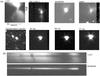 |
Fig. 1 a) Images of our targets taken by AKARI with the N3 filter (2.7−3.8 μm). The stellar light is dispersed from right (short wavelength) to left (long wavelength). The FOV is 1′ × 1′. The coordinate at the center of the FOV is listed in Table 1. Images of IRC-L1041-2 and 2MASS J1628137-243139 are damaged by cosmic rays, while images of HV Tau, HK Tau, ASR41, and UY Aur are affected by saturation and column pull down. b) Spectral images of 1527 and IRAS 04302. |
Ices in circumstellar disks of low-mass young stellar objects are of special interest as they contribute to the raw material of planetary formation. Observations of disk ices, however, are not straightforward for the following two reasons, and thus remain limited in number. Firstly, ices exist mostly near the midplane at r ≥ several AU. Observations of disk ices are basically restricted to edge-on disks, where the ice bands absorb stellar light, scattered stellar light, and/or thermal emission of warm dust in the disk inner radius (Pontoppidan et al. 2005). The targets are naturally heavily extincted by dust, and thus are faint. Secondly, it is unclear whether the ice absorption bands, if detected, originate in the disk or other foreground components (i.e. ambient clouds). The source CRBR 2422.8-3423 was the first edge-on object towards which detailed ice observations were performed (Thi et al. 2002). Pontoppidan et al. (2005) concluded, via detailed analysis and modeling of the object, that only a limited amount (<20%) of detected CO ice may exist in the disk, while up to 50% of water and CO2 may originate in the disk. They also found that the 6.85 μm band, which is tentatively attributed to  , has a prominent red wing. Since this wing is reproduced by the thermal processing in the laboratory, it indicates that along the line of sight towards CRBR 2422.8-3423 there is warm ice in the disk.
Honda et al. (2009) succeeded in detecting water ice in a disk around a Herbig Ae star, which is not edge-on. They observed scattered light from a disk around HD142527 at multiple wavelength bands around ~3 μm. This method can be a powerful tool for investigating the spatial distribution of ices in disks. However, it would currently be difficult to detect ice features other than the 3 μm water band via scattered light.
In the present paper, we report near infrared (NIR) (2.5−5 μm) observations of edge-on disks using the grism mode of the IRC on board AKARI. We selected seven edge-on YSOs; three are considered to be in a transient state of class 0-I, and four are class II (see Sect. 2 for more detailed descriptions). Although the absorption by the protostellar envelope may overwhelm the absorption by the disk in class 0-I YSOs, envelope material along our line of sight (perpendicular to the rotation axis and outflow) is likely to end up in the midplane region of the forming disk, and ices with a sublimation temperature of >50 K (i.e. CO2 and H2O) would survive the accretion shock onto the disk (Visser et al. 2009).
Ice observations towards low-mass YSOs have been performed using Spitzer Space Telescope (SST) and various ground-based telescopes such as the Very Large Telescope (VLT) and Subaru. Pontoppidan et al. (2003a) observed the 4.67 μm CO ice band, which is observable from the ground, towards 39 YSOs. Using SST, Furlan et al. (2008) and Pontoppidan et al. (2008) observed the strong CO2 ice band at 15.3 μm towards class I sources. Observations with SST also detected absorption bands of CH3OH, HCOOH, H2CO, and CH4 (Boogert et al. 2008; Zasowski et al. 2009; Öberg et al. 2008). Since ground-based observations are restricted to atmospheric windows, and since SST is restricted to the mid infrared (5−36 μm), NIR observations via AKARI are important to comprehend the full spectra of ices in circumstellar material. AKARI has a high enough sensitivity for the spectroscopic observation of low-mass YSOs; the sensitivity of the AKARI grism mode at 3 μm is 120 μJy (1σ, 10 min), which is almost comparable to the K-band sensitivity of the spectroscopic observation at 8-m ground-based telescopes (VLT and Subaru). While the L-band sensitivity on the ground is ~5 mag or 100 times worse than at K-band, the sensitivity of the AKARI grism mode does not vary significantly at 2.5−4 μm, and only gradually worsens at longer wavelengths, by up to a factor of 3–4 at 5 μm.
Target list.
2. Observations
Observations were performed using the IRC (Onaka et al. 2007; Ohyama et al. 2007) on board the AKARI satellite (Murakami et al. 2007) from September 2006 to March 2007. We used the Astronomical Observational Template 04 (AOT04), designed for spectroscopy. The AOT04 replaces the imaging filters with transmission-type dispersers on the filter wheels to take near- and mid-infrared spectra. The field of view (FOV) consists of a 1′ × 1′ aperture (covered by 40 × 40 pixels in the imaging mode) (Fig. 1a) and a 10′ × 10′ aperture. The targets are set at the center of the 1′ × 1′ aperture (without a slit), where only the NIR channel is available. The resolving power of the IRC grism mode is 0.00965 μm/pixel, and the full-width at half maximum (FWHM) of the point spread function (PSF) is ~2.9 pixels in the NIR. The spectral resolution is thus ~100, which is sufficient to detect the ice absorption bands. In each observation, the following data are taken in a period of 600 s: two dark frames, one image frame with the N3 filter (2.7−3.8 μm), and eight slitless spectral images.
Table 1 lists our targets, and Fig. 1a shows the N3 images of our targets. The stellar light is dispersed from right (short wavelengths) to left (long wavelengths). The position angle of the FOV is fixed; the dispersion direction is almost aligned with the ecliptic latitude. The nebulosity of our targets extends almost perpendicularly to the dispersion direction. As an example, the spectral images of L1527 and IRAS 04302 are shown in Fig. 1b.
Both IRAS 04302 and L1527 (IRAS 04368+2557) are edge-on YSOs in a transient state from class 0 to class I (André et al. 2000). The YSO L1527 is of special interest from a chemical point of view; it is one of two YSOs where high abundances of carbon-chain species are observed. Carbon chains are considered to be formed by warm carbon-chain chemistry (WCCC): gas-phase reactions of sublimated CH4 (Sakai et al. 2008; Aikawa et al. 2008). The large organic species detected towards several low-mass YSOs (e.g. IRAS 16293) are not, however, detected towards L1527 (Sakai et al. 2008). Since the large organic species are formed from CH3OH, while carbon chains are formed from CH4, it is important to investigate ice bands, including the C-H bands, towards L1527, to determine whether its ice composition significantly differs from those of other low-mass YSOs.
The YSO IRC-L1041-2 was initially in our target list of background stars (i.e. field stars behind molecular clouds) (Noble et al., in prep.). The N3 image shows a faint object with nebulosity, which is similar to L1527. The SST observations also detected a YSO with nebulosity (T. L. Bourke, priv. comm.). The presence of a dark dust lane indicates that the YSO has a high inclination, close to edge-on.
The YSOs 2MASS J1628137 and ASR41 are edge-on class II objects. 2MASS J1628137 is accompanied by a tenuous (4 × 10⁻⁴ M⊙) envelope (Grosso et al. 2003). Hodapp et al. (2004) performed detailed modeling of the scattering and radiative transfer of ASR41 and concluded that the K-band image can be well reproduced by a protoplanetary disk embedded in a low-density cloud.
HK Tau B and HV Tau C are edge-on class II objects, in the HK Tau binary and HV Tau triplet systems, respectively. We initially aimed to obtain spectra of these edge-on objects, but the spectra were found to be contaminated and dominated by the bright primaries, because the binary separations are small (see Sects. 4.1 and 5). The ice absorption features towards HK Tau B and HV Tau C might still be observable, although the derivation of ice column densities is not straightforward. For a comparison with disks that are not edge-on, we also observed UY Aur, which is a binary system with a separation of 0.9′′ accompanied by a circumbinary disk. The inclination of the disk is ~42° (Hioki et al. 2007).
3. Data reduction and analysis
3.1. Reduction of the spectral image
The reduction pipeline provided by the AKARI project team, IRC_SPECRED (Ohyama et al. 2007), is unsuitable for our targets, because it automatically defines the area surrounding selected sources as “sky”, an area that is often contaminated by nebulosity in our observations.
To derive spectra from the data, we developed our own procedure, referring to the reduction method by Sakon et al. (2007). Firstly, we made a cosmic-ray-free dark for each target by taking the median of three dark frames; two dark frames were taken during the observation of each target, and one additional dark frame was taken from the preceding or subsequent observation in the AKARI archive. This procedure was necessary, because some frames are heavily damaged by cosmic rays. The dark was subtracted from the N3 image and spectral images.
The eight spectral images were slightly shifted in relation to each other by the attitude drift of the satellite. The task IRC_SPECRED measures the shift of each image relative to the fourth image. Referring to this measurement, we selected images with a relative shift of within 0.5 pixels, in both spatial and spectral directions. Images with larger shifts were discarded. Cosmic rays were removed by subtracting the median of the possible combinations of three frames from the selected frames. We then stack and average these cosmic-ray-free spectral images.
The local-sky region was selected by carefully avoiding nebulosity, field stars, and bad pixels. In the case of L1527, there is no “sky” region, because the nebulosity extends all over the 1′ × 1′ aperture (Fig. 1). Since we performed slitless spectroscopy, the spectral image of the nebulosity is a convolution of the nebula spectrum with the brightness distribution, and should not be considered as “sky”. We selected from the AKARI archive a 1′ × 1′ spectral image that can be used as sky; i.e. a dark region observed at a similar period and coordinate to those of L1527.
After the sky subtraction, we defined the spectrum region of each star in the spectral image, referring to the coordinates of the objects and the N3 image. The signal was integrated over eight pixels (12 arcsec) in the spatial direction. As an alternative approach, Noble et al. (in prep.) fit the signal at each wavelength with the PSF and integrated the signal. We confirmed that the result of the eight-pixel integration agrees well with this more sophisticated approach. We note that the spectrum is not perfectly aligned with the rows of the pixels. We adopted the formulation as the tilt of the spectrum  (1)where X and Y are the pixel number in the dispersion direction and spatial direction respectively, and Y0 is the center of the spectrum at an arbitrary position, X0, in the dispersion direction.
In Fig. 1, nebulosity is clearly seen towards L1527, IRC-L1041-2, IRAS 04302, and ASR 41. For these objects, we set Y0 in Eq. (1) as the brightest position in the spatial direction at a wavelength (X0) in the spectrum image, and integrated the spectrum over eight pixels in the spatial direction at each wavelength (Fig. 1). One exception is L1527; since the central point-like source is apparent and fainter than the nebulosity, we set Y0 as the central (faintest) position in the spatial direction, and integrated the signal over four pixels in the spatial direction (Fig. 1).
The integrated signal was divided by the aperture correction factor and response function before being converted into a spectrum. The response function was determined by the observation of a standard star (KF09T1). Wavelength calibration was done by the AKARI project team using the slit spectroscopy observation of standard stars. In our observations, we determined the wavelength of the spectrum by measuring the shift between the slit and the direct light position of the target in the N3 image.
According to the IRC team, the pixel-wavelength relation is a linear function. This linear correlation is confirmed in the wavelength range 2.5–4.5 μm, although the calibration is less certain at longer wavelengths. The CO absorption peak (~4.67 μm) is shifted to shorter wavelengths by 1–2 pixels in our data. Since similar shifts in this wavelength are reported in other IRC data, we shifted the data at ≥4.5 μm by 1–2 pixels towards longer wavelengths.
The error in flux was evaluated as follows. Firstly, we estimated the noise level in the “sky” region and converted it into an error in flux using the response function. Secondly, we estimated the flux errors caused by the wavelength assignment; we calculated fluxes by assuming that the shift between the slit and the direct light position of the target is 0.5 pixels larger/smaller. We then adopted the maximum of these errors.
3.2. Absorption features
To evaluate the ice absorption profile quantitatively, we normalized the spectrum with the continuum, which is assumed to be a second order polynomial, and was determined by referring to the three wavelength regions ~2.6 μm, 3.4−3.8 μm, and 4.2−4.9 μm. The choice of wavelengths differed slightly among objects to ensure a good fit to all spectra.
Template absorption profiles were obtained from “data base 2007” at Raymond & Beverly Sackler Laboratory for Astrophysics1. The database summarizes the absorption profiles of ice species measured in laboratories. Gerakines et al. (1995, 1996) measured the profiles and determined band strengths of various astrophysical ice analogs. From the database of Gerakines et al. (1995, 1996), we adopted profiles of pure ices at 10 K unless otherwise stated. In reality, interstellar ice is a mixture of various components such as H2O, CO, and CO2, and the peak position and shape of the absorption features change with the abundance ratio of the components. However, our spectral resolution is insufficiently high to perform such a detailed analysis of the ice mixture.
The profiles of the 4.27 μm CO2 band and the 4.67 μm CO band depend strongly on grain shape (Ehrenfreund et al. 1997). We adopted the continuously distributed ellipsoids (CDE) grain model for the CO band feature (Ehrenfreund et al. 1997; Boogert et al. 2002; Pontoppidan et al. 2003a). For the CO2 band, on the other hand, we adopted the spectrum of Gerakines et al. (1995), which is uncorrected for the grain shape, since it gives a good fit to our observational data. The pure CO2 feature with grain-shape (CDE) corrections agrees with neither our data nor the CO2 ice feature observed by ISO towards high-mass YSOs, which indicates that CO2 ice is not pure in interstellar medium. The ISO observations of the 4.27 μm feature indicated that the CO2 ice is primarily in a polar (H2O-rich) component of the ices (Whittet et al. 1998). However, to interpret our observation, we also need to introduce an apolar component to reproduce the blue wing at ~4.2 μm. Since our spectral resolving power is low, we simply use the spectrum of Gerakines et al. (1995) as a template, rather than combining multiple components of ice mixture with grain shape corrections. We also adopted the 3.05 μm H2O band of Gerakines et al. (1995), since it is little affected by the grain shape.
The spectral resolution of IRC, ~100, is not high enough to fully resolve narrow bands such as CO and CO2. We fitted these narrow bands using the following method: we considered the absorbance of ice from the database and convert it into a normalized flux spectrum, assuming the optical depth of ice along the line of sight. The spectrum was then convolved with the instrumental line profile and re-binned to the resolving power of AKARI, to be compared with the observed spectrum. We vary the optical depth of ice until the best-fit is found by least squares fitting. Broad absorption features such as the H2O band at 3.05 μm were not significantly altered by the convolution.
In N3 images (2.7−3.8 μm), class 0-I objects (L1527, IRC-L1041-2, and IRAS 04302) are more extended than a point source. Among the three objects, L1527 is the most extended, and IRAS 04302 is the least extended. Since the IRC spectrograph is slitless, the spectral resolving power depends sensitively on the spatial extent of the source. Assuming that the projected column density of ice in front of the extended sources is constant, the observed band profile is a convolution of the ice absorptions with the spatial distribution of the light source in the dispersion direction. For L1527, we integrated the central four pixels of the N3 image in the spatial direction around the source position to derive the spatial distribution of the light source in the dispersion direction (N3 profile, hereafter), with which the laboratory ice spectrum was convolved. This convolution better reproduces the observed features of CO and CO2 than the convolution with the instrumental line profile. For IRC-L1041-2 and IRAS 04302, however, we convolved the ice features with the instrumental line profile, which reproduces the observed spectrum better than the N3 profile. Since the instrumental line profile at 4 μm (N4 band) is narrower than that of the N3 band, the N3 profile might be too broad to be applied to CO and CO2 features. Unfortunately, imaging observation was not performed in the N4 band.
Once we determined the best-fit absorption feature, we used the original, pre-convolution profile to calculate the the column density N of ice  (2)where A is the band strength (e.g. Whittet et al. 1993). We adopted the band strength listed in Table 2 of Gibb et al. (2004), unless otherwise stated (Table 2). The CO ice column density of the CDE grain model was calculated to be
 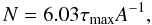 (3)where A = 1.1 × 10⁻¹⁷ cm molec-1 and τmax is the optical depth at the wavelength of the absorption peak (Pontoppidan et al. 2003a).
Since the spectral resolution is low, and since some lines are saturated, it was difficult to estimate the errors in the ice column densities accurately. In the present paper, the column density error was evaluated by simply calculating the error in the absorption area. For CO2, we calculated the absorption area ∫τdν at 4.2−4.3 μm and its error caused by the flux error. Assuming that the absorption area had an error of 11%, and that the CO2 column density was estimated to be 10.0 × 1017 cm-2, for example, the column density error was calculated as 1.1 × 1017 cm-2. For H2O, we estimated the error by calculating the absorption area between 2.8−3.2 μm. If the red wing was much broader than the laboratory spectrum, we estimated the error from the absorption area at 2.8−3.0 μm. For L1527, towards which the H2O band is saturated, we used the wavelength range ~2.8−2.9 μm. The absorption at ~4.7 μm is a combination of the absorptions of CO, XCN, and CO gas (Sect. 4.5). Here, the error is evaluated by calculating the absorption area at 4.65−4.7 μm for CO and 4.57−4.65 μm for XCN. Uncertainties in ice column densities originating from the choice of the convolution function (instrumental line profile or N3 profile) are discussed in Sect. 4.
The derivation of ice column densities described above implicitly assumes a simple geometry: a point light source behind a uniform absorbing material. Edge-on YSOs have more complicated structures. Stellar light scattered by the outflow cavity can be an extended light source (e.g. Tobin et al. 2008), even if it looks like a point source with a PSF of a few arc seconds, and the column density of the absorbing material (envelope and/or disk) also varies spatially. More accurate estimates of the ice column densities requires the radiative transfer calculation of two-dimensional (2D) or three-dimensional (3D) models of envelope and disk structure (Pontoppidan et al. 2005). We compare the observed spectra with existing model calculations and discuss the location of ice in Sect. 5.
4. Results
4.1. Spectrum
Figure 2 shows the derived spectra of our target YSOs. The spectrum of L1041-2 resembles that of L1527, which suggests a similarity in the structure and evolutionary stage of these objects. The spectrum of IRAS 04302, on the other hand, is less reddened than L1527. It might be in a more evolved stage than L1527 and L1041-2.
2MASS J1628137-243139 is very faint and is almost at the faintest limit for which we can derive a spectrum. The spectrum of ASR 41 shows a sharp decline at ~4.5 μm and is noisy at longer wavelengths because of the column pulldown caused by a bright star in the 10′ × 10′ aperture.
HV Tau is a triplet system: HV Tau A and HV Tau B are a binary system with a separation of 0.0728′′ (Simon et al. 1998), and our target edge-on disk, HV Tau C, is separated by ~4′′ from the binary (Woitas & Leinert 1998). Since the FWHM of the AKARI PSF is ~4.3′′ in the NIR and the PSF is not circular, it is difficult to disentangle the HV Tau C spectrum from that of the system. Hence, we integrated the spectral image over an eight-pixel width. The spectrum is dominated by HV Tau A and B at 2.5−4.5 μm, as they are brighter than HV Tau C by 4.22 mag in the K band and >1.71 mag in the L band. At 4.5 μm, on the other hand, the contribution of HV Tau C may not be negligible, because HV Tau C is as bright as the HV Tau AB system in the N band (Woitas & Leinert 1998). HK Tau is also a binary system. The edge-on object, HK Tau B, is a faint binary. Unfortunately, it is impossible to disentangle the spectrum of HK Tau B from the primary, because the two stars almost align in the dispersion direction. It is disappointing that we were unable to discern the spectra of HV Tau C and HK Tau B. The absorption features are, however, still apparent in our spectra. We compare these absorptions with Subaru observations towards the HV Tau C and HK Tau B by Terada et al. (2007) in the following discussion.
The dashed lines in Fig. 2 depict the continuum. While the continuum varies between objects, reflecting their structure and evolutionary stage, we can clearly see absorption bands of H2O (3.05 μm), CO2 (4.27 μm), and CO (4.67 μm) in most of the spectra. The assignment and fitting of each ice band are performed in the following subsections.
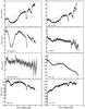 |
Fig. 2 The derived spectra of target YSOs in the NIR (closed circles with error bars). The continuum (dashed line) is determined by the second-order polynomial fitting of the spectrum. |
4.2. H2O ice
Figure 3 shows the spectra normalized by the continuum. The vertical axis is the optical depth of the absorption. Towards L1527 and IRC-L1041-2, the 3.05 μm water band is clearly saturated; the flux at the absorption peak is almost zero (Fig. 2). We fitted the spectra in the range 2.9−3.1 μm with the laboratory spectrum of pure H2O ice at 10 K (Gerakines et al. 1995) (red lines in Fig. 3). We also fitted the observed feature with the pure H2O ice feature at 160 K. The agreement is much worse than for the ice at 10 K, which suggests that the bulk of the observed H2O ice is not annealed.
Interestingly, the profiles fitted at 2.9−3.1 μm (solid lines in Fig. 3) reproduce the shallow hollow at 4.5 μm, which is the O-H combination mode (Boogert et al. 2000). While the 3.05 μm band is saturated, the 4.5 μm band suggests that the H2O column density cannot be significantly larger than we estimated.
Table 2 summarizes the column density of H2O ice derived by fitting the 3.05 μm band. The class 0-I objects L1527, IRAS 04302, and IRC-L1041-2 clearly have much higher water column densities than the other targets, probably because of the larger mass of their circumstellar material and geometrical effects (Sect. 5).
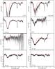 |
Fig. 3 Closed circles with error bars depict the YSO spectrum normalized by the continuum. The absorption feature at 3.05 μm is fitted by the laboratory spectrum of pure H2O ice at 10 K (red line) (see text). |
The observed profiles show a red wing (>3.1 μm), which is often observed in molecular clouds. The shape and depth of the red wing relative to the peak (3.05 μm) vary significantly among objects; it is especially deep towards L1527 and L1041-2. The wing is generally attributed to the scattering by large grains with ice mantles (e.g. Léger et al. 1983). The size of the grains responsible for the red wing is λ/2π ~ 0.5 μm.
ASR 41 has a double-peaked profile at the absorption peak ~3 μm. We reduced each frame of the spectral image to confirm that the double-peaked profile is not caused by noise in a specific frame. The double-peaked profile remained, even if we changed the combination of frames in the stacking. We fitted the profile with (i) the H2O band alone (red line in Fig. 3); and (ii) the H2O band plus an NH3 band (2.98 μm) (blue line in Fig. 3). Although the blue line seems to fit the observed profile slightly better, it results in an unreasonably high column density of NH3 (2 × 1018 cm-2) compared with the H2O column density (7.8 × 1017 cm-2), and the bump at 3.1 μm is not fitted well. While the double-peaked profile seems to be robust, it could still be noise, since the flux at the absorption peak is only 1–2 mJy. We therefore prefer to fit the 3 μm absorption profile with the H2O band alone.
In the polynomial fitting of the HV Tau continuum, we ignored the spectrum at >4.5 μm, since the gradual rise of the spectrum at longer wavelengths may be caused by HV Tau C, while shorter wavelengths are dominated by HV Tau AB. The absorption band at 3 μm is much broader than the laboratory profile. While the red wing may be caused by scattering, the blue wing may be caused by the combination of the spectra of HV Tau A and B. The binary is close enough (~0.07′′) to be considered as a point source in our observation, but the objects have similar brightnesses and different colors (Simon et al. 1998). We tentatively fitted the absorption peak with the laboratory data to derive the water ice column density.
Terada et al. (2007) detected deep H2O absorption towards the edge-on disks of HV Tau C and HK Tau; they concluded that these absorptions originate in the disk ice. If there were no foreground clouds with ice, our spectra should be a combination of the edge-on disk with ice features and bright primaries without absorption. The observed 3 μm absorption of HV Tau is, however, too deep to be accounted for by the disk ice alone; while the flux of HV tau C is 7.75 mJy at K band and 7.14 mJy at L′ band, the 3 μm absorption is as deep as >50 mJy. There must be a contribution of ice absorption in foreground clouds. The H2O column density in Table 2 should be considered as upper limits to the ice in foreground clouds, since we do not distinguish between the disk ice and foreground ice. However, the 3 μm absorption of HK Tau might be due to the disk ice of HK Tau B; the flux of HK Tau B is 15.9 mJy at 2.2 μm and 9.85 mJy at 3.8 μm, while the absorption is ≲ 20 mJy. If we were to assume that the flux of the primary is 200 mJy, subtract it from the spectrum, and fit the 3 μm absorption by the H2O ice feature, the ice column density would be 3 × 1018 cm-2, which is consistent with the value derived by Terada et al. (2007) (3.31 × 1018 cm-2).
Absorption peak, band strength, and column densities of ices towards objects.
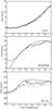 |
Fig. 4 Three-micron spectra of L1527, IRAS 04302, and HK Tau (gray dots with error bars). The thin solid lines in L1527 and IRAS 04302 are the local (3.1–3.7 μm) continua fitted by second order polynomials, while the line in HK Tau is the best-fit absorption of H2O (Fig. 3). Solid and dashed lines depict the upper limits to the pure CH4 ice and pure CH3OH ice absorption depth, respectively. |
4.3. CH band at 3.5 μm
While the long wavelength wing of H2O absorption is generally attributed to scattering by large grains with ice mantles, it might also represent the stretching mode of C-H bond. Among various possible carriers of the C-H bond, CH3OH ice has long been observed via the substructures at 3.47 μm and 3.53 μm (e.g. Grim et al. 1991; Brooke et al. 1996). While the earlier works are mostly restricted to high-mass and intermediate YSOs, Pontoppidan et al. (2003b) identified the 3.5 μm feature towards three low-mass YSOs (out of 40 sources) as CH3OH ice. Boogert et al. (2008) detected the C-O stretching mode of CH3OH at 9.7 μm towards 12 low-mass YSOs (out of 41 sources) using Spitzer. Boogert et al. (2011) detected the 3.53 μm band of CH3OH towards several field stars behind isolated dense cores; the CH3OH/H2O ratio ranges from 5% to 20%. The ratio of CH3OH to H2O column densities varies considerably among objects.
Another possible carrier of the C-H bond is CH4, whose absorption bands at 3.32 μm and 7.67 μm have been detected towards high-mass YSOs (e.g. Lacy et al. 1991; Boogert et al. 2004). Öberg et al. (2008) detected a 7.7 μm absorption feature, which is attributed to CH4, towards 25 sources out of 52 low-mass YSOs. Since CH3OH and CH4 are considered to be the precursors of large organic molecules in hot corinos and WCCC, respectively, it is important to constrain their abundances using the spectrum around 3.5 μm.
Figure 4 shows the spectra of L1527, IRAS 04302, and HK Tau around 3.5 μm. While the spectrum of L1527 is smooth, those of IRAS 04302 and HK Tau contain absorption features. These features, however, do not match either CH3OH or CH4. A potential complication to the identification of, in particular, the CH4 3.32 μm band and to a lesser degree the CH3OH 3.53 μm band, is the possible presence of the 3.3 μm PAH emission feature and the HI Pfδ line at 3.297 μm. We can indeed see an emission feature at 3.3 μm in HK Tau that could be ascribed to the PAH band. In the following, we derive upper limits to the column densities of CH3OH and CH4, keeping in mind that the low spectral resolving power of our spectra may blend adjacent emission and absorption bands.
The thick solid lines in Fig. 4 depict the upper limits on the CH4 absorption depth. We convolved the pure CH4 ice feature at 10 K (Gerakines et al. 1995) with the instrumental line profile (IRAS 04302 and HK Tau) or the N3 profile (for L1527). The upper limits to the CH4 column density are 1.6 × 1019 cm-2 (larger than the H2O column density), 3.1 × 1017 cm-2 (13% relative to H2O), and 1.6 × 1017 cm-2 (76%) towards L1527, IRAS 04302, and HK Tau, respectively. Owing to the low flux, the upper limit towards L1527 is especially high.
The dashed lines show the upper limits to the CH3OH absorption depths, using a laboratory spectrum for pure CH3OH at 10 K (Gerakines et al. 1995), convolved with the instrumental line profile. While the 3.53 μm feature is common among pure CH3OH ice and mixed ice (H2O+CH3OH), the shape and depth of the 3.4 μm feature depend on the composition of the mixture (e.g. Pontoppidan et al. 2003b). Hence, we derived upper limits to the CH3OH column density of the 3.53 μm feature. The upper limits to the CH3OH column densities are 1.2 × 1018 cm-2 (26% relative to H2O), 1.0 × 1018 cm-2 (42%), and 3.1 × 1017 cm-2 (larger than the H2O column) towards L1527, IRAS 04302, and HK Tau, respectively.
4.4. HDO ice
In some objects, such as IRAS 04302, we can see absorption around 4.1 μm, where the OD stretching mode of HDO is observed in the laboratory (Dartois et al. 2003). Since the detection of HDO ice is very rare (Teixeira et al. 1999) and has not been confidently confirmed, we checked the response function carefully and confirmed that the ~4.1 μm feature is not caused by an artifact in the response function. Figure 5 shows the spectra of this wavelength region towards L1527, IRC-L1041-2, IRAS 04302, and HV Tau, which are fitted with a model of the amorphous HDO feature at 10 K: a Gaussian profile peaking at 4.07 μm with a FWHM of 0.2 μm (solid lines). The spectrum of L1527 is not fitted well with this Gaussian; the absorption has a peak at longer wavelength (~4.13 μm) and a narrower band width, which resembles an annealed, rather than an amorphous, HDO feature (Dartois et al. 2003). We fitted the L1527 spectrum with a Gaussian peaking at 4.13 μm and FWHM of 0.1 μm (dashed line in Fig. 5).
Although IRAS 04302 has the deepest and smoothest absorption around 4.1 μm, this result should be taken with caution. The spectrum also shows a broad absorption at 4.5−4.6 μm, which cannot be fitted well by the absorptions of CO and XCN (see Sect. 4.6). These two absorptions (4.1 μm and 4.5−4.6 μm) could be related; there could be an alternative explanation, rather than HDO, CO, and XCN. The features themselves are, however, robust. We have two independent data sets of IRAS 04302, and the two broad absorptions appear in both data sets.
We integrated the fitted spectra to derive the column density of HDO (Table 2). The band strength was assumed to be 4.3 × 10⁻¹⁷ cm molecule-1 (Dartois et al. 2003). Considering the small bumps and hollows that deviate from the HDO feature and the above discussion of IRAS 04302 spectrum, the HDO column densities should be interpreted with caution. However, at face value, the HDO/H2O ratio ranges from 2% (L1527) to 22% (IRAS 04302). Except in the case of L1527, the ratios are much higher than those obtained in the previous observations and theoretical works: HDO/H2O ≤ 3% (Dartois et al. 2003; Parise et al. 2003, 2005; Aikawa et al. 2005).
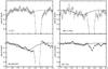 |
Fig. 5 Spectra around the HDO absorption band. The solid line is the Gaussian with FWHM of 0.2 μm approximating the amorphous HDO ice feature, while the dashed line approximates the annealed HDO feature. |
4.5. CO2 ice
The CO2 band at 4.27 μm is clearly detected towards our targets, except ASR41 and 2MASS J1628137. To subtract the H2O band at 4.5 μm, we divide the normalized spectrum by the best-fit H2O profile (red line in Fig. 3). The absorption at 4.27 μm is then fitted by the laboratory CO2 profile convolved by the instrumental line profile (N3 profile for L1527) (solid line in Fig. 6). To illustrate how the profile is broadened by the instrumental line profile, the laboratory profile before convolution is shown in the panel of IRAS 04302 with the dashed line. While we adopted the pure CO2 profile measured by Gerakines et al. (1995) at 10 K, the actual shape of the CO2 profile depends on various factors, such as its mixing with other ice species, grain shape, and annealing (Ehrenfreund et al. 1997; van Broekhuizen et al. 2006). We tried to fit the absorption bands with those of mixed ices of CO2:CO = 1:1 at 15 K, and H2O:CO2 = 100:14 at 10 K, but the fits were worse than the pure CO2 ice of 10 K. Although the observed profile might be better fitted by other mixtures and temperatures, we do not pursue this fitting, because the spectral resolution of the IRC is not high enough.
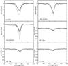 |
Fig. 6 Spectra fitted by the convolved laboratory spectrum of CO2 ice (solid line). The dashed lines depict the CO2 feature before convolution. In the panel of L1527, the 4.38 μm feature is fitted by the convolved laboratory spectrum of 13CO2 (thin solid line). |
In regions close to the YSO, CO2 sublimates at ~70 K. We note that CO2 gas has absorption lines in almost the same wavelength range as CO2 ice. Although the observed feature might be a combination of CO2 ice and gaseous CO2, the low spectral resolving power makes it difficult to distinguish between gas and ice. We tried to fit the observed feature with CO2 gas of constant temperature (20 K, 70 K, and 150 K), but the observed features are better fitted by the pure CO2 ice.
We obtained the CO2 ice column densities listed in Table 2. The errors listed in Table 2 were derived from the errors in the absorption area. For class 0-I sources, the convolution function (the instrumental line profile or the N3 profile) might add errors to the column densities. For IRC-L1041, if we were to adopt the N3 profile, the CO2 column density should be larger by ~30% than listed in Table 2; the wing region is reproduced better, but the agreement in the peak region is worse than in Fig. 6. For IRAS 04302, convolution with its N3 profile makes the absorption peak more flat and thus in closer agreement with the observation, while the CO2 column density is little changed.
We also detected CO2 absorption towards HV Tau and HK Tau. The absorption could, at least partially, originate in the circumstellar disks. The H2O absorption towards HK Tau could originate solely in the disk of HK Tau B (Sect. 4.2). If so, the detected CO2 ice towards HK Tau should also be in the edge-on disk, since it is unlikely that the foreground clouds contain CO2 but no H2O. The CO2 absorptions of HK Tau and HV Tau are, however, deeper than 10 mJy, while the fluxes of HV Tau C and HK Tau B seem to reach a maximum in the K band, and are smaller than 10 mJy at 3.8 μm and probably at longer wavelength (Sect. 4.2). Hence, we derived the CO2 ice column density by normalizing the spectrum with the continuum plotted in Fig. 2, as if the CO2 ice originates in the foreground clouds of the primary.
The relation between column densities of CO2 ice and H2O ice is plotted in Fig. 7. Our class 0-I stars show similar CO2/H2O ratios to those observed by Pontoppidan et al. (2008) towards embedded low-mass YSOs using SST. Towards HV Tau, HK Tau, and UY Aur, on the other hand, the column densities of H2O ice and CO2 ice are much lower than observed by Pontoppidan et al. (2008), assuming that the detected absorption features all originate in the foreground clouds. The CO2/H2O ratios toward these class II objects, however, agree with the range of ratios for low-mass YSOs from Pontoppidan et al. (2008).
We note that the 13CO2 band at 4.38 μm is apparent in the spectra of L1527 and IRC-L1041-2. The laboratory CO2 profile used to fit the 4.27 μm feature contains 13CO2 with the terrestrial ratio 12C/13C = 89. In L1527, we fitted the 4.38 μm feature (thin solid line in Fig. 6) with the laboratory spectrum. The absorption area (∫τdν) of the thin solid line is about two times larger than that of the thick solid line, indicating that the 12CO2/13CO2 ratio could be lower than the terrestrial value. However, when considering the S/N, we found that the observed 4.38 μm feature is consistent with the thick solid line in Fig. 6, which fits the 4.27 μm feature; the terrestrial ratio 12C/13C = 89 are not significantly inconsistent with our observational data.
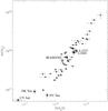 |
Fig. 7 The relation between column densities of H2O ice and CO2 ice towards our targets (crosses) plotted over Fig. 6 of Pontoppidan et al. (2008); the diamonds are low-mass stars observed by Pontoppidan et al. (2008), and the open triangles are the background stars from Whittet et al. (2007) and Knez et al. (2005). |
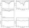 |
Fig. 8 The spectra around the CO ice absorption band fitted by a combination (thick solid line) of CO gas (dashed line), XCN feature (dotted line), and CO ice on the CDE grain model (thin solid line). The dot-dashed line in the panel of L1527 depicts the CO ice feature before the convolution with the N3 profile. |
4.6. CO and XCN
We found that CO ice has an absorption band at 4.67 μm. Figure 8 shows the spectra around this wavelength towards L1527 and IRC-L1041-2, IRAS 04302, HK Tau, and UY Aur.
Both L1527 and IRC-L1041-2 clearly have double-peaked profiles. The blue peak coincides with the XCN band, and the red peak matches the CO ice band. Although the double peak can be reproduced by combining XCN and CO ice, the observed features have an additional component at ~4.7–4.75 μm. We assume that this corresponds to CO gas because, owing to the low sublimation temperature (~20 K), CO can be more easily sublimated and excited near the protostar than CO2. With the low spectral resolution of IRC, gaseous CO vibrational bands cannot be observed as lines but become a broad double-peaked (P branch and R branch) feature. It is thus difficult to derive the CO gas column density from our data. However, it is important to subtract the CO gas absorption, since the R branch of the CO gas feature coincides with the XCN feature. The distance between the P branch and R branch increases with temperature. We fitted the absorption at 4.7−4.75 μm with a CO gas profile at 70 K that had been smoothed to the low spectral resolution (dashed lines in Fig. 8).
After the subtraction of CO gas absorption, we fitted the XCN feature, assuming a Gaussian peaking at 4.62 μm with FWHM of 29.1 cm-1 (Gibb et al. 2004) (dotted lines in Fig. 8), and the CO ice feature using the CDE grain model of Ehrenfreund et al. (1997) (thin solid lines in Fig. 8). The dot-dashed line in Fig. 8 depicts the laboratory spectrum before convolution, and the thick solid lines in Fig. 8 shows the sum of the three fitted components.
The absorption feature around 4.67 μm is also observed towards HK Tau and UY Aur, but the feature does not peak at 4.67 μm. We tentatively assigned the absorption to gaseous CO at 70 K and 150 K for HK Tau and UY Aur, respectively (dashed lines in Fig. 8).
Table 2 lists the estimated column densities of CO ice. The correlation between the column densities of CO ice and H2O ice is plotted in Fig. 9 over the correlation towards field stars of Whittet et al. (2007). The gray square depicts the ice column density ratio towards class I protostar Elias 29 (Boogert 2000). Our targets show higher CO/H2O ratios than Elias 29, probably because our targets are edge-on objects. IRAS 04302 shows a lower ratio of CO/H2O than field stars, indicating that its circumstellar material is warmer and/or less dense than typical molecular cloud gas.
Assuming that the XCN is OCN−, we adopt the band strength of A(XCN) = 5 × 10-17 cm mol-1, and estimate the OCN− column density to be (0.5−2.5) × 1017 cm-2 towards class 0-I objects (Table 2). The column density ratio of OCN−/H2O ranges from 2.2% (IRAS 04302) to 6.4% (L1041-2). Weintraub et al. (1994) detected the XCN feature towards a T Tauri star RNO 91 and derived an upper limit to the XCN/H2O ratio of ≲ 9%. More recent works, on the other hand, have derived much lower XCN/H2O ratio towards low-mass YSOs. van Broekhuizen et al. (2005) observed low-mass YSOs with VLT; the column density ratio of OCN−/H2O is ≤ 0.85%. Although CO gas can contribute to the absorption at ~4.62 μm in our spectra, its contribution is subtracted by referring to the absorption at 4.7−4.75 μm. In laboratory experiments, thermal or UV processing of N-bearing ice produces OCN− (Schutte & Greenberg 1997). Since our targets are edge-on objects, our lines of sight may preferentially trace the surface region of the disks (or the dense torus region of the envelope) where OCN− is produced by UV irradiation. The OCN− column densities towards IRC-L1041 and IRAS 04302, however, should be taken with caution, since there is residual absorption in the 4.5−4.6 μm region (Fig. 8). If there are other unknown carriers at these wavelengths, the estimated OCN− column densities are upper limits.
Both L1527 and IRC-L1041-2 show weak absorption at ~4.78 μm. Although it is close to the peak of 13CO ice feature, the observed peak is at a slightly shorter wavelength than that of 13CO.
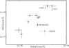 |
Fig. 9 The relation between the column densities of H2O ice and CO ice towards our targets (square). The crosses are ice columns towards field stars observed by Whittet et al. (2007). The gray square depicts the ice column density towards the low-mass class I protostar Elias29 (Boogert et al. 2000). |
4.7. OCS
IRC-L1041-2 has an absorption feature at ~4.9 μm. This coincides with the OCS ice band, which can be approximated by a Gaussian peaking at 4.91 μm with a FWHM of 19.6 cm-1 (Gibb et al. 2004; Palumbo et al. 1997; Hudgins et al. 1993). Although the feature is at the edge of the observable wavelength range of the IRC and should be treated with caution, it does not disappear even if we change the combination of frames to be stacked. We fitted the spectrum with a Gaussian (Fig. 10). Assuming a band strength of 1.7 × 10⁻¹⁸ cm molecule-1 (Hudgins et al. 1993), the OCS column density towards IRC-L1041-2 is 6.2 × 1016 cm-2. If the abundance of H2O ice relative to hydrogen nuclei is 1 × 10⁻⁴, the hydrogen column density in the line of sight is 3.9 × 1022 cm-2, and the relative abundance of OCS ice to hydrogen is 1.6 × 10⁻⁶, which is much higher than the abundance of gaseous OCS, 1 × 10⁻⁹, observed towards TMC-1 (Irvine et al. 1987).
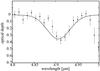 |
Fig. 10 Spectrum of IRC-L1041-2 at 4.9 μm. The solid line is a Gaussian with FWHM 19.6 cm-1 approximating the OCS absorption feature. |
5. Discussion
5.1. Location of the Ice
Young stellar objects have a complicated structure: a protostar, circumstellar disk, envelope, and outflow cavity. Furthermore, some objects might be accompanied by either ambient or foreground clouds. In our observation of edge-on YSOs, the light source is not necessarily the central star. The NIR light of 3−5 μm can originate from, for example, a wall of the outflow cavity that scatters the stellar light. The light source can thus be spatially extended relative to the projected spatial scale of ice abundance structures, even if it looks like a point source (e.g. Tobin et al. 2008, 2010), and the absorbing material in the envelope and/or disk also has non-uniform spatial distributions. Although the radiative transfer modeling of such an envelope and disk system is beyond the scope of the present work, it is important to discuss the location of ice in our targets.
5.1.1. Class 0-I objects
Among the three class 0-I objects, L1527 is the most well-studied. Its bolometric temperature is less than 70 K, suggesting that the object is deeply embedded in dense gas (Furlan et al. 2008). Tobin et al. (2008) constructed an axisymmetric model of the envelope and disk with an outflow cavity referring to the SST images and SED of the object. According to the model, the “central object” we see in the N3 image is scattered light from the “inner cavity” with a size of ~100 AU. If so, the ice absorption bands in our spectrum most likely originate in the envelope rather than the disk. The envelope density ranges from about 108 cm-3 to 105 cm-3 at ~100 AU to 15 000 AU. The integrated envelope column density in the line of sight is ~1 g cm-2, which corresponds to a hydrogen column density of NH ~ 4 × 1023 cm-2. This would, however, be an overestimate, because the envelope structure is not axisymmetric in reality.
Owing to the similarity of the continuum spectra, we expect L1041 and L1527 to have a similar physical structure. Varying depths of ice absorptions among these objects would thus probe the difference in the ice composition in the envelope.
The SED modeling of the YSOs suggests that the envelope of IRAS 04302 is slightly less dense than L1527 (Furlan et al. 2008). We found smaller column densities of ices and lower CO/CO2 ice ratios towards IRAS 04302 than L1527, which also indicates that IRAS 04302 is more evolved and has a less massive envelope.
Although our observations probe ice in envelopes rather than disks, the envelope material along our lines of sight (perpendicular to the rotation axis and outflow) is more likely to end up in the forming disks than be dissipated in the clouds. The high CO/CO2 ice ratio indicates that the majority of gases in the lines of sight are still dense and cold. The CO2/H2O ratio towards our objects is similar to the ratio observed by Pontoppidan et al. (2008), who observed low-mass YSOs with various inclinations; the CO2/H2O ratio does not seem to vary with the inclination angle.
The CO gas absorption and deep absorption feature of OCN−, on the other hand, would originate in the warm (T ≥ 20 K) and irradiated region near the protostar. However, other signs of heating by the protostar, such as crystalline feature of H2O ice (Schegerer & Wolf 2010) and CO2 gas, are not found in our data. We may need higher spatial resolution and spectral resolution to detect these features.
5.1.2. Edge-on class II objects: ASR41 and 2MASS J1628137
We estimated the H2O ice column density from our observations to be 7.8 × 1017 cm-2 towards ASR41 and 6.7 × 1017 cm-2 towards 2MASS J1628137. These values are apparently much lower than we expect from the theoretical prediction of high H2O ice abundance n(H2O)/nH ~ 10-4 in the disk midplane. The shallow absorption is, however, caused by a geometric effect. Pontoppidan et al. (2005) predicts that the 3 μm water band is the deepest for the disk inclination of ~70° and becomes shallower for higher inclination angles. If the inclination angle is ≥72°, the optical depth of the band is predicted to be ~0.6, which is comparable to our observation of ASR41. Since the light source (scattered stellar light) is more extended than the absorbing material, Eq. (2) underestimates the ice column density towards edge-on disks.
Possible contributions to the observed ice column densities from foreground clouds should also be considered. In the Taurus molecular cloud, the average H2O abundance is about 8.6 × 10⁻⁵ relative to hydrogen nuclei at Av ≥ 3 mag (Whittet et al. 1993; Chair et al. 2011). The H2O ice is not detected at lower Av, which indicates that H2O ice is easily destroyed by photolysis or photodesorption near the cloud surface. Hodapp et al. (2004) estimated that the density and size of the molecular cloud around ASR 41 are 2.0 × 10⁻²⁰ g cm-3 and 104 AU, which corresponds to AV ~ 1 mag. Although the relative abundance and the threshold Av varies from cloud to cloud, the column density of the foreground gas towards ASR41, Av ~ 1 mag, is too small to contribute significantly to the H2O ice absorption band. Therefore, the observed H2O ice most likely originates in the disk around ASR41.
The foreground visual extinction towards 2MASSJ 1628137, on the other hand, is estimated to be AV = 2.1 ± 2.6 mag (Grosso et al. 2003 ). Assuming that the H2O ice abundance and threshold Av are the same as in Taurus, the upper limit of the foreground H2O ice column density is ~2 × 1017 cm-2, which is smaller than the observed H2O ice column (6.7 × 1017 cm-2). Hence, we conclude that most or all of the H2O ice observed towards 2MASSJ 1628137 originates in the disk.
5.1.3. Other class II objects
HV Tau and HK Tau are multiple systems. As the separation between the multiple components in these systems is smaller than the size of our PSF in the NIR, we cannot extract the spectra of the faint edge-on objects. Terada et al. (2007) observed 2−2.5 μm and 3−4 μm spectra of these edge-on objects using Subaru and detected deep water absorption (τ ~ 1−1.5). The continuum flux of HV Tau C is ~7.75 mJy at 2.2 μm and ~7.14 mJy at 3.8 μm, while the flux of HK Tau B is ~15.9 mJy at 2.2 μm and ~9.85 mJy at 3.8 μm. Apparently, our spectra are dominated by the bright primaries. Both H2O and CO2 ice absorptions towards HV Tau should originate in both the disk and foreground clouds, since the depths of the absorption bands are larger than the continuum flux of the HV Tau C. Towards HK Tau, the depth of the H2O absorption is comparable to the continuum flux of HK Tau B; if the H2O absorption originates in the disk around HK Tau B, the H2O ice column density is ~3 × 1018 cm-2, which is comparable to the value obtained by Terada et al. (2007). The CO2 absorption, on the other hand, is deeper than the continuum flux of HK Tau B, and thus should originate at least partially in the foreground clouds. We also detected shallow H2O ice bands towards UY Aur, which again originate in the foreground component, since the inclination of the disk is ~42 degrees.
If the H2O absorptions towards HV Tau and HK Tau originated in the foreground clouds, the estimated H2O ice column densities would be smaller than the H2O ice column densities in the edge-on disks obtained by Terada et al. (2007) by about an order of magnitude; the H2O ice column density would be 3.31 × 1018 cm-2 for HK Tau B, and (2.69−4.20) × 1018 cm-2 for HV Tau C. Our observations thus support the argument of Terada et al. (2007) that the disk component overwhelms the foreground component towards HK Tau B and HV Tau C.
6. Conclusions
We have observed ice absorption bands at 2.5−5 μm towards eight low-mass YSOs: three class 0-I protostellar cores with edge-on geometry, two edge-on class II objects, two multiple systems with edge-on class II, and one not-edge-on class II object.
Towards the class 0-I objects, L1527, IRC-L1041-2, and IRAS 04302, we have detected abundant H2O, CO2, and CO ice in the envelope. The column density ratio of CO2 to H2O ice is 21−28%, which coincides with the ratio observed by SST towards YSOs with various inclinations. The weak absorption at ~4.1 μm can be fitted by HDO ice; the HDO/H2O ratio ranges from 2% to 22%. The absorption in the vicinity of the CO band (4.76 μm) is double-peaked and fitted by combining CO ice, OCN−, and CO gas. The large column density of CO ice suggests that the envelope is still very dense and cold, while OCN− and CO gas features would originate in the region close to the protostar. The column density of OCN− is as high as 2−6% relative to H2O, which is much higher than previous observations. Our lines of sight (high inclinations from the rotation axis) may preferentially trace the regions with high UV irradiation, such as the surface of a forming disk and/or torus envelope.
The spectrum of IRAS 04302 includes the 3.5 μm absorption band, but the feature does not match either CH3OH or CH4. An OCS absorption band is tentatively detected towards IRC-L1041-2.
Towards the edge-on class II objects, ASR41 and 2MASS J1628137-243139, we have detected the H2O band. The low optical depth of the water feature is due to geometrical effects (Pontoppidan et al. 2005). The detected water ice mainly originates in the disk.
Both HK Tau B and HV Tau C are edge-on class II objects in multiple systems. In our spectra, which are dominated by the primaries, we have detected the absorption of H2O ice and CO2 ice. Ices in both the edge-on disks and foreground clouds would contribute to the absorption, although H2O absorption towards HK Tau could originate solely in the disk. Even if the observed features are due to the foreground clouds, the H2O ice column densities in the clouds are much smaller than those observed towards HK Tau B and HV Tau C with Subaru (Terada et al. 2007), which confirms that the ice columns of the latter must originate in disks. The foreground H2O ice and CO2 ice are also detected towards UY Aur, which is not an edge-on system. We have tentatively detected CO gas towards HK Tau and UY Aur.
Acknowledgments
We would like to thank the project members of AKARI and AFSAS team for their help with the observation. We are grateful to Dr. D. Heinzeller for providing models of gas absorption features and to Prof. Whittet for his permission to use the CO/H2O plot from Whittet et al. (2007). We would like to thank the anonymous referee for helpful comments that helped to improve the manuscript. This work was supported by a grant-in-aid for scientific research (19740103, 23540266, 23103004).
References
- Aikawa, Y., Herbst, E., Roberts, H., & Caselli, P. 2005, ApJ, 620, 330 [NASA ADS] [CrossRef] [Google Scholar]
- Aikawa, Y., Wakelam, V., Garrod, T. R., & Herbst, E. 2008, ApJ, 674, 984 [NASA ADS] [CrossRef] [Google Scholar]
- André, P., Ward-Thompson, D., & Barsony, M. 2000, Protostars and Planets IV, 59 [Google Scholar]
- Boogert, A. C. A., Tielens, A. G. G. M., Ceccarelli, C., et al. 2000, A&A, 360, 683 [NASA ADS] [Google Scholar]
- Boogert, A. C. A., Blake, G. A., & Tielens, A. G. G. M. 2002, ApJ, 577, 271 [NASA ADS] [CrossRef] [Google Scholar]
- Boogert, A. C. A., Blake, G. A., & Öberg, K. 2004, ApJ, 615, 344 [NASA ADS] [CrossRef] [Google Scholar]
- Boogert, A. C. A., Pontoppidan, K. M., Knez, C., et al. 2008, ApJ, 678, 985 [NASA ADS] [CrossRef] [Google Scholar]
- Boogert, A. C. A., Huard, T. L., Cook, A. M., et al. 2011, ApJ, 729, 92 [NASA ADS] [CrossRef] [Google Scholar]
- Brooke, T. Y., Sellgren, K., & Smith, R. G. 1996, ApJ, 459, 2009 [Google Scholar]
- Chair, J. E., Pendleton, Y. J., Allamandola, L. J., et al. 2011, ApJ, 731, 9 [NASA ADS] [CrossRef] [Google Scholar]
- Dartois, E., Thi, W. F., Geballe, T. R., et al. 2003, A&A, 399, 1020 [Google Scholar]
- Ehrenfreund, P., Boogert, A. C. A., Gerakines, P. A., Tielens, A. G. G. M., & van Dishoeck, E. F. 1997, A&A, 328, 649 [NASA ADS] [Google Scholar]
- Furlan, E., McClure, M., Calvet, N., et al. 2008, ApJS, 176, 184 [NASA ADS] [CrossRef] [Google Scholar]
- Geers, V. C., van Dishoeck, E. F., Visser, R., et al. 2007, A&A, 476, 279 [NASA ADS] [CrossRef] [EDP Sciences] [Google Scholar]
- Gerakines, P. A., Schutte, W. A., Greenberg, J. M., & van Dishoeck, E. F. 1995, A&A, 296, 810 [NASA ADS] [Google Scholar]
- Gerakines, P. A., Schutte, W. A., & Ehrenfreund, P. 1996, A&A, 312, 289 [NASA ADS] [Google Scholar]
- Gibb, E. L., Whittet, D. C. B., Schutte, W. A., et al. 2000, ApJ, 536, 347 [NASA ADS] [CrossRef] [Google Scholar]
- Gibb, E. L., Whittet, D. C. B., Boogert, A. C. A., & Tielens, A. G. G. M. 2004, ApJS, 151, 35 [NASA ADS] [CrossRef] [PubMed] [Google Scholar]
- Grim, R. J. A., Baas, F., Geballe, T. R., Greenberg, G. M., & Schutte, W. 1991, A&A, 243, 473 [NASA ADS] [Google Scholar]
- Grosso, N., Alves, J., Wood, K., et al. 2003, ApJ, 586, 296 [NASA ADS] [CrossRef] [Google Scholar]
- Hioki, T., Itoh, Y., Oasa, Y., et al. 2007, ApJ, 134, 880 [Google Scholar]
- Hodapp, K. W., Walker, C. H., Reipurth, B., et al. 2004, ApJ, 601, L79 [NASA ADS] [CrossRef] [Google Scholar]
- Honda, M., Inoue, A. K., Fukagawa, M., et al. ApJ, 690, L110 [Google Scholar]
- Hudgins, D. M., Sandford, S. A., Allamandola, L. J., & Tielens, A. G. G. M. 1993, ApJS, 86, 713 [NASA ADS] [CrossRef] [Google Scholar]
- Irvine, W. M., Goldsmith, P. F., & Hjalmarson, A. 1987, in Interstellar processes, ed. D. J. Hollenbach, & H. A. Jr. Thronson, 561 [Google Scholar]
- Knez, C., Boogert, A. C. A., Pontoppidan, K. M., et al. 2005, ApJ, 635, L145 [NASA ADS] [CrossRef] [Google Scholar]
- Lacy, J. H., Carr, J. S., Evans, N. J.II, et al. 1991, ApJ, 376, 556 [NASA ADS] [CrossRef] [Google Scholar]
- Léger, A., Gauthier, S., Defourneau, D., & Rouan, D. 1983, A&A, 117, 164 [NASA ADS] [Google Scholar]
- Monin, J.-L., & Bouvier, J. 2000, A&A, 356, L75 [NASA ADS] [Google Scholar]
- Murakami, H., Baba, H., Barthel, P., et al. 2007, PASJ, 59, 369 [Google Scholar]
- Murakawa, K., Tamura, M., & Nagata, T. 2000, ApJS, 128, 603 [NASA ADS] [CrossRef] [Google Scholar]
- Öberg, K. I., Boogert, A. C. A., Pontoppidan, K. M., et al. 2008, ApJ, 678, 1032 [NASA ADS] [CrossRef] [Google Scholar]
- Ohyama, Y., Onaka, T., Matsuhara, H., et al. 2007, PASJ, 59, 411 [NASA ADS] [Google Scholar]
- Onaka, T., Matsuhara, H., Wada, T., et al. 2007, PASJ, 59, 401 [NASA ADS] [Google Scholar]
- Palumbo, M. E., Geballe, T. R., & Tielens, A. G. G. M. 1997, ApJ, 479, 839 [NASA ADS] [CrossRef] [Google Scholar]
- Parise, B., Simon, T., Caux, E., et al. 2003, A&A, 410, 897 [NASA ADS] [CrossRef] [EDP Sciences] [Google Scholar]
- Parise, B., Caux, E., Castets, A., et al. 2005, A&A, 431, 547 [NASA ADS] [CrossRef] [EDP Sciences] [Google Scholar]
- Pontoppidan, K. M., & Dullemond, C. P. 2005, A&A, 435, 595 [NASA ADS] [CrossRef] [EDP Sciences] [Google Scholar]
- Pontoppidan, K. M., Fraser, H. J., Dartois, E., et al. 2003a, A&A, 408, 981 [NASA ADS] [CrossRef] [EDP Sciences] [Google Scholar]
- Pontoppidan, K. M., Dartois, E., van Dishoeck, E. F., Thi, W.-F., & d’Hendecourt, L. 2003b, A&A, 404, L17 [NASA ADS] [CrossRef] [EDP Sciences] [Google Scholar]
- Pontoppidan, K. M., Boogert, A. C. C., Fraser, H. J., et al. 2008, ApJ, 678, 1005 [NASA ADS] [CrossRef] [Google Scholar]
- Sakai, N., Sakai, T., Hirota, T., & Yamamoto, S. 2008, ApJ, 672, 371 [NASA ADS] [CrossRef] [Google Scholar]
- Sakon, I., Onaka, T., Wada, T., et al. 2007, PASJ, 59, 483 [NASA ADS] [CrossRef] [Google Scholar]
- Schutte, W. A., & Greenberg, J. M. 1997, A&A, 317, L43 [NASA ADS] [Google Scholar]
- Schegerer, A. A., & Wolf, S. 2010, A&A, 517, A87 [NASA ADS] [CrossRef] [EDP Sciences] [Google Scholar]
- Simon, M., Holfeltz, S. T., & Taff, L. G. 1998, ApJ, 469, 890 [Google Scholar]
- Smith, R. G., Sellgren, K., & Tokunaga, A. T. 1989, ApJ, 344, 413 [NASA ADS] [CrossRef] [Google Scholar]
- Stapelfeldt, K. R., Krist, J. E., Menard, F., et al. 1998, ApJ, 502, L65 [NASA ADS] [CrossRef] [Google Scholar]
- Terada, H., Tokunaga, A. T., Kobayashi, N., et al. 2007, ApJ, 667, 303 [NASA ADS] [CrossRef] [Google Scholar]
- Teixeira, T. C., & Emerson, J. P. 1999, A&A, 351, 303 [NASA ADS] [Google Scholar]
- Thi, W. F., Pontoppidan, K. M., van Dishoeck, E. F., Dartois, E. & d’Hendecourt, L. 2002, A&A, 394, L27 [NASA ADS] [CrossRef] [EDP Sciences] [Google Scholar]
- Tobin, J. J., Hartmann, L., Calvet, N., & D’Alessio, P. 2008, ApJ, 679, 1364 [NASA ADS] [CrossRef] [Google Scholar]
- Tobin, J. J., Hartmann, L., Looney, L. W., & Chiang, H.-F. 2010, ApJ, 712, 1010 [NASA ADS] [CrossRef] [Google Scholar]
- van Broekhuizen, F. A., Keane, J. V., & Schutte, W. A. 2004, A&A, 415, 425 [NASA ADS] [CrossRef] [EDP Sciences] [Google Scholar]
- van Broekhuizen, F. A., Pontoppidan, K. M., Fraser, H. J., & van Dishoeck, E. F. 2005, A&A, 441, 249 [NASA ADS] [CrossRef] [EDP Sciences] [Google Scholar]
- van Broekhuizen, F. A., Groot, I. M. N., Fraser, H. J., van Dishoeck, E. F., & Schlemmer, S. 2006, A&A, 451, 273 [NASA ADS] [CrossRef] [EDP Sciences] [Google Scholar]
- van Dishoeck, E. F., Helmich, F. P., de Graauw, Th., et al. 1996, A&A, 315, L349 [NASA ADS] [Google Scholar]
- Visser, R., van Dishoeck, E. F., Doty, S. D., & Dullemond, C. P. 2009, A&A, 495, 881 [NASA ADS] [CrossRef] [EDP Sciences] [Google Scholar]
- Weintraub, D. A., Tegler, S. C., Kastner, J. H., & Rettig, T. 1994, ApJ, 423, 674 [NASA ADS] [CrossRef] [Google Scholar]
- Whittet, D. C. B. 1993, Dust and Chemistry in Astronomy (Bristol and Philadelphia: Institute of Physics Publishing), 9 [Google Scholar]
- Whittet, D. C. B., Gerakines, P. A., Tielens, A. G. G. M., et al. 1998, ApJ, 498, 159 [Google Scholar]
- Whittet, D. C. B., Shenoy, S. S., Bergin, E. A., et al. 2007, ApJ, 655, 332 [NASA ADS] [CrossRef] [Google Scholar]
- Woitas, J., & Leinert, Ch. 1998, A&A, 338, 122 [NASA ADS] [Google Scholar]
- Wolf, S., Padgett, D., & Stapelfeldt, K. R. 2003, ApJ, 588, 373 [NASA ADS] [CrossRef] [Google Scholar]
- Zasowski, G., Kemper, F., Watson, D. M., et al. 2009, ApJ, 694, 459 [NASA ADS] [CrossRef] [Google Scholar]
All Tables
All Figures
|
Fig. 1 a) Images of our targets taken by AKARI with the N3 filter (2.7−3.8 μm). The stellar light is dispersed from right (short wavelength) to left (long wavelength). The FOV is 1′ × 1′. The coordinate at the center of the FOV is listed in Table 1. Images of IRC-L1041-2 and 2MASS J1628137-243139 are damaged by cosmic rays, while images of HV Tau, HK Tau, ASR41, and UY Aur are affected by saturation and column pull down. b) Spectral images of 1527 and IRAS 04302. |
| In the text | |
|
Fig. 2 The derived spectra of target YSOs in the NIR (closed circles with error bars). The continuum (dashed line) is determined by the second-order polynomial fitting of the spectrum. |
| In the text | |
|
Fig. 3 Closed circles with error bars depict the YSO spectrum normalized by the continuum. The absorption feature at 3.05 μm is fitted by the laboratory spectrum of pure H2O ice at 10 K (red line) (see text). |
| In the text | |
|
Fig. 4 Three-micron spectra of L1527, IRAS 04302, and HK Tau (gray dots with error bars). The thin solid lines in L1527 and IRAS 04302 are the local (3.1–3.7 μm) continua fitted by second order polynomials, while the line in HK Tau is the best-fit absorption of H2O (Fig. 3). Solid and dashed lines depict the upper limits to the pure CH4 ice and pure CH3OH ice absorption depth, respectively. |
| In the text | |
|
Fig. 5 Spectra around the HDO absorption band. The solid line is the Gaussian with FWHM of 0.2 μm approximating the amorphous HDO ice feature, while the dashed line approximates the annealed HDO feature. |
| In the text | |
|
Fig. 6 Spectra fitted by the convolved laboratory spectrum of CO2 ice (solid line). The dashed lines depict the CO2 feature before convolution. In the panel of L1527, the 4.38 μm feature is fitted by the convolved laboratory spectrum of 13CO2 (thin solid line). |
| In the text | |
|
Fig. 7 The relation between column densities of H2O ice and CO2 ice towards our targets (crosses) plotted over Fig. 6 of Pontoppidan et al. (2008); the diamonds are low-mass stars observed by Pontoppidan et al. (2008), and the open triangles are the background stars from Whittet et al. (2007) and Knez et al. (2005). |
| In the text | |
|
Fig. 8 The spectra around the CO ice absorption band fitted by a combination (thick solid line) of CO gas (dashed line), XCN feature (dotted line), and CO ice on the CDE grain model (thin solid line). The dot-dashed line in the panel of L1527 depicts the CO ice feature before the convolution with the N3 profile. |
| In the text | |
|
Fig. 9 The relation between the column densities of H2O ice and CO ice towards our targets (square). The crosses are ice columns towards field stars observed by Whittet et al. (2007). The gray square depicts the ice column density towards the low-mass class I protostar Elias29 (Boogert et al. 2000). |
| In the text | |
|
Fig. 10 Spectrum of IRC-L1041-2 at 4.9 μm. The solid line is a Gaussian with FWHM 19.6 cm-1 approximating the OCS absorption feature. |
| In the text | |
Current usage metrics show cumulative count of Article Views (full-text article views including HTML views, PDF and ePub downloads, according to the available data) and Abstracts Views on Vision4Press platform.
Data correspond to usage on the plateform after 2015. The current usage metrics is available 48-96 hours after online publication and is updated daily on week days.
Initial download of the metrics may take a while.