| Issue |
A&A
Volume 537, January 2012
|
|
|---|---|---|
| Article Number | A120 | |
| Number of page(s) | 22 | |
| Section | Stellar structure and evolution | |
| DOI | https://doi.org/10.1051/0004-6361/201117691 | |
| Published online | 19 January 2012 | |
Rotational velocities of A-type stars⋆,⋆⋆
IV. Evolution of rotational velocities
1 Institut d’Astrophysique de Paris, UMR 7095 CNRS – Université Pierre & Marie Curie, 98bis boulevard Arago, 75014 Paris, France
e-mail: This email address is being protected from spambots. You need JavaScript enabled to view it.
2 GEPI/CNRS UMR 8111, Observatoire de Paris – Université Paris Denis Diderot, 5 place Jules Janssen, 92195 Meudon Cedex, France
e-mail: This email address is being protected from spambots. You need JavaScript enabled to view it.
Received: 13 July 2011
Accepted: 1 December 2011
Abstract
Context. In previous works of this series, we have shown that late B- and early A-type stars have genuine bimodal distributions of rotational velocities and that late A-type stars lack slow rotators. The distributions of the surface angular velocity ratio Ω/Ωcrit (Ωcrit is the critical angular velocity) have peculiar shapes according to spectral type groups, which can be caused by evolutionary properties.
Aims. We aim to review the properties of these rotational velocity distributions in some detail as a function of stellar mass and age.
Methods. We have gathered vsini for a sample of 2014 B6- to F2-type stars. We have determined the masses and ages for these objects with stellar evolution models. The (Teff,log L/L⊙)-parameters were determined from the uvby–β photometry and the HIPPARCOS parallaxes.
Results. The velocity distributions show two regimes that depend on the stellar mass. Stars less massive than 2.5 M⊙ have a unimodal equatorial velocity distribution and show a monotonical acceleration with age on the main sequence (MS). Stars more massive have a bimodal equatorial velocity distribution. Contrarily to theoretical predictions, the equatorial velocities of stars from about 1.7 M⊙ to 3.2 M⊙ undergo a strong acceleration in the first third of the MS evolutionary phase, while in the last third of the MS they evolve roughly as if there were no angular momentum redistribution in the external stellar layers. The studied stars might start in the ZAMS not necessarily as rigid rotators, but with a total angular momentum lower than the critical one of rigid rotators. The stars seem to evolve as differential rotators all the way of their MS life span and the variation of the observed rotational velocities proceeds with characteristic time scales δt ≈ 0.2 tMS, where tMS is the time spent by a star in the MS.
Key words: stars: early-type / stars: rotation / stars: evolution
Full Table 1 is only available at the CDS via anonymous ftp to cdsarc.u-strasbg.fr (130.79.128.5) or via http://cdsarc.u-strasbg.fr/viz-bin/qcat?J/A+A/537/A120
Appendices are available in electronic form at http://www.aanda.org
© ESO, 2012
1. Introduction
A great number of phenomena are involved in establishing the observed surface rotational velocities of stars. There is a first redistribution of angular momentum among the fragments determined by the fragmentation process of protostellar clouds (Bodenheimer 1981; Matsumoto et al. 1997), which need to be dissipated in different ways before they reach the birth-line. This may happen mostly through magnetic braking (Mouschovias & Morton 1985b,a) and bipolar overflows (Pudritz 1985). Following this early evolutionary phase, the amount of angular momentum stored by a star before it reaches the zero-age main sequence (hereafter ZAMS) can be determined by the gains and losses regulated by the accretion, winds (Schatzman 1962; Shu et al. 2000), and locking with the circumstellar environments with magnetic fields (Königl 1991; Edwards et al. 1993). The shaping of the internal distribution of the stored angular momentum is certainly a matter of hydrodynamical instabilities (Endal & Sofia 1981; Stauffer et al. 1984; Pinsonneault et al. 1990; MacGregor & Brenner 1991; Keppens et al. 1995; Soderblom et al. 1993, 2001), couplings between radiative and convective regions (Latour et al. 1981), and by the lockings of layers through magnetic fields (Barnes 2003), whether they be fossil or created by various instabilities (Spruit 1999, 2002).
If the quoted processes were to lead to establishing only the rigid rotation profile in stars on the ZAMS, the distributions of angular velocity rates Ω/Ωcrit (Ωcrit is the critical rotational velocity) would probably be unimodal and Maxwellian (Deutsch 1970). However, according to differences in the initial chemical composition and perhaps other conditions, which may regulate the effectiveness of the processes causing the redistribution of the angular momentum in the stellar interior, multimodal distributions of the Ω/Ωcrit ratio can be expected. Indeed, bimodal rotational velocity distributions are found by Guthrie (1982) for late B-type stars in clusters. The bimodality is observed among young solar mass stars in Orion (Attridge & Herbst 1992; Choi & Herbst 1996; Herbst et al. 2001; Barnes 2003) and is present also among the A-F stars of the main sequence (hereafter MS), where it is correlated with several spectroscopic characteristics: slow rotation favors the appearance of the Am and Ap phenomena (Abt & Morrell 1995). However, the slow rotation of Am stars can be caused by tidal braking because they are known to be binaries (Debernardi 2000), while the Ap characteristics can be favored by the magnetic braking in MS evolutionary phase (Hubrig et al. 2000; Stȩpień 2000).
Using a highly homogeneous set of vsini parameters determined for about 1100 stars, divided into six spectral type groups, carefully cleansed of objects presenting the Am/Ap phenomena and of all known binaries, Royer et al. (2007) showed that late B and early A-type MS stars have genuine bimodal distributions of true equatorial rotational velocities. These authors also noticed a striking lack of slow rotators among the intermediate and late A-type stars. They drew attention to the peculiar behavior of the frequency distribution of the surface angular velocity ratios Ω/Ωcrit in different spectral type groups. Because these groups are characterized by different average ages, the question is raised whether this peculiarity could be the consequence of some difference in the evolution of the rotation according to the stellar mass.
It is then tempting to review anew in some detail the velocity distributions of stars in the MS phase studied above using a better resolution in mass and age than in Royer et al. (2007). This may enable us to detect possible signatures in rotational velocity properties induced by the stellar formation characteristics and/or conditioned by the evolution that follows the ZAMS evolutionary stage.
The aim of this paper can be summarized as follows: (i) we intend to estimate fundamental parameters, mainly masses and ages of all stars in the sample, to identify possible statistical indications on differentiated evolutionary characteristics of the rotational velocity as a function of the stellar mass and age; (ii) to determine what kind of internal rotational distribution may characterize the stars according to their mass and age during their MS phase, which may have some effect on the observed surface rotational velocities.
The selection of the stellar sample studied and the rotational velocity data are described in Sect. 2. The determination of masses and ages is presented in Sect. 3. The rotational velocity distributions are presented in Sect. 4, with details on the statistical processing of stellar samples to obtain the equatorial velocity distributions from the observed vsini values. The evolution of these distributions with age is also discussed. Section 5 compares the observed evolution of rotational velocities with different theoretical models. Finally, the results are summarized and discussed in Sect. 6.
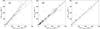 |
Fig. 1 Comparison of vsini data: a) values for the 94 stars (with spectral type equal to, or later than, B6) in common between Abt et al. (2002) and Levato & Grosso (2004). The dashed line stands for the one-to-one relation and the solid line is the result from Eq. (1); b) values for the 199 stars (with spectral type equal to, or later than, B6) in common between merged data from Abt et al. (2002) and Levato & Grosso (2004), and Royer et al. (2002b). The solid line is the result from Eq. (2); c) values for the 44 stars (with spectral type equal to, or later than, B6) in common between Huang et al. (2010) and previously merged data. The solid line is the result from Eq. (3). |
2. Rotational velocity data
The sample of stars used in the present work is primarily determined by the objects studied in Royer et al. (2002a,b, 2007, hereafter Papers I, II, and III). Because we attempt to study the rotational characteristics only of A-type stars in the MS evolutionary phase, the basis of our sample is the selection of dwarf stars with luminosity class from V to IV made in Paper III. However, the selection on the spectral class, from B9 to F2, is similar to a cut in temperature and strongly affects the distribution in the plane mass–age. The first half of the MS, corresponding to young stars, is not sampled in the hot end of the selection (spectral types B9 to A1). In order to cover the entire age sequence for stars more massive than about 2.5 M⊙ that correspond to early A and late B stars, we chose to extend the spectral type range up to B6.
The final selection of objects that comply with the purpose of the present study, however, was made using the masses and ages derived using the effective temperatures and bolometric luminosities determined in the present contribution as detailed in Sect. 3.2. We briefly recall the main characteristics of the basic sample gathered in the above cited papers in the following subsections.
2.1. v sin i data sources
Our study is based on four different sources of vsini data, from which we collected both B- and A-type stars:
-
Paper II provides a large and homogeneousvsini data set for A-type stars by merging datafrom Abt & Morrell (1995) with accuratevsini determined by Fourier transforms (FT).The first set is scaled to the later;
-
Abt et al. (2002, hereafter called ALG) provide homogeneous vsini for 1092 B-type stars derived from the FWHM of He i 4471 and Mg ii 4481 Å lines calibrated into the vsini scale of Slettebak et al. (1975). This is the extension of the work from Abt & Morrell (1995) toward B-stars and it is limited to stars brighter than V = 6.5 mag;
-
Levato & Grosso (2004, hereafter called LG) give the southern counterpart of ALG’s work: vsini for 1027 B-type stars determined with the same method;
-
Huang et al. (2010, hereafter called HGM) study rotation in a sample of B-stars (in open clusters and field). Their vsini determination was made by fitting synthetic model profiles of He i 4471 and Mg ii 4481 Å lines. Only their field star data are taken into account in this work.
This study covers the spectral types from B6 to F2. The number of stars per spectral type is given in Table 2. In the total list of our sample stars (Table 1) we provide the source of the vsini data: sources 1, 2, and 4 (and their combinations) are taken from Paper II, source 8 is taken from ALG, 16 from LG and 32 from HGM.
2.2. Merging and scaling v sin i data
Although in Paper III a merging with data from ALG was already performed to increase the number of stars corresponding to the spectral types B9 and B9.5, a new merging was performed in this work on a wider range of spectral types.
The data sets from ALG and LG were first merged, considering only stars later than B6. Then the merged sample ALG ∪ LG was merged with the A-type star sample from Paper II. Finally vsini of field B-type stars from HGM were merged with the full sample. The different vsini scales are compared in Fig. 1 for the 94 stars in common between ALG and LG, and for the 199 stars in common between Paper II and ALG ∪ LG, and for the 44 stars in common between Paper II ∪ ALG ∪ LG and HGM.
The linear regression lines between the different scales are determined with GaussFit (Jefferys et al. 1998a,b), a robust least-squares minimization program, to obtain empirical functions:  A 10% error on the vsini values was assumed for all data when using GaussFit to derive these relations.
Although the vsini from Slettebak et al. (1975) are affected by the gravitational darkening effect, Howarth (2004) showed that they are underestimated compared with more recent gravitational darkening-dependent determinations of vsini (Frémat et al. 2005). Except for the assumptions that underlie the FT method, the vsini scale defined in Paper II is independent of any other calibration. This scale is moreover confirmed by a more robust FT method (Reiners & Royer 2004) and proves to be consistent also with the vsini determinations by Erspamer & North (2003) and Fekel (2003). Recent results from Díaz et al. (2011) provide accurate measurements of vsini using FT of the cross-correlation function for 251 A-type stars in the southern hemisphere. Their method is much less sensitive to blends than the individual line measurements made in Paper I, and their vsini values are 5% higher for vsini > 150 km s-1. This effect is smaller than the 10% error assumed for our merged sample, however, and because of the late knowledge of their results, we chose to leave our scale unchanged. We therefore used the FT scale of vsini defined in Paper II and used Eqs. (1)–(3) to scale all vsini data to this scale. The full sample contains 2014 stars and the homogenized vsini are given in Table 1.
2.3. Chemically peculiar and binary stars
In order to have a stellar sample that is as clean as possible from objects whose rotation could have been modified by tidal or magnetic braking, all known chemically peculiar stars (CP) and “close” binary stars (CB) were discarded. The selection was made with the same criteria as we used in previous papers.
CP stars (chemically peculiar stars): the catalog of Ap and Am stars from Renson & Manfroid (2009) and the spectral classifications given by ALG, LG and HGM were used to identify peculiar stars.
CB stars (“close” binary stars): This category of stars was selected on criteria based on HIPPARCOS and spectroscopic data. Most of the selected stars are in the HIPPARCOS catalog (ESA 1997). The binaries detected by the satellite with ΔHp < 4 mag are flagged as CB stars. The Ninth Catalog of Spectroscopic Binary Orbits (Pourbaix et al. 2004) was used to complete the identification.
All stars that do not obey CB or CP criteria are simply called “normal”. The question of identification completeness is studied in Paper II, which concludes that the fraction of CP stars to all stars in the merged sample is fairly constant for all magnitudes brighter than V = 6.5 mag and represents roughly 15% of the objects.
3. Fundamental parameters
List of the 2014 B6- to F2-type stars, with their spectral type and fundamental parameters (extract).
In the present contribution, the rotational properties of stars are studied as a function of age and mass following a statistical approach. The studied objects were gathered into groups that contain enough data to warrant that the projection effect in vsini can be statistically corrected. The subtle deviations caused by fast rotation effects, in particular those affecting the vsini parameter (Zorec et al. 2002; Frémat et al. 2005), can easily be obliterated in the averaging process by the uncertainties affecting the individual fundamental parameters. Therefore we inferred stellar masses and ages from the apparent effective temperatures and bolometric luminosities in the present approach as if the objects were at rest.
3.1. Effective temperatures and bolometric luminosities
 |
Fig. 2 Color-effective temperature diagram for the single normal stars selected for the present study. |
 |
Fig. 3 Comparison of effective temperatures calculated in this paper from the uvby − β photometry and those for 135 stars obtained using bolometric fluxes. The dashed line is the one-to-one relation. |
The effective temperatures of stars were derived using uvby–β Strömgren photometry and the calibration of Strömgren photometric color indices into Teff. The calibrations employed are from Moon & Dworetsky (1985), its revisited version for some spectral types and luminosity classes obtained by Castelli (1991), and the corrected and extended one for the hottest stars by Napiwotzki et al. (1993). The adopted Teff for a given star is the average obtained as follows. The (b − y), m1, c1 and β indices were taken from Hauck & Mermilliod (1998) and used with their respective uncertainty. The photometric indices were used following a Monte Carlo sampling within intervals (⟨X⟩ − 2σX, ⟨ X ⟩ + 2σX), where σX is the dispersion of each individual photometric index X. For each star we obtained 6500 Teff-determinations, whose average and the corresponding dispersion are the adopted Teff ± σTeff values presented in Table 1. In Fig. 2 we show the obtained effective temperatures against the photometric colors (b − y) corrected for interstellar extinction. For some stars in the sample of Huang et al. (2010)uvby–β photometry is not available, so that we used the Teff estimates derived by these authors.
Sometimes, more or less systematic deviations can be expected between the effective temperatures determined from photometric indices with those based on bolometric fluxes (Zorec et al. 2009). While the details of the stellar energy distribution can be important when Teff is determined with photometric indices, they have a marginal incidence in the Teff-determination with bolometric fluxes (Frémat & Zorec 2003; Frémat et al. 2003). We compared the effective temperatures of 135 stars obtained in this work with those determined with bolometric fluxes. Techniques for determining effective temperatures with integrated bolometric fluxes are given in Zorec et al. (2009) and they are presently used to determine the effective temperature of 600 A- and F-type stars (in prep.). The comparison (Fig. 3) shows a great consistency.
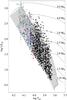 |
Fig. 4 HR diagram of the studied stars. Only the single normal stars in the shaded region were selected for the present study. Filled circles are for stars in the sample studied by Royer et al. (2007). Open circles, open diamonds and asterisks stand for complementary stars taken from Abt et al. (2002), Levato & Grosso (2004) and Huang et al. (2010) respectively. The evolutionary tracks are from Schaller et al. (1992). |
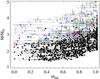 |
Fig. 5 Distribution in the (t/tMS,M/M⊙) plane of the data concerning the single normal stars selected for the present study. The error bars in both coordinates are indicated in gray. The symbols have the same meaning as in Fig. 4. |
The bolometric luminosity of stars is estimated with 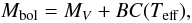 (4)where MV is the visual absolute magnitude and BC(Teff) is the bolometric correction (Lang 1992). To calculate MV we used (i) the apparent visual magnitude of the UBV photometry and the corresponding uncertainty; (ii) the HIPPARCOS parallaxes recently re-determined by van Leeuwen (2007) and taking into account the respective uncertainties; (iii) the interstellar color excess E(B − V) estimated using the uvby–β photometry and the calibration of intrinsic colors by Moon & Dworetsky (1985). Each adopted Mbol magnitude is the average of all determinations by Eq. (4) following a Monte Carlo sampling of the uncertainties affecting Teff and the parameters entering Pogson’s relation for MV. The adopted bolometric luminosity parameter log L/L⊙, given in Table 1 with its 1σ uncertainty, was derived by adopting
  mag.
mag.
3.2. Stellar masses and ages
To infer the individual stellar masses and ages, we used the pairs (Teff,log L/L⊙) obtained above with their respective 2σ deviations as entries in the evolutionary diagrams of non-rotating stars calculated by Schaller et al. (1992) that we display in Fig. 4. The interpolation of masses and ages also proceeds with a Monte Carlo sampling of the (Teff,log L/L⊙) entries. Table 1 gives the average (M/M⊙,t/tMS), i.e. mass and fractional age parameters with the 1σ dispersion that are the results from each interpolation procedure. We use here the notation t for the age in years, and t/tMS is the life span from the ZAMS to the TAMS (terminal age main sequence) of a star with the given mass M/M⊙. Figure 5 shows the distribution in the mass–age diagram of the MS stars used in the present study. The vertical cuts in effective temperature in Fig. 4 that appear because of the selection based on MK spectral type are reflected in Fig. 5 by the limits in mass varying with age. Table 2 gives some statistical estimators that describe the characteristics of the stellar mass distribution tabulated against the spectral types of the present analysis.
The stars with large error bars on mass and/or age (σ/M⊙ ≥ 0.3, σt/tMS ≥ 0.15) were discarded for the next steps of this work.
Parameters of the mass distributions in different spectral type intervals.
3.2.1. Uncertainties regarding the stellar masses and ages
Mass and age estimates using evolutionary tracks with rotation for a test star with apparent rotation-less mass M = 3 M⊙.
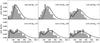 |
Fig. 6 Distributions of rotational velocities for normal stars in different mass subsamples: shaded histograms are the observed vsini; solid thick lines are the distributions of equatorial velocities and the gray strips are their associated variability bands. The dashed lines stand for the Maxwellian fit, whose parameters are given in Table 4. The mass range for each subsample is indicated in the corresponding panel, together with the number of stars. The histograms are normalized to fit the probability density scale. |
Because models of stellar evolution with rotation can produce evolutionary tracks that can differ significantly from those without rotation (Maeder & Meynet 2000; Ekström et al. 2008, 2011), we may wonder whether the masses and ages obtained for our sample stars, which can be intrinsic rapid rotators, are still realistic. Because we do not know the actual internal rotation of a given star in advance, whatever uncertainty we can estimate will necessarily be model-dependent. We can then recall that the most frequently used models (cf. Maeder & Meynet 2000; Ekström et al. 2008, 2011) are based on two strong assumptions: (i) all stars initiate their evolution in the MS as rigid rotators, which means the total rotational energy stored in the object is strongly limited (see discussion in Sect. 5.4); (ii) the redistribution of angular momentum proceeds only over barotropic surfaces and produces only “shellular” internal rotation laws. We have calculated the masses and rotation-dependent masses and fractional ages t(Ω)/tMS(Ω) suggested by these models for a test star that according to rotation-less models has a mass M = 3 M⊙ and lies at evolutionary phases t/tMS = 0.2, 0.5 and 0.8. The obtained results are given in Table 3. From this table we can conclude that the parameters based on rotation-less models used in the present work (M/M⊙,t(Ω)/t/tMS) may slightly underestimate stellar masses in the first half of the MS, and that the differences are larger for a higher ratio Ω/Ωcrit. Masses can be slightly overestimated for stars in the second half of the MS. Because the actual ratio Ω/Ωcrit is not known, the stellar mass and its uncertainty are on average ⟨ M ⟩ = 3.01 ± 0.12 M⊙. In Table 3 we note that rotation-dependent ratios can be systematically lower than those derived from rotation-less models and the differences are larger the closer the stars are to the TAMS and the higher the ratio Ω/Ωcrit. The effect of neglecting rotation on the derivation of M/M⊙ and t/tMS for other stellar masses can be seen in Fig. 6 of Zorec et al. (2005), where the authors studied Be stars, which are considered as paradigms for rapidly rotating MS stars. We note, however, that the fraction of program stars in the present work with Ω/Ωcrit ≈ 1.0 must probably be very low, because the fraction of Be stars among the B-type star population is low (Zorec & Briot 1997). On the other hand, as soon as Ω/Ωcrit ≲ 0.9, age differences become δ(t(Ω)/tMS) ≲ 0.1, which are on the same order or smaller than the age-bins used to estimate the averages ⟨ v ⟩ of true equatorial velocities in the following sections.
Parameters of the 1D velocity distributions for normal stars as a function of the stellar mass.
3.2.2. Determining fundamental parameters with rotation-dependent evolutionary tracks
The use of evolutionary tracks with rotation implies that we have an estimate of the true equatorial velocity v of the studied star. These tracks are given in terms of bolometric luminosities and effective temperatures averaged over the rotationally deformed object as a function of age and rotational velocities in the ZAMS. Accordingly, the observed apparent aspect angle-dependent effective temperature and bolometric luminosity must be corrected for rotational effects to derive their counterparts for the corresponding rotation-less object (Frémat et al. 2005; Zorec et al. 2005). In turn, these must be averaged over a rotationally deformed star, whose degree of geometrical deformation is measured by the ratio v/vcrit(M,t), where vcrit(M,t) is the stellar critical equatorial velocity. Using the curves representing the evolution of the ratio v(M,t)/vcrit(M,t), the stellar velocity ratio in the ZAMS must be identified. Only evolutionary tracks for this specific initial velocity ratio, and for several masses around the sought one, can finally be used to interpolate the mass and age of the studied object. This operation implies a long iteration procedure, where the stellar mass M/M⊙, its age t/tMS and the inclination angle i of the rotational axis are iterated simultaneously. Knowing that on the one hand only a small fraction of program stars may be very rapid rotators, and on the other hand this iteration will not bring significant improvements in the estimate of masses and ages of the remaining stars, the approach used in the present work seems justified.
3.3. The v sin i parameters and the rapid rotation
The estimates of vsini parameters can also be affected by the rapid rotation. Rapid rotation induces temperature and gravity inhomogeneities in the stellar surface known as the “gravity darkening effect”. Owing to the lowering induced on the local effective temperatures in the equator, these regions do not contribute efficiently to the Doppler rotational broadening of spectral lines. The apparent vsini of rapid rotators must then be corrected for this underestimation (Frémat et al. 2005). This correction can increase our estimates of v/vcrit only if it can be demonstrated that in each bin used to average the apparent vsini parameters, the number of rapid rotators with actual ratios Ω/Ωc ≳ 0.8 represents a significant fraction of objects.
4. Distributions of rotational velocities
In Paper III, distributions of rotational velocities were obtained by dividing the stellar sample into groups of spectral types and mixing stars of all ages in the MS life span. However, the spectral type of a star changes during the MS life span, so that in a given group objects with different masses and ages can display roughly the same apparent spectral type. To have a better representation of the percentage of stars as a function of the rotational velocity per mass-groups and study the distribution of rotational velocities as a function of the stellar mass, the sample of normal stars defined above was divided into overlaping mass intervals that run from 1.6 to 3.85 M⊙. The limits of the intervals together with the corresponding number of stars are given in Table 4. For each subset, the distribution of vsini was processed in a way similar as in Paper III:
-
the histogram was smoothed using a Gaussian kernel estimatorand smoothing parameter ĥ defined by Bowman & Azzalini (1997)1, and variability bands were estimated (Bowman & Azzalini 1997);
-
the smoothed distribution was rectified from the projection effect, assuming randomly oriented rotation axes, with the Lucy-Richardson method (Lucy 1974; Richardson 1972);
-
the rectified distributions were fitted by a sum of two Maxwellians to derive the position of the mode(s) and the proportion of fast and slow rotators if a significant bimodality is present. The Maxwellian distribution used to fit the fast part of the velocity distribution has an additional lag parameter ℓ, to be able to shift it toward higher velocities2.
The distributions are shown for some of the mass intervals in Fig. 6, and the results of the fits are given in Table 4. An overview of the distribution of the rotational velocities as a function of mass for the stellar sample in the present work is displayed in Fig. 7. In this figure the full MS life span is considered: 0 ≤ t/tMS ≤ 1. The color scale represents the density in the one-dimensional normalized distributions: the bluer the region, the smaller the number of stars and vice versa toward the red scale.
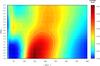 |
Fig. 7 Distribution of true rotational velocities v for normal stars as a function of the stellar mass M/M⊙. The color scale represents the density in the one-dimensional normalized distributions. The bluer the region, the smaller the number of stars and vice versa for the red colored scale. White solid lines follow iso-density contours. |
Parameters of the 1D velocity distributions for all stars (normal, CP and CB) as a function of the stellar mass.
We clearly notice in Fig. 7 two main groups of stars as a function of stellar mass with a transition occurring at M ≈ 2.5 M⊙. In the low-mass part of the diagram, the distribution is unimodal and there is a striking lack of objects in the 0 ≲ v ≲ 100 km s-1 interval of velocities. This gap in the distribution in the plane (v,M) is also noticeable, although less pronounced, in (vsini, spectral type) as shown in Royer (2009). With the aim of testing the effect of our selection of normal stars on the resulting distributions, the same process was applied to all stars (normal, CP and CB). Table 5 gives the results of the fits for the same mass intervals. The lack is still present even when CP and CB stars are not removed from the sample, although some minor overdensities occur for v ≲ 40 km s-1. The effect of discarding CP and CB stars cannot account for the lack of slow rotators, and we conclude that stars with low rotational velocities were not created in the space volume scrutinized with our data.
For stars with M ≳ 2.5 M⊙, the bimodality of the velocity distribution distinctly appears. The proportion of the slow rotators increases to 20% around M ≈ 2.8 M⊙ and decreases toward higher masses. The selection of normal stars removes a large proportion of slow rotators (0 ≲ v ≲ 100 km s-1) in this mass range, as seen when comparing the percentage of the slow rotator Maxwellian distributions from Tables 4 and 5, but the bimodality remains significant.
The fast rotator mode of the equatorial velocity distribution for normal stars, μr, behaves monotonically over the full range of mass and smoothly increases with stellar mass. This variation can be fitted by a linear relation in the mass range 1.6–3.5 M⊙:  (5)
(5)
4.1. Normal versus peculiar stellar populations
It was argued by Abt (2009) that slowly rotating A0–A3 “normal” stars are stars that did not have enough time to become Ap or Am stars yet, and that Ap(SrCrEu) stars need about half of their MS lifetime to show their chemical peculiarity. This effect would bias the distributions of rotational velocities when one considers only “normal” stars and applies a selection by age.
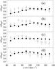 |
Fig. 8 Mean age ⟨ t/tMS ⟩ per bin of vsini for different mass intervals (taken from Table 4): a) 2 < M/M⊙ < 2.4; b) 2.2 < M/M⊙ < 2.6; c) 2.35 < M/M⊙ < 2.85; d) 2.55 < M/M⊙ < 3.05. Filled circles stand for normal stars, whereas open squares represent CP stars. The bins in vsini are 40 km s-1 wide. Solid lines are the results of linear fits on normal stars with vsini ≤ 110 km s-1 and dashed lines the results of the fits for CP stars with vsini ≥ 90 km s-1. |
The averaged age on the MS as a function of vsini was derived for different mass intervals in our sample, considering normal stars and CP stars separately (Fig. 8). In the first two mass intervals (2 < M/M⊙ < 2.6) there is a significant and systematic shift between normal and CP stars for vsini ≲ 100 km s-1, CP being on average older by 10% of tMS. One should bear in mind that when deriving the fundamental parameters of our targets, normal and CP stars are treated in the same way. Therefore, the bolometric luminosity of CP stars can be overestimated. Landstreet et al. (2007) indeed show that the bolometric correction for Ap stars is smaller than the one calibrated by Lanz & Catala (1992) by an amount of about 0.2 mag. Their age derived from their position in the HR diagram may consequently be also overestimated.
On the other hand, a trend is seen in the variation of the mean age of normal stars in the first mass interval (2 < M/M⊙ < 2.4). It increases monotonically from 53% to 68% of tMS between vsini = 50 and 110 km s-1, and remains constant for faster rotators. This trend is less pronounced in the next mass bin, and completely disappears for more massive stars. This trend agrees with that postulated by Abt (2009). Moreover, the variation of the mean age with rotation is recovered using vsini, therefore the projection effect can lessen the slope. But the selection here was made using mass and age. According to the evolutionary tracks in Fig. 4, the A0–A3 spectral types will correspond to different stellar masses if stars are close to the ZAMS or near the TAMS.
This trend does not seem to explain the bimodality observed in Figs. 6 and 7. According to Table 4, the bimodality reaches its maximum (in terms of percentage of the full distribution) in the mass bin 2.55 < M/M⊙ < 3.05, for which no obvious trend is seen in Fig. 8d.
4.2. Evolution of the distributions of rotational velocities
In the distributions shown in Fig. 6 stars are not distinguished by their ages. Below, stellar ages are taken into account in two different ways: (i) by studying the changes of the rotation velocity distributions as a function of time (this section); (ii) by studying the evolution from the ZAMS to the TAMS of the average rotational velocities per mass (Sect. 5).
The evolution of the distributions of rotational velocity during the MS life time is studied separately for the two groups of stars identified in Fig. 7. The cut in mass was chosen to be M ≳ 2.4 M⊙, however, to gather enough stars in the high-mass part. We obtained distributions of v for each mass group by separating the stars into three age intervals (Fig. 9). They were chosen so that the number of stars in each of them enabled us to rectify the distributions from the projection angle effect. As seen in Fig. 5, the young part of the diagram is poorly sampled. Hence the first bin is large, 0 < t/tMS < 0.5, to warrant statistical reliability. The two mass bins behave quite differently as a function of age. Table 6 gives the parameters that characterize the subsamples and their velocity distributions.
The low-mass star v distribution does not vary significantly in shape with age, and remains unimodal from ZAMS to TAMS. It shows an acceleration, however. The mode of the distribution increases from about 150 km s-1 for 0 < t/tMS < 0.5, to 170 km s-1 for 0.5 < t/tMS < 0.8 and to about 185 km s-1 for 0.8 < t/tMS < 1.
The high mass v distribution does exhibit significant changes as a function of age. The bimodality is very clear among stars younger than t/tMS < 0.8, whereas the two peaks blend near the TAMS (0.8 < t/tMS < 1). Slowly rotating stars are present at any age, but the fast rotating part of the distribution decelerates with increasing age. In terms of positions of the mode, the distribution peaks at about 240 km s-1 for the younger half (t/tMS < 0.5), and stagnates at about 190 km s-1 for the older part. In terms of median of the full distribution, however, the deceleration is continuous and the median v decreases from 250 km s-1 for 0 < t/tMS < 0.5, to 210 km s-1 for 0.5 < t/tMS < 0.8 and to 185 km s-1 for 0.8 < t/tMS < 1.
Using these distributions, the ratio of the average velocity of the fast rotating component (derived from the formula of the Maxwellian distribution) over the average velocity of the full component was derived. This ratio is characterized by the factor κr, which allowed us to correct in Sect. 5.2 the mean values of rotational velocities in mixed samples encompassing slowly and rapidly rotating stars. It corrects the curves of rotational velocities against stellar ages for the effect carried by the slowly rotating stars, so as to derive distributions and related modes for the rapidly rotating stars only.
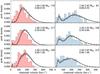 |
Fig. 9 Distributions of rotational velocities as a function of age for two mass subsamples. Left panels correspond to the low-mass bin: 1.6–2.4 M⊙ and right panels correspond to the high-mass bin: 2.4–3.85 M⊙. As in Fig. 6, shaded histograms are the observed vsini; solid thick lines are the distributions of equatorial velocities v and the gray strips are their associated variability bands. The mass range for each subsample is indicated in the corresponding panel together with the number of stars, and below, the age interval is indicated and goes from young stars (0 < t/tMS < 0.5) in upper panels to stars close to the TAMS (0.8 < t/tMS < 1) in lower panels. The histograms are normalized to fit the probability density scale. |
5. Evolution of the rotational velocities compared with models
In a first attempt, we tried to apprehend possible dependencies of the evolution with age of rotational velocities for different masses through the v/vcrit velocity ratio, where vcrit is the time- and mass-dependent critical equatorial rotational velocity. In a second approach, we studied the v/vZAMS velocity ratio, where vZAMS is the equatorial rotational velocity on the ZAMS.
The velocity ratios v/vcrit and v/vZAMS were compared with model predictions for three different regimes of internal redistribution of the angular momentum. The first two predictions are for extreme redistributions and are detailed in the present discussion. The third type of models were calculated by Ekström et al. (2008) for stars with 3 M⊙, the only common mass with the present paper.
The ZAMS was considered as the initial state of the MS stellar evolutionary phase. Nevertheless, as a consequence of all possible physical conditions prevailing during the evolutionary stages preceding the ZAMS, a given star on the ZAMS could be either a rigid rotator or a differential rotator. If the star is a differential rotator, the total angular momentum stored in the object can be higher or lower than the limiting value supported by a critical rigid rotator. The characteristics of the stellar structure depend on the amount of rotational energy stored and on the internal distribution of the angular velocity. The competition between gravitational and centrifugal forces determines the final stellar internal structure, the meridional circulation, and the mixing phenomena of chemical elements that put constraints to the subsequent stellar evolution in the MS (cf. Maeder & Meynet 2000).
The mass-loss rates inferred for A-type stars are on the order of 10-12 to 10-10 M⊙ yr-1 (Lanz & Catala 1992; Lamers & Cassinelli 1999), which for evolutionary time scales ranging from 108 to some 109 yr implies that the amount of angular momentum removed in these objects during their MS life span is probably negligible on average. We assumed then that all studied stars evolve during the MS phase conserving their total angular momentum.
The amount of rotational kinetic energy stored by a star is currently estimated using the ratio τ = K/|W|, where K is the kinetic energy and W is the gravitational potential energy. At rotational energies approaching τ ≈ 0.27, the object is dynamically unstable. For τ ≈ 0.14 it becomes secularly unstable, in the sense that its axial symmetry can be broken and transformed into a three-axially symmetric body (Tassoul 1978). If at any time during the MS evolution a star has a total angular momentum higher than permitted by the critical rigid rotation, the star is said to evolve as a neat differential rotator. We refer to the evolution at low rotational energy regime if stars have  , otherwise they will be said to evolve at high rotational energy. The notation
  stands for the critical, or upper possible energy born by a rigid rotator, which ranges from
  to 0.0053 for stars with masses from M = 1.5 to 3 M⊙, respectively. Assuming that stars are permanently axisymmetric, the evolution at high-energy regime implies that
  .
.
In the present discussion we assumed that stars evolve in the MS at low rotational energy regime, i.e. they have . Moreover, in our calculations we still limited the total angular momentum to  , where for a given mass,
  corresponds to the angular momentum supported by a critical rigid rotator on the TAMS. This choice is mandatory for stars that are assumed to be rigid rotators on the ZAMS and they evolve in the MS by conserving the total angular momentum. In fact, a star steadily becomes more centrally condensed and its radius is enlarged as it evolves from the ZAMS to the TAMS. This decreases the upper limit of total angular momentum with time that the star can bear.
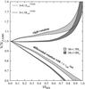 |
Fig. 10 v/vZAMS ratio of equatorial rotational velocities as a function of the t/tMS time ratio in the MS for stars with masses from M = 1.5 to 3 M⊙. vZAMS is the equatorial rotational velocity on the ZAMS, t is the stellar age and tMS is the time that a star of given mass M can remain in the MS. Two extreme cases are represented: stars evolving as rigid rotators (instantaneous complete angular momentum redistribution) and as differential rotators without any angular momentum redistribution. Dashed lines represent the limits for J/M → 0, while the solid lines are for stars that on the ZAMS have a specific angular momentum that in the TAMS becomes the critical one. |
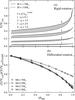 |
Fig. 11 Theoretical evolution of the v/vcrit velocity ratio calculated for several stellar masses. a) Dependence with time of the v/vcrit ratio for several values of the total specific angular momentum J, when stars evolve as rigid rotators all long the MS phase; b) evolution of the ratio v/vcrit normalized to its value on the ZAMS when rotators conserve the angular momentum by shells. |
5.1. Two limiting cases for the evolution of the equatorial rotational velocities
Two simple and extreme cases of the evolution of the surface angular velocity can be considered, depending on the way the star redistributes its angular momentum during the MS evolutionary phase. For the limited values of rotational energy stored by the stars on the ZAMS stated above, , this can happen in two ways: (i) by entirely redistributing its angular momentum at any instant; (ii) by impeding any exchange of angular momentum among the stellar shells, so that each of them conserves its specific angular momentum. In the first case the star evolves as a rigid rotator, while in the second case, we say the star evolves as a simple differential rotator.
5.1.1. Stars evolving as rigid rotators
The equatorial velocity at a time t elapsed from the ZAMS (t = 0) in a star rotating as a rigid rotator is roughly given by ![Mathematical equation: \begin{equation} \frac{\veq(t)}{\vzams} =\left[\frac{R(t)}{R_{\rm ZAMS}}\right]\left[\frac{I_{\rm ZAMS}}{I(t)}\right], \label{veq_rig} \end{equation}](/articles/aa/full_html/2012/01/aa17691-11/aa17691-11-eq145.png) (6)where [v(t),vZAMS] , [R(t),RZAMS] and [I(t),IZAMS] are the stellar equatorial linear rotational velocity, the radius and the moment of inertia at time t and at the ZAMS, respectively. We calculated two-dimensional models of stars with rigid rotation as detailed in Appendix A. Figure 10 shows the evolution of the ratio v/vZAMS for stars with masses M = 1.5 and 3 M⊙ that conserve their total angular momentum during the MS evolutionary phase. The calculation was made for values of the angular momentum parametrized as
(6)where [v(t),vZAMS] , [R(t),RZAMS] and [I(t),IZAMS] are the stellar equatorial linear rotational velocity, the radius and the moment of inertia at time t and at the ZAMS, respectively. We calculated two-dimensional models of stars with rigid rotation as detailed in Appendix A. Figure 10 shows the evolution of the ratio v/vZAMS for stars with masses M = 1.5 and 3 M⊙ that conserve their total angular momentum during the MS evolutionary phase. The calculation was made for values of the angular momentum parametrized as  , where q takes the values 0.1 and 1. For objects undergoing total redistribution of the angular momentum, the velocity ratio v/vZAMS increases very slowly or remains nearly constant over the first two-thirds of the MS evolutionary period. Only in the last third of the MS phase do the changes of the stellar structure as a function of the angular momentum produce some effects on the equatorial velocity, which slightly depend on the stellar mass.
The variation of the v/vcrit ratio in rigid rotators of different masses and with total angular momenta (q = 0.1, 1/3, 2/3, 1) is plotted in Fig. 11a. The v/vcrit velocity ratio of rigid rotators remains nearly unchanged during the first two-thirds of the MS evolutionary phase, and increases sensitively only in the last third of the MS. However, (v/vcrit)ZAMS clearly depends on the total angular momentum J.
5.1.2. Stars evolving as simple differential rotators
The geometrical deformation of the stellar surface mainly depends on the specific angular momentum on the surface (Zorec et al. 2011a,b). Owing to the particular differential rotation assumed here, the specific angular momentum will become increasingly centrally condensed, so that the amount left in the surface will decrease strongly as the star evolves from ZAMS to TAMS. A simple account of the stellar deformation induced by the differential rotation could in principle be performed using a homoeoidal description of the internal density distribution (Chandrasekhar 1969), where the specific angular momentum is constant over spheroidal shells. However, owing to the fairly small effects carried by the rotation studied here on the stellar shape, we assumed that stars are spherical. The angular momentum of a spherical shell of width dr is  (7)where ρ(r) and Ω(r) are the density and the angular velocity at radius r. Ω(r) is assumed to be uniform over each shell, i.e. “shellular” distribution of the angular velocity. If r and r′ are the radii at times t and t′ of the same shell, whose mass dM(r) = 4πρ(r)r2dr and angular momentum are conserved, we have
  (8)which for the equatorial velocity at t and t′ in the stellar surface implies that
 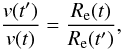 (9)where Re(t) and Re(t′) are the equatorial radii of the star at times t and t′, respectively. The change of the internal angular velocity as described by Eq. (8) induces a small variation on the moment of inertia that is taken into account as described in Appendix B. The variation of the equatorial velocity with time thus obtained and normalized to its value on the ZAMS is plotted in Fig. 10. The time dependent v/vZAMS curves are also function of the stellar mass, while they are quite independent of the value of J.
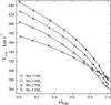 |
Fig. 12 Critical equatorial rotational velocities of stars with different masses as a function of age in the MS. At each t/tMS the objects are assumed to be rigid rotators. |
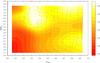 |
Fig. 13 Distribution of the ratio v/vcrit of true rotational velocities as a function of the fractional age in the MS evolutionary phase for normal stars in the mass interval 1.7 ≤ M ≤ 3.3 M⊙. The filled circles are the average positions of the stars in running boxes with bins of 0.15 in t/tMS and 0.5 in M/M⊙. |
In Fig. 11 we show the variation of v/vcrit as a function of time for stars with masses from M = 1.5 to 3 M⊙, and several values of the angular momentum with q ranging from 0.1 to 1. Although the ratio v/vcrit depends on the value of J, its variation with time has a tiny dependence with mass. To demonstrate this small dependence with mass, the curves in Fig. 11b are normalized to the respective values on the ZAMS: [v(M)/v(M)crit] ZAMS. Owing to the low values of J chosen here, model stars can never have a critical specific angular momentum in the equator. For internal rotation laws given by Eq. (8) this can happen only for much higher values of J, which means that in this case the stars behave in the MS always as neat differential rotators.
5.2. Observed evolution of rotational velocities vs. predicted extreme angular momentum redistribution regimes
A general picture derived using observations of the evolution of rotational velocities in the MS as a function of mass is given in Fig. 13, where the average ratio of true rotational velocities ⟨ v/vcrit ⟩ is shown as a function of the fractional age t/tMS in the MS for masses in the interval 1.7 ≤ M ≤ 3.3 M⊙. vcrit is the equatorial critical velocity given by ![Mathematical equation: \begin{equation} \vc = 436.7\left(\frac{M}{\Msol}\right)^{1/2}\left[\frac{R_{\odot}}{R_{\rm crit}(M,t)}\right]^{1/2} \quad \kms, \label{crit_vel_fo} \end{equation}](/articles/aa/full_html/2012/01/aa17691-11/aa17691-11-eq169.png) (10)where Rcrit(M,t) is the stellar radius at critical rotation. For each star, the mass- and time-dependent critical radius Rcrit(M,t) was determined using two-dimensional models of rigidly rotating stars, whose characteristics are given in Appendix A. Figure 12 plots vcrit(M,t) against t/tMS for several stellar masses ranging from M = 1.5 to 3 M⊙.
(10)where Rcrit(M,t) is the stellar radius at critical rotation. For each star, the mass- and time-dependent critical radius Rcrit(M,t) was determined using two-dimensional models of rigidly rotating stars, whose characteristics are given in Appendix A. Figure 12 plots vcrit(M,t) against t/tMS for several stellar masses ranging from M = 1.5 to 3 M⊙.
To obtain the diagram of average true rotational velocities ⟨ v/vcrit ⟩ shown in Fig. 13, each observed vsini parameter was divided by the corresponding vcrit(M,t). The values were averaged in running boxes with age bins of 0.18 for t/tMS < 0.3 and 0.15 for t/tMS > 0.3 and mass bins of 0.5 M⊙. These intervals are wide enough to ensure that the number of stars entering each average leads to statistically reliable transformations from ⟨ vsini ⟩ to ⟨ v ⟩ and they are narrow enough to warrant that useful information on the evolutionary characteristics of rotation is hardly not obliterated. The true equatorial velocities come from the average of the vsini parameter corrected for sini according to the statistical principles given by Chandrasekhar & Münch (1950). The two-dimensional distribution was smoothed with a smoothing parameter derived as in Sect. 4 (see Bowman & Azzalini 1997).
The two mass regions already identified in Fig. 7 depict in Fig. 13 an evolution of ⟨ v/vcrit ⟩ with different characteristics. The limit between these regions is roughly at M ≈ 2.5 M⊙. To obtain a better insight on the characteristics of the evolution of the ⟨ v/vcrit ⟩ ratio in each of these mass-intervals, constant mass curves were extracted from Fig. 13 for three stellar masses: 2, 2.5 and 3 M⊙, which represent the average evolution of the ratio ⟨ v/vcrit ⟩ as a function of time t/tMS and also describe the most typical aspects observed of the evolution of ⟨ v/vcrit ⟩ . These curves can be taken as tracers of the evolution of the average true rotational velocity against the fractional age t/tMS. However, for masses M ≥ 2.5 M⊙, these curves carry information on the evolution of two mixed groups of stars that we have already differentiated into slowly and rapidly rotating populations, of which the last is the most numerous one. Because the evolution of the rotational velocity in these stellar groups can present systematic differences, we aimed at obtaining the ⟨ v/vcrit ⟩ curves that represent only the rapidly rotating stellar population. To this end, we used the correction factor κr (Table 6) that converts the mean values ⟨ vs + r ⟩ of mixed slowly and rapidly rotating stars “s+r” to the searched rapid one ⟨ vr ⟩ = κr(t) × ⟨ vs + r ⟩ . The values calculated for the mid-time of each age interval were then interpolated for the required ages in the time interval 0 ≤ t/tMS ≤ 1. Because κr(t) remains fairly constant over the first two thirds of the MS lifetime span, and the curves of average rotational velocities that we study here were normalized to the average velocity on the ZAMS, only the ⟨ v ⟩ velocities in the last evolutionary phases on the MS do undergo some little changes as compared to the original mixed average velocity distributions.
The corrected ⟨ v/vcrit ⟩ curves as a function of the fractional age t/tMS are presented in Fig. 14, where the vertical error bars give an insight on the uncertainties affecting the ⟨ v/vcrit ⟩ -ratio determination and the horizontal error bars are the averaged σt/tMS (from Table 1) in each bin. In this figure are superimposed the bands that correspond to the evolution of v/vcrit ratio for rigid rotators of masses from M = 1.5 to 3 M⊙ previously shown in Fig. 11. They represent two angular momenta:  (middle of the diagram) and
  (lower right corner). Even if in Fig. 14 the evolution of simple differential rotators is not shown, we notice that the evolution of ⟨ v/vcrit ⟩ differs strongly from what is predicted from the two extreme possibilities of angular momentum redistribution described in Sect. 5.1. In fact, in the first third of the MS and for both mass-groups, the ratio ⟨ v/vcrit ⟩ increases faster than suggested by the theoretical predictions. The ⟨ v/vcrit ⟩ ratio of stars with M = 2 M⊙ increases monotonically until the TAMS, while in stars with M ≥ 2.5 M⊙ it reaches a maximum at t/tMS ≈ 0.3. There is then a decrease that lasts roughly Δt/tMS ≈ 0.2, followed by a uniform value of ⟨ v/vcrit ⟩ until the TAMS.
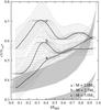 |
Fig. 14 Evolution of the equatorial velocity ratio ⟨ v/vcrit ⟩ in the MS life time span. The ratios of true equatorial velocities are calculated for three masses: 2 M⊙, 2.5 M⊙ and 3 M⊙. The shaded regions correspond to the theoretical evolution of the v/vcrit ratio in rigid rotators plotted in Fig. 11, whose total angular momenta are |
We calculated the mass- and time-dependent vcrit corresponding to all points in the curves of Fig. 14 and derive the evolution of the average true equatorial velocities ⟨ v ⟩ normalized to ⟨ v ⟩ ZAMS for the same masses. The result is plotted in Fig. 15, where we also show the respective uncertainties. In this figure are superimposed the sequences of model v/vZAMS variations for rigid (middle of the figure), and for simple differential rotators (lower left corner) previously shown in Fig. 10.
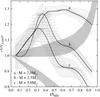 |
Fig. 15 Evolution of the equatorial velocity ratio ⟨ v/vZAMS ⟩ in the MS life time span, where vZAMS is the true equatorial velocity of stars on the ZAMS. The average true equatorial velocities were calculated for the same masses as in Fig. 14. The shaded regions correspond to the theoretical evolution of the v/vZAMS ratios shown in Fig. 10: rigid rotators (middle), simple differential rotators (lower left corner). |
The common characteristic of ⟨ v/vZAMS ⟩ curves seen in Fig. 15 is that for all masses they increase fast in the first third of the MS phase. For stars with M ≥ 2.5 M⊙ (curves b and c), the ratio ⟨ v/vZAMS ⟩ decreases more or less monotonically in the second half of the MS phase. Owing to the shown uncertainties, we cannot be sure that the slopes reveal a slightly faster decrease than predicted for simple differential rotators. If it were actually the case, this decrease could imply some redistribution of angular momentum toward the center of stars, provided that in the meantime no strong loss of angular momentum through stellar winds occurs. For stars with M = 2 M⊙ (curve a), ⟨ v/vZAMS ⟩ remains almost constant from t/tMS ≈ 0.4 until t/tMS ≈ 0.7, and decreases slowly as the evolution approaches the end of the MS phase. This decrease follows the slope of simple differential rotators very closely, nearly as if the stars were not undergoing any redistribution of the angular momentum in the external layers during the final stages of their MS phase.
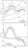 |
Fig. 16 Comparison of the observed evolution of equatorial velocity ratios in the MS life time span for stars with M = 3 M⊙ inferred from observations with theoretical ones calculated by Ekström et al. (2008) for different v/vcrit on the ZAMS. a) Evolution of ⟨ v/vcrit ⟩ ratios; b) evolution of ⟨ v/vZAMS ⟩ ratios. |
In Figs. 14–16 we show the uncertainties associated to the averages of fractional ages t/tMS, which in all cases are σt/tMS ≲ 0.1. In Table 2 we see that only for t/tMS ≳ 0.5, systematic deviations in the age estimations can be introduced by effects caused by the rapid rotation if Ω/Ωc ≳ 0.8. However, because we note from Fig. 14 that ⟨ v/vcrit ⟩ ± σv/vcrit ≲ 0.7 in t/tMS ≳ 0.5, they probably do not strongly affect the description of the evolution of rotational velocities obtained here.
5.3. Observed evolution of rotational velocities vs. detailed calculations of the internal angular-momentum redistribution
Ekström et al. (2008) computed stellar models to derive the evolution of surface velocities during the MS lifetime. Figure 16a displays the comparison of the observationally inferred evolution of the v/vcrit ratio with those obtained by Ekström et al. (2008) for three solar mass stars with different initial v/vcrit ratios. The theoretical v/vcrit ratios reveal an initial short period where a star redistributes its internal angular momentum passing from a rigidly rotating object to a differential rotator at the low-energy regime (Maeder & Meynet 2000). We must note that the observed curve corresponds to a mixed stellar population where the average mass is M = 3 M⊙. The averaging of velocities is necessarily made over a distribution of initial velocities that we do not know. We could assume some kind of Maxwellian or Gaussian initial distribution of equatorial velocities to obtain curves for single initial v/vcrit ratios using perhaps some kind of deconvolution. The operation would nevertheless lead to uncertain results. However, the differences shown in Fig. 16a are eloquent enough by themselves to indicate that in the first half of the MS evolutionary phase the angular momentum in actual stars may undergo other redistribution processes than those theoretically predicted today. This difference appears still more clearly in Fig. 16b, where we compare the observed evolution of v/vZAMS ratios with theoretical curves for the same initial velocity ratios as in Fig. 16a. In this figure the incidence of initial velocity distributions would have hardly any effect in the first half of the MS evolutionary phase, so that the above noted discrepancy between theory and observation seems to be confirmed.
Excepting the very first drop of velocity ratios to be caused by an initial fast internal angular redistribution, we note that in the time interval 0.1 ≲ t/tMS ≲ 0.6 the theoretical curves in Fig. 16b differ very little from the evolution of rigid rotators. In the last MS evolutionary span, the detailed calculations suggest a lowering of the equatorial velocity whose steepness is flatter than for simple differential rotators, which indicates that the stellar surface layer gains some angular momentum from that stored in the stellar interior.
In all the above comparisons we note that for stars with masses M ≥ 2.5 M⊙ there seems to exist a characteristic step or time scale at which significant changes of ⟨ v ⟩ are produced that do not seem to be present in the theoretical models, which amounts to  (11)
(11)
5.4. Discussion of the possible internal distribution of the angular velocity
A different insight in the evolution of rotational velocities can be obtained by comparing the minimum total specific angular momentum J/M required to account for the equatorial velocities shown in Fig. 15. The minimum angular momentum J/M is meant here to be the value stored in a rigid rotator that accounts for the observed rotational velocity v at a given t/tMS. Let us then assume that the sequences of ⟨ v/vZAMS ⟩ plotted in Fig. 15 represent the evolution of the rotational velocity in actual single stars with the masses indicated in the figure. Because the mass loss rate in these stars is very low, we may consider that they evolve with conservation of the total angular momentum all along their MS phase. For all masses in Fig. 15 and for the following stages t/tMS ≈ 0.07 (near the ZAMS), t/tMS ≈ 0.3–0.4 (when v is maximum for stars with M ≳ 2.5 M⊙), t/tMS ≈ 0.65 (near maxima and/or inflections of v) and t/tMS ≈ 0.9 (near the TAMS), we calculated the total specific angular momentum J/M that rigid rotators require to account for the observed equatorial velocities. We also estimated the angular momentum of the critical rigid rotators at each chosen evolutionary stage. The estimated values of J/M are given in Table 7 and the results show that
-
(i)
for all evolutionary stages and in all studied masses we have onaverage
 , but roughly
  ;
; -
(ii)
for almost all masses and evolutionary stages ranging from t/tMS = 0.3 to 0.6, we notice that J/M > (J/M)ZAMS, which indicates that to account for the rotational velocity of stars at these stages, more rotational kinetic energy is needed than we inferred when we assume that they are mere rigid rotators on the ZAMS;
-
(iii)
for masses M = 2 M⊙ we find that
 in all evolutionary stages, while for higher masses stars need
  to account for their surface rotation at t/tMS ≈ 0.3.
We can then comment that
-
(iv)
the condition
 in all evolutionary stages means that the evolution of rotational velocities in the MS of stars in the studied mass ranges can be consistent with low regimes of rotational energies, i.e. τ = K/|W| < τ(ZAMS)
 ;
; -
(v)
knowing that for all evolutionary stages (including the ZAMS) the total specific angular momentum is estimated supposing that stars are rigid rotators, values J(t)/M > (J/M)ZAMS at any t/tMS > 0 imply that there must be some transfer of angular momentum from the center toward the surface. However, because rigid rotation in the initial evolutionary phases demands that Ωcore = Ωenvelope, in latter evolutionary phases where J/M > (J/M)ZAMS would necessarily imply Ωcore < Ωenvelope, which could be not realistic. An increase of Ωenvelope could then be possible if stars actually evolve as differential rotators having Ωcore > Ωenvelope since the ZAMS. However, the condition
suggests that they could be simple differential rotators on the ZAMS; -
(vi)
because in the studied range of stellar masses the total angular momentum of stars is conserved during the MS evolutionary phase, in the stages where it is inferred that
, stars have to redistribute their total angular momentum and end their MS phase behaving as neat differential rotators.
Synopsis of the average evolution of equatorial velocities of 2 M⊙, 2.5 M⊙ and 3 M⊙ stars.
Noting from the above arguments that stars can behave as differential rotators, we can try to speculate
-
(A)
what the internal rotation law of a star on the ZAMS can looklike, if we assume that its total specific angular momentum is thehighest we can find in a given MS evolutionarystage as shown in Table 7;
-
(B)
what the required values of J/M and the associated internal rotation laws can be to account for the observed average rotational velocity at the spotted evolutionary stages in Table 7, if the star is assumed to be a differential rotator, and what the possible internal rotation laws on the ZAMS are that can afford the same J/M values to explain the average ZAMS equatorial velocities.
The ratio Ωo/Ωe strongly depends on the characteristics of the internal rotational law (Ωo is the angular velocity of the center of the star, r = R/Re = 0; Ωe is the angular velocity in the equator at the surface, r = R/Re = 1). These notations should not be confused with Ωcore and Ωenvelope, which vaguely refer to angular velocities in larger domains in the core and in the stellar envelope, respectively. Because at the moment we do not know what this law can be, we adopted the model-laws inferred by Maeder & Meynet (2000) for early-type stars in the MS to make an educated guess on the possible ratios Ωo/Ωe. These laws can be sketched analytically as follows (Zorec et al. 2007) ![Mathematical equation: \begin{equation} \Omega(r) = \Omega_\mathrm{o}[1-p\times\exp(-a/r^b)], \label{omega_r} \end{equation}](/articles/aa/full_html/2012/01/aa17691-11/aa17691-11-eq226.png) (12)where Ω(r) is uniform over each spherical shell of radius r, i.e. “shellular" internal distribution of the angular velocity; from Eq. (12) it is Ωe = Ω(r = 1). The quantity p is a contrast parameter; a is a parameter that depends on the radius of the stellar core, which is assumed to be rotating rigidly; b describes the steepness of the change of Ω(r) from Ωo to Ωe. We note that p = 0 is suited for rigid rotation and p = 1 leads to the strongest possible Ωo/Ωe ratio for Rayleigh’s stability condition ∂j/∂r > 0 to be satisfied. The values of b range from b ≈ 3.5 on the ZAMS to b ≳ 2 in the TAMS (Maeder & Meynet 2000). To make quantitative estimates, let us adopt a 2.5 M⊙ test star with the rotational characteristics displayed in Table 7. The results obtained in the frame of the above quoted hypotheses (5.4) and (5.4) are given in Table 8.
(12)where Ω(r) is uniform over each spherical shell of radius r, i.e. “shellular" internal distribution of the angular velocity; from Eq. (12) it is Ωe = Ω(r = 1). The quantity p is a contrast parameter; a is a parameter that depends on the radius of the stellar core, which is assumed to be rotating rigidly; b describes the steepness of the change of Ω(r) from Ωo to Ωe. We note that p = 0 is suited for rigid rotation and p = 1 leads to the strongest possible Ωo/Ωe ratio for Rayleigh’s stability condition ∂j/∂r > 0 to be satisfied. The values of b range from b ≈ 3.5 on the ZAMS to b ≳ 2 in the TAMS (Maeder & Meynet 2000). To make quantitative estimates, let us adopt a 2.5 M⊙ test star with the rotational characteristics displayed in Table 7. The results obtained in the frame of the above quoted hypotheses (5.4) and (5.4) are given in Table 8.
According to question (5.4), we see that for the 2.5 M⊙ star the highest J/M value in the MS occurs at t/tMS = 0.36, where a rigid rotator needs (J/M)t/tMS = 0.36 = 1.27 × 1017 cm2 s-1, which is also the minimum value possible for (J/M) to account for the observed average equatorial velocity v = 231 km s-1 at this evolutionary stage. Assuming that we have (J/M)ZAMS = (J/M)t/tMS = 0.36, using the rotation law in Eq. (12) we obtain the contrast parameter pZAMS = 0.25 and see that (Ωo/Ωe)ZAMS = 1.31 to explain v = 182 km s-1 on the ZAMS.
Following the question/hypothesis (5.4), we ascribed several values to p and asked which J/M values explain v = 231 km s-1 at t/tMS = 0.3, if the 2.5 M⊙ test star rotates with the law given by Eq. (12). The obtained values J/M = f(p) and ratios (Ωo/Ωe) are given in the upper part of Table 8 under the label “(5.4)”. We then required that the pZAMS values according to the J/M = f(p) values obtained can account for the specific rotational velocity v = 182 km s-1 on the ZAMS (lower part of Table 8 under the label “(5.4)”). From Table 8 it is clear that the higher the value of the contrast parameter p, the higher J/M needs to be to explain the same average equatorial velocity. We also notice that as soon as pZAMS ≳ 0.53, J/M exceeds  cm2 s-1, so that the star must be a neat differential rotator already on the ZAMS. In Fig. 17 we show the rotation laws sketched with Eq. (12) that would correspond to the parameters p and (Ωo/Ωe) given in Table 8 for the ZAMS and for t/tMS = 0.36.
Contrast parameters p, angular velocity ratios Ωo/Ωe and total specific angular momenta J/M in a 2.5 M⊙ test star.
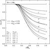 |
Fig. 17 Internal rotation laws Ω(r)/Ωo sketched with Eq. (12) and inferred for a 2.5 M⊙ test star at t/tMS = 0.36 and on the ZAMS, according to several parametrized values of the contrast parameter p adopted for t/tMS = 0.36 that all account for the observed rotational velocity at this evolutionary phase. For each parameter pt/tMS we obtained the corresponding pZAMS, so that for the same specific total angular momentum J/M the corresponding angular velocity ratio Ωo/Ωe can explain the observed rotational velocity vZAMS given in Table 8. |
6. Comments and conclusions
Paper III provides rotational velocity distributions for A-type star groups defined according to their spectral types. The derivation of fundamental parameters allowed us to disentangle the effects of mass and evolutionary stage in these distributions. In spite of this more refined classification, the striking features already observed in Paper III remain unchanged (Figs. 6 and 9): (i) the noticeable lack of slow rotators in the low-mass end, i.e. M ≲ 2.5 M⊙ (ii) the genuine bimodal distributions for the high-mass end (M ≳ 2.5 M⊙). Taking advantage of the results shown in Figs. 13–15, we can attempt to put forward the following comments on some properties of these distributions.
On the one hand, we saw in Figs. 14 and 15 that in intermediate and late A-type stars (1.6 ≲ M/M⊙ ≲ 2.5) the rotational velocities undergo an acceleration from t/tMS ≈ 0 to t/tMS ≈ 0.3–0.4 and then remain high for a fairly long time, which can certainly help to keep the fraction of slow rotators low during subsequent evolutionary stages up to the TAMS.
On the other hand, Fig. 15 shows that stars with masses 2.5 ≲ M/M⊙ ≲ 3.5 also accelerate their surface rotation in the time interval ranging from t/tMS ≈ 0 to t/tMS ≈ 0.3, but undergo an efficient deceleration up to the TAMS, which we already commented in Sects. 5.2 and 5.3. We could then think of an initial, more or less genuine, bimodal distribution of rotational velocities among stars with masses in the 2.5 ≲ M/M⊙ ≲ 3 interval. The commented deceleration of rotational velocities can help to renew the population of slowly rotating stars as the evolution proceeds.
We conclude, however, that we have no substantial evidence to say why stars in the low-mass interval are more or less systematically not subject to efficient enough decelerating mechanisms that enable them to start their MS evolutionary phase with fairly high rotational velocities. In the same way the fraction of ZAMS slow rotators remains unexplained as well. We can guess, nevertheless, at two possibilities: (i) some stars in the present high-mass interval could start their MS phase after having completely exhausted their angular momentum in the pre-MS phase through magnetic braking, since it is difficult to believe that they never had any angular momentum (Tassoul 1978); (ii) there could be a fraction of undetected binaries where the tidal braking could have some effect. A systematic search of the fraction of rapidly rotating stars among those with small vsini parameters could perhaps shed new light on this question.
We have studied the evolution of the ratio of average true rotational velocities ⟨ v/vcrit ⟩ (v is the true equatorial velocity; vcrit is the critical equatorial velocity) of MS stars with masses ranging from 1.7 M⊙ to 3.3 M⊙. Using 2D models of rotating stars we calculated the vcrit for individual masses and ages, and obtained the evolution of the average true equatorial velocity ⟨ v ⟩ for three stellar masses: 2, 2.5 and 3 M⊙ plotted in Figs. 14 and 15. These masses summarize the main characteristics of the evolution of rotational velocities in the MS of stars in the 1.7 ≤ M/M⊙ ≤ 3.3 mass range.
The observed evolution of rotational velocities strongly differs from that theoretically predicted for two limiting cases of internal angular momentum redistribution: (i) rigid rotation (total redistribution); (ii) conservation of the specific angular momentum by each stellar shell (no redistribution). For all studied masses, the observed trends suggest that some effective mechanism of angular momentum redistribution favors the acceleration of the rotation in the stellar surface during the first third of the MS phase. This also makes stars in the studied mass-range possibly behave as differential rotators during all their MS phase. After the acceleration in the first third of the MS phase, stars with masses M = 2 M⊙ evolve with little change of their equatorial rotational velocity in the second third of the MS. In the last third of the MS, the rotational velocities decelerate because they were conserving the specific angular momentum per shell without any redistribution. Stars with masses M ≥ 2.5 M⊙ seem to have an efficient deceleration of the surface rotation during the second third of the MS, which is faster than imposed by a regime of no redistribution of angular momentum. A new acceleration of the surface rotational velocity seems to happen in the 0.6 ≲ t/tMS ≲ 0.7 time interval, but it decelerates again in the last third of the MS phase. This might be caused by some redistribution of angular momentum toward the center of stars, since according to their low mass-loss rates they cannot undergo strong losses of angular momentum. The variation of the surface rotational velocities proceeds at characteristic time scales that are mass-dependent, i.e. δt ≈ 0.2 tMS.
The comparison of the observed evolution of rotational velocities for stars with M = 3 M⊙ with that predicted by detailed calculations of redistribution processes in the stellar interiors shown in Fig. 16 reveals very strong deviations between theory and observations in the first half of the MS evolutionary phase. We note that a more pronounced spin-down trend during the second part of the MS compared with the M = 3 M⊙ model from Ekström et al. (2008) is found by HGM. According to the present work, this faster spin-down seems to be present in the last third of the MS, as shown in Fig. 16b.
From the total specific angular momentum calculated to account for the observed velocities of stars in different evolutionary stages if they were rigid rotators, we conclude that stars of all masses studied here could start the MS evolutionary phase with a lower total angular momentum than the limiting value ascribed to critical rigid rotators on the ZAMS. Also, the observed behavior of the equatorial velocities suggests that they evolve during most of the MS phase as simple differential rotators. However, the angular momenta obtained for masses M ≥ 2.5 M⊙ in their last third of the MS phase suggest that they must have larger amounts of rotational energy than rigid critical rotators can bear in the TAMS. This indicates that by the end of the MS they evolve as neat differential rotators.
Using a test star with M = 2.5 M⊙, we have speculated on the properties that its internal rotation may have on the ZAMS, if at this stage the surface rotational velocity corresponded to the total angular momentum required at t/tMS = 0.36, which is the highest estimated for stars of this mass and in particular, it is higher than the expected one on the ZAMS behaving as rigid rotator. We conclude that an angular velocity ratio Ωo/Ωe up to 1.3 on the ZAMS could be expected. Assuming that the 2.5 M⊙ test star is a simple differential rotator ( ), its equatorial velocity can correspond to angular velocity ratios Ωo/Ωe as high as 2.6 on the ZAMS, so that Ωo/Ωe ≲ 2.1 for p = 0.6 at t/tMS = 0.36. If the object were a neat differential rotator (
 ), stable Ωo/Ωe ratios up to 8.8 could exist on the ZAMS and up to 7 at t/tMS = 0.36.
The present discussion assumes that the internal rotation of stars has a shellular-like distribution. We noted in Paper III, however, that some A-type stars could present a radiative/convective structural dichotomy that could induce other types of angular velocity laws in the external layers and could accordingly affect the interpretation of the measured rotational velocities. This dichotomy might be responsible for anomalous von Zeipel coefficients in fast rotating A-type stars (Zhao et al. 2009). Fast rotation can, in particular, affect the temperature gradient in the stellar envelopes, producing thus enlarged convective zones in a similar way as was suggested for massive fast rotators (Maeder et al. 2008). Convection and rotation may then be coupled somehow to induce other rotational laws than of mere shellular type (Zorec et al. 2011a,b). In the future, tests should then be made to see which internal rotation profiles can actually prevail. These tests could perhaps be carried out by studying the non-radial pulsation modes of early A-type stars.
Online material
Appendix A: Models of rigid rotators
Only the general dynamical aspects induced by rotation were considered here to calculate the mass distribution in a star and consequently the gravitational potential of a centrifugally distorted star. We separated the primary dynamical effects produced by rotation from those induced by evolution. The primary thermodynamic effects carried by the stellar evolution were taken into account using barotropic relations calculated with stellar models without rotation. We assumed therefore that the changes produced in the P = P(ρ) relation at a given evolutionary stage of a star by the several instabilities and the diffusion of chemical elements unleashed through the stellar evolution by rotation have second-order effects on the establishment of the dynamical equilibrium of the rotating star. In principle, one could use the barotropic relations derived with models of stellar evolution with shellular rotation, but the results will not be more reliable. This approach is used and discussed recently by Zorec et al. (2011b) for massive and intermediate-mass fast rotating stars.
Because we are not interested in the precise description of all non-linear time-dependent phenomena associated with the viscosity and with internal flows in rotating stars, and because the total energy carried by the meridional circulation is low, our models are axisymmetric, steady state and circulation free. Because of these assumptions, our model-stars behave as barotropes (Poincaré-Wavre theorem Tassoul 1978). We adopted internal rotational laws of conservative form, Ω = Ω(ϖ), where ϖ is the distance to the rotation axis. The rigid rotation is a special case of this type of rotational laws. In this case, the gravitational potential Φ(ϖ,z) and the density distribution ρ(ϖ,z) in the rotating star are simultaneous solutions to the hydrostatic equilibrium equation:  (A.1)and to the Poisson equation
  (A.2)where (ϖ,φ,z) are the cylindrical coordinates with z containing the rotation axis; êϖ is the unit vector perpendicular to the z-axis; P is the pressure; j = Ωϖ2 is the specific angular momentum.
Equations (A.1) and (A.2) are solved with the adopted complementary barotropic relation  (A.3)where the constants a, b, γa and γb were adjusted to (i) reproduce the pressure Pc and the density ρc in the center of the non-rotating star of given mass and evolutionary stage; (ii) ensure a continuous distribution of the pressure-density relation at the radius of the stellar core; (iii) obtain the right stellar mass at the stellar radius as tabulated by Schaller et al. (1992) for 1D evolutionary models for the initial metallicity Z = 0.02. The function (A.3) is continued in the stellar atmosphere by another pressure-density relation calculated by Castelli & Kurucz (2003) for stellar atmospheres as a function of the parameters (Teff,log g).
The first-order effects from the stellar evolution are thus accounted for by the pressure-density relations in the center of the star and by the ∂P/∂ρ gradients. An additional term in relation (A.3) could in principle also take into account the presence of the convective regions in the envelope induced by fast rotation, but we did not do this here. The only rotational effect considered here on the P = P(ρ) relation is through the mass-compensation effect (Sackmann 1970), which increases the density ρc in the center of the star. For this, we iterated ρc until the nominal stellar mass M was obtained. This iteration also implies that the central pressure Pc changes in accordance.
The gravitational potential Φ(ϖ,z) was obtained by solving Poisson equation (A.2) with the cell-method adapted by Clement (1974) for stellar structure calculations. The density distribution ρ(ϖ,z) was derived through the integrated form of (A.1).
Given an angular rotational velocity Ω and a barotropic relation (A.3), the solutions of Eqs. (A.1) and (A.2) were performed over the entire space. The iteration of Φ and ρ was stopped when the highest density difference in the (ϖ,z)-space is max(δρ/ρ) ≲ 10-6. In our iterations the virial relation δ = [2(K + U) − W]/| W| = 0 (K = kinetic energy; U = internal energy; W = total gravitational potential energy) is verified to better than δ ≈ 2 × 10⁻⁴ in the ZAMS models and δ ≈ 6 × 10⁻³ by the TAMS models. Since in the frame of conservative rotational laws the surfaces of constant pressure, density, and of total potential are parallel, the rotationally distorted shape of our models is defined by the total equipotential surface that contains the polar “photospheric” radius Rp. This radius is identified by the layer whose density satisfies the model-atmosphere relation τRoss(ρ) = 2/3 in the stellar atmosphere models of Castelli & Kurucz (2003). The local effective temperature at the pole needs to also satisfy the gravity darkening effect. We accordingly modified the effective temperature given by Schaller et al. (1992) for the given mass M using von Zeipel’s approximation (von Zeipel 1924). The transformation to the rotation dependent effective temperature was performed following the procedure given in Frémat et al. (2005).
The models calculated in this work are for specific total angular momentum scaled as J/M = 0.1, 1/3, 2/3 and  , where
  is the critical value supported by the stars on the TAMS. We also assumed that the stars evolve conserving their initial angular momentum. The velocity ratios for J/M = 0 and
  are plotted in Fig. 10. The characteristic parameters of the models calculated are given in Table B.1.
Appendix B: Models of differential rotators
The angular velocity distribution Ω′(r′) at time t′ can be derived at time t if we obtain the relation r′ = r′(r) that describes the change of the radius r of a shell at time t to the radius r′ of the same shell at time t′. This can be done observing that the mass inside a given radius r at time t must be the same as that inside r′ at time t′:  (B.1)A similar relation can be obtained from (7) by imposing that the angular momentum inside r at time t is the same as inside r′ at the time t′. This relation is much more difficult to manage, however, since the distribution of the angular velocity Ω(x′) and t′ must be iterated. In Fig. B.1 we show the internal rotational profiles at different evolutionary phases identified by the ratios t/tMS, where t is the stellar age from the ZAMS and tMS is the stellar age on the TAMS. These distributions were obtained assuming that on the ZAMS the star is a rigid rotator. In Fig. B.1 the angular velocities are normalized to the angular velocity at r = 0. The shaded region corresponds to the extent of the stellar core. We note that in current models of massive and intermediate-mass rotating stars, it is assumed that in the convective core Ωcore = const. In that case a distribution like the one sketched for t/tMS = 0.247 is expected.
To include the effect of the internal rotation on the stellar moment of inertia and on the stellar radius, we used the angular velocities shown in Fig. B.1 that are interpreted as conservative, i.e. written as a function of the distance ϖ to the rotational axis. Since the total rotational energy is low, i.e. J/M ≤ (J/M)crit, differences in the estimation of stellar radii are small as noted by the loci of points in Fig. 10 for J/M = 0 and J/M = (J/M)crit.
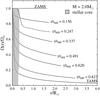 |
Fig. B.1 Internal angular velocity at different evolutionary stages in MS for a 2 M⊙ rigidly rotating star on the ZAMS that evolves without any exchange of the angular momentum among the stellar shells. The shaded zone represents the stellar core, where the current models with rotation assume that it rotates rigidly. In this case, the internal angular velocity is redistributed as sketched for the t/tMS = 0.247 phase. |
Parameters characterizing the models of rigid rotators that evolve with constant angular momentum  , with
  for rigid rotation.
This smoothing parameter is larger than the estimation using the definition by Sheather & Jones (1991), made in Paper III. This is the reason why the distributions are smoother (Silverman 1986). This smoothing parameter has been used in the different parts of the study, both in one and two dimensions (see Sect. 5.2).
The lag parameter ℓ allows us to shift the Maxwellian distribution along the x-axis:  .
.
Acknowledgments
We are thankful to an anonymous referee for her/his valuable comments and suggestions that helped to improve the presentation of our results. We are also very grateful to Prof. Hugo Levato for the communication of his data. This work has widely made use of the CDS database.
References
- Abt, H. A. 2009, AJ, 138, 28 [NASA ADS] [CrossRef] [Google Scholar]
- Abt, H. A., & Morrell, N. I. 1995, ApJS, 99, 135 [Google Scholar]
- Abt, H. A., Levato, H., & Grosso, M. 2002, ApJ, 573, 359 (ALG) [NASA ADS] [CrossRef] [Google Scholar]
- Attridge, J. M., & Herbst, W. 1992, ApJ, 398, L61 [NASA ADS] [CrossRef] [Google Scholar]
- Barnes, S. A. 2003, ApJ, 586, L145 [NASA ADS] [CrossRef] [Google Scholar]
- Bodenheimer, P. 1981, in Fundamental Problems in the Theory of Stellar Evolution (Dordrecht: D. Reidel Publishing Co.), IAU Symp., 93, 5 [Google Scholar]
- Bowman, A. W., & Azzalini, A. 1997, Applied smoothing techniques for data analysis: the kernel approach with S-plus illustrations, Oxford statistical science series No. 18 (Oxford: Clarendon Press) [Google Scholar]
- Castelli, F. 1991, A&A, 251, 106 [NASA ADS] [Google Scholar]
- Castelli, F., & Kurucz, R. L. 2003, in Modelling of Stellar Atmospheres, ed. N. Piskunov, W. W. Weiss, & D. F. Gray (San Francisco: ASP), IAU Symp., 210, 20P [Google Scholar]
- Chandrasekhar, S. 1969, Ellipsoidal figures of equilibrium, ed. S. Chandrasekhar (New Haven: Yale University Press) [Google Scholar]
- Chandrasekhar, S., & Münch, G. 1950, ApJ, 111, 142 [NASA ADS] [CrossRef] [MathSciNet] [Google Scholar]
- Choi, P. I., & Herbst, W. 1996, AJ, 111, 283 [NASA ADS] [CrossRef] [Google Scholar]
- Clement, M. J. 1974, ApJ, 194, 709 [NASA ADS] [CrossRef] [Google Scholar]
- Debernardi, Y. 2000, in Birth and Evolution of Binary Stars, ed. B. Reipurth, & H. Zinnecker (San Francisco: ASP), IAU Symp., 200, 161 [Google Scholar]
- Deutsch, A. J. 1970, in Stellar rotation, ed. A. Slettebak (Dordrecht: D. Reidel Publishing Co.), IAU Colloq., 4, 207 [Google Scholar]
- Díaz, C. G., González, J. F., Levato, H., & Grosso, M. 2011, A&A, 531, A143 [NASA ADS] [CrossRef] [EDP Sciences] [Google Scholar]
- Edwards, S., Strom, S. E., Hartigan, P., et al. 1993, AJ, 106, 372 [NASA ADS] [CrossRef] [Google Scholar]
- Ekström, S., Meynet, G., Maeder, A., & Barblan, F. 2008, A&A, 478, 467 [NASA ADS] [CrossRef] [EDP Sciences] [Google Scholar]
- Ekström, S., Georgy, C., Eggenberger, P., et al. 2011, A&A, in press, DOI: 10.1051/0004-6361/201117751 [Google Scholar]
- Endal, A. S., & Sofia, S. 1981, ApJ, 243, 625 [NASA ADS] [CrossRef] [Google Scholar]
- Erspamer, D., & North, P. 2003, A&A, 398, 1121 [NASA ADS] [CrossRef] [EDP Sciences] [Google Scholar]
- ESA 1997, The Hipparcos and Tycho Catalogues, ESA SP, 1200 [Google Scholar]
- Fekel, F. C. 2003, PASP, 115, 807 [NASA ADS] [CrossRef] [Google Scholar]
- Frémat, Y., & Zorec, J. 2003, in Modelling of Stellar Atmospheres, ed. N. Piskunov, W. W. Weiss, & D. F. Gray (San Francisco: ASP), IAU Symp., 210, 27 [Google Scholar]
- Frémat, Y., Zorec, J., Hubert, A. M., Floquet, M., & Cidale, L. 2003, in Modelling of Stellar Atmospheres, ed. N. Piskunov, W. W. Weiss, & D. F. Gray (San Francisco: ASP), IAU Symp., 210, 26 [Google Scholar]
- Frémat, Y., Zorec, J., Hubert, A.-M., & Floquet, M. 2005, A&A, 440, 305 [NASA ADS] [CrossRef] [EDP Sciences] [Google Scholar]
- Guthrie, B. N. G. 1982, MNRAS, 198, 795 [NASA ADS] [Google Scholar]
- Hauck, B., & Mermilliod, M. 1998, A&AS, 129, 431 [NASA ADS] [CrossRef] [EDP Sciences] [Google Scholar]
- Herbst, W., Bailer-Jones, C. A. L., & Mundt, R. 2001, ApJ, 554, L197 [NASA ADS] [CrossRef] [Google Scholar]
- Howarth, I. D. 2004, in Stellar Rotation, ed. A. Maeder, & P. Eenens (San Francisco: ASP), IAU Symp., 215, 33 [Google Scholar]
- Huang, W., Gies, D. R., & McSwain, M. V. 2010, ApJ, 722, 605 (HGM) [NASA ADS] [CrossRef] [Google Scholar]
- Hubrig, S., North, P., & Mathys, G. 2000, ApJ, 539, 352 [NASA ADS] [CrossRef] [Google Scholar]
- Jefferys, W. H., Fitzpatrick, M. J., & McArthur, B. E. 1998a, Celest. Mech., 41, 39 [Google Scholar]
- Jefferys, W. H., Fitzpatrick, M. J., McArthur, B. E., & McCartney, J. E. 1998b, GaussFit: A System for least squares and robust estimation, User’s Manual, Dept. of Astronomy and McDonald Observatory, Austin, Texas [Google Scholar]
- Keppens, R., MacGregor, K. B., & Charbonneau, P. 1995, A&A, 294, 469 [NASA ADS] [Google Scholar]
- Königl, A. 1991, ApJ, 370, L39 [NASA ADS] [CrossRef] [Google Scholar]
- Lamers, H. J. G. L. M., & Cassinelli, J. P. 1999, Introduction to Stellar Winds, ed. H. J. G. L. M. Lamers, & J. P. Cassinelli (Cambridge University Press) [Google Scholar]
- Landstreet, J. D., Bagnulo, S., Andretta, V., et al. 2007, A&A, 470, 685 [NASA ADS] [CrossRef] [EDP Sciences] [Google Scholar]
- Lang, K. R. 1992, Astrophysical Data I. Planets and Stars., ed. K. R. Lang (Berlin: Springer-Verlag) [Google Scholar]
- Lanz, T., & Catala, C. 1992, A&A, 257, 663 [NASA ADS] [Google Scholar]
- Latour, J., Toomre, J., & Zahn, J.-P. 1981, ApJ, 248, 1081 [Google Scholar]
- Levato, H., & Grosso, M. 2004, in Stellar Rotation, ed. A. Maeder, & P. Eenens (San Francisco: ASP), IAU Symp., 215, 51 (LG) [Google Scholar]
- Lucy, L. B. 1974, AJ, 79, 745 [NASA ADS] [CrossRef] [Google Scholar]
- MacGregor, K. B., & Brenner, M. 1991, ApJ, 376, 204 [NASA ADS] [CrossRef] [Google Scholar]
- Maeder, A., & Meynet, G. 2000, ARA&A, 38, 143 [NASA ADS] [CrossRef] [Google Scholar]
- Maeder, A., Georgy, C., & Meynet, G. 2008, A&A, 479, L37 [NASA ADS] [CrossRef] [EDP Sciences] [Google Scholar]
- Matsumoto, T., Hanawa, T., & Nakamura, F. 1997, ApJ, 478, 569 [NASA ADS] [CrossRef] [Google Scholar]
- Moon, T. T., & Dworetsky, M. M. 1985, MNRAS, 217, 305 [NASA ADS] [CrossRef] [Google Scholar]
- Mouschovias, T. C., & Morton, S. A. 1985a, ApJ, 298, 205 [NASA ADS] [CrossRef] [Google Scholar]
- Mouschovias, T. C., & Morton, S. A. 1985b, ApJ, 298, 190 [NASA ADS] [CrossRef] [Google Scholar]
- Napiwotzki, R., Schoenberner, D., & Wenske, V. 1993, A&A, 268, 653 [NASA ADS] [Google Scholar]
- Pinsonneault, M. H., Kawaler, S. D., & Demarque, P. 1990, ApJS, 74, 501 [NASA ADS] [CrossRef] [Google Scholar]
- Pourbaix, D., Tokovinin, A. A., Batten, A. H., et al. 2004, A&A, 424, 727 [NASA ADS] [CrossRef] [EDP Sciences] [Google Scholar]
- Pudritz, R. E. 1985, ApJ, 293, 216 [NASA ADS] [CrossRef] [Google Scholar]
- Reiners, A., & Royer, F. 2004, A&A, 415, 325 [Google Scholar]
- Renson, P., & Manfroid, J. 2009, A&A, 498, 961 [NASA ADS] [CrossRef] [EDP Sciences] [Google Scholar]
- Richardson, W. H. 1972, J. Opt. Soc. Am., 62, 55 [Google Scholar]
- Royer, F. 2009, in The Rotation of Sun and Stars, ed. J.-P. Rozelot, & C. Neiner (Berlin: Springer Verlag), Lect. Notes Phys., 765, 207 [Google Scholar]
- Royer, F., Gerbaldi, M., Faraggiana, R., & Gómez, A. E. 2002a, A&A, 381, 105 (Paper I) [NASA ADS] [CrossRef] [EDP Sciences] [Google Scholar]
- Royer, F., Grenier, S., Baylac, M.-O., Gómez, A. E., & Zorec, J. 2002b, A&A, 393, 897 (Paper II) [NASA ADS] [CrossRef] [EDP Sciences] [Google Scholar]
- Royer, F., Zorec, J., & Gómez, A. E. 2007, A&A, 463, 671 (Paper III) [NASA ADS] [CrossRef] [EDP Sciences] [Google Scholar]
- Sackmann, I. J. 1970, A&A, 8, 76 [NASA ADS] [Google Scholar]
- Schaller, G., Schaerer, D., Meynet, G., & Maeder, A. 1992, A&AS, 96, 269 [Google Scholar]
- Schatzman, E. 1962, Ann. Ap., 25, 18 [Google Scholar]
- Sheather, S. J., & Jones, M. C. 1991, J. R. Statist. Soc. B, 53, 683 [Google Scholar]
- Shu, F. H., Najita, J. R., Shang, H., & Li, Z.-Y. 2000, in Protostars and Planets IV, ed. V. Mannings, A. P. Boss, & S. S. Russell (Tucson: University of Arizona Press), 789 [Google Scholar]
- Silverman, B. W. 1986, Density estimation for statistics and data analysis, Monographs on Statistics and Applied Probability No. 26 (London: Chapman & Hall) [Google Scholar]
- Slettebak, A., Collins, I. G. W., Boyce, P. B., White, N. M., & Parkinson, T. D. 1975, ApJS, 29, 137 [NASA ADS] [CrossRef] [Google Scholar]
- Soderblom, D. R., Stauffer, J. R., MacGregor, K. B., & Jones, B. F. 1993, ApJ, 409, 624 [NASA ADS] [CrossRef] [Google Scholar]
- Soderblom, D. R., Jones, B. F., & Fischer, D. 2001, ApJ, 563, 334 [NASA ADS] [CrossRef] [Google Scholar]
- Spruit, H. C. 1999, A&A, 349, 189 [NASA ADS] [Google Scholar]
- Spruit, H. C. 2002, A&A, 381, 923 [NASA ADS] [CrossRef] [EDP Sciences] [Google Scholar]
- Stauffer, J. R., Hartmann, L., Soderblom, D. R., & Burnham, N. 1984, ApJ, 280, 202 [NASA ADS] [CrossRef] [Google Scholar]
- Stȩpień, K. 2000, A&A, 353, 227 [NASA ADS] [Google Scholar]
- Tassoul, J.-L. 1978, Theory of rotating stars (Princeton University Press) [Google Scholar]
- van Leeuwen, F. 2007, A&A, 474, 653 [NASA ADS] [CrossRef] [EDP Sciences] [Google Scholar]
- von Zeipel, H. 1924, MNRAS, 84, 665 [NASA ADS] [CrossRef] [Google Scholar]
- Zhao, M., Monnier, J. D., Pedretti, E., et al. 2009, ApJ, 701, 209 [NASA ADS] [CrossRef] [Google Scholar]
- Zorec, J., & Briot, D. 1997, A&A, 318, 443 [NASA ADS] [Google Scholar]
- Zorec, J., Frémat, Y., Hubert, A. M., Floquet, M., & Cidale, L. 2002, in Rev. Mex. Astron. Astrofis. Conf. Ser., ed. J. J. Claria, D. Garcia Lambas, & H. Levato, 14, 114 [Google Scholar]
- Zorec, J., Frémat, Y., & Cidale, L. 2005, A&A, 441, 235 [NASA ADS] [CrossRef] [EDP Sciences] [Google Scholar]
- Zorec, J., Frémat, Y., & Domiciano de Souza, A. 2007, in Active OB-Stars: Laboratories for Stellar and Circumstellar Physics, ed. A. T. Okazaki, S. P. Owocki, & S. Štefl (San Francisco: ASP), ASP Conf. Ser., 361, 542 [Google Scholar]
- Zorec, J., Cidale, L., Arias, M. L., et al. 2009, A&A, 501, 297 [NASA ADS] [CrossRef] [EDP Sciences] [Google Scholar]
- Zorec, J., Frémat, Y., Delaa, O., et al. 2011a, in Active OB stars: structure, evolution, mass loss, and critical limits, ed. C. Neiner, G. Wade, G. Meynet, & G. Peters (Cambridge University Press), IAU Symp. 272, 103 [Google Scholar]
- Zorec, J., Frémat, Y., Domiciano de Souza, A., et al. 2011b, A&A, 526, A87 [NASA ADS] [CrossRef] [EDP Sciences] [Google Scholar]
All Tables
List of the 2014 B6- to F2-type stars, with their spectral type and fundamental parameters (extract).
Mass and age estimates using evolutionary tracks with rotation for a test star with apparent rotation-less mass M = 3 M⊙.
Parameters of the 1D velocity distributions for normal stars as a function of the stellar mass.
Parameters of the 1D velocity distributions for all stars (normal, CP and CB) as a function of the stellar mass.
Synopsis of the average evolution of equatorial velocities of 2 M⊙, 2.5 M⊙ and 3 M⊙ stars.
Contrast parameters p, angular velocity ratios Ωo/Ωe and total specific angular momenta J/M in a 2.5 M⊙ test star.
Parameters characterizing the models of rigid rotators that evolve with constant angular momentum , with for rigid rotation.
All Figures
|
Fig. 1 Comparison of vsini data: a) values for the 94 stars (with spectral type equal to, or later than, B6) in common between Abt et al. (2002) and Levato & Grosso (2004). The dashed line stands for the one-to-one relation and the solid line is the result from Eq. (1); b) values for the 199 stars (with spectral type equal to, or later than, B6) in common between merged data from Abt et al. (2002) and Levato & Grosso (2004), and Royer et al. (2002b). The solid line is the result from Eq. (2); c) values for the 44 stars (with spectral type equal to, or later than, B6) in common between Huang et al. (2010) and previously merged data. The solid line is the result from Eq. (3). |
| In the text | |
|
Fig. 2 Color-effective temperature diagram for the single normal stars selected for the present study. |
| In the text | |
|
Fig. 3 Comparison of effective temperatures calculated in this paper from the uvby − β photometry and those for 135 stars obtained using bolometric fluxes. The dashed line is the one-to-one relation. |
| In the text | |
|
Fig. 4 HR diagram of the studied stars. Only the single normal stars in the shaded region were selected for the present study. Filled circles are for stars in the sample studied by Royer et al. (2007). Open circles, open diamonds and asterisks stand for complementary stars taken from Abt et al. (2002), Levato & Grosso (2004) and Huang et al. (2010) respectively. The evolutionary tracks are from Schaller et al. (1992). |
| In the text | |
|
Fig. 5 Distribution in the (t/tMS,M/M⊙) plane of the data concerning the single normal stars selected for the present study. The error bars in both coordinates are indicated in gray. The symbols have the same meaning as in Fig. 4. |
| In the text | |
|
Fig. 6 Distributions of rotational velocities for normal stars in different mass subsamples: shaded histograms are the observed vsini; solid thick lines are the distributions of equatorial velocities and the gray strips are their associated variability bands. The dashed lines stand for the Maxwellian fit, whose parameters are given in Table 4. The mass range for each subsample is indicated in the corresponding panel, together with the number of stars. The histograms are normalized to fit the probability density scale. |
| In the text | |
|
Fig. 7 Distribution of true rotational velocities v for normal stars as a function of the stellar mass M/M⊙. The color scale represents the density in the one-dimensional normalized distributions. The bluer the region, the smaller the number of stars and vice versa for the red colored scale. White solid lines follow iso-density contours. |
| In the text | |
|
Fig. 8 Mean age ⟨ t/tMS ⟩ per bin of vsini for different mass intervals (taken from Table 4): a) 2 < M/M⊙ < 2.4; b) 2.2 < M/M⊙ < 2.6; c) 2.35 < M/M⊙ < 2.85; d) 2.55 < M/M⊙ < 3.05. Filled circles stand for normal stars, whereas open squares represent CP stars. The bins in vsini are 40 km s-1 wide. Solid lines are the results of linear fits on normal stars with vsini ≤ 110 km s-1 and dashed lines the results of the fits for CP stars with vsini ≥ 90 km s-1. |
| In the text | |
|
Fig. 9 Distributions of rotational velocities as a function of age for two mass subsamples. Left panels correspond to the low-mass bin: 1.6–2.4 M⊙ and right panels correspond to the high-mass bin: 2.4–3.85 M⊙. As in Fig. 6, shaded histograms are the observed vsini; solid thick lines are the distributions of equatorial velocities v and the gray strips are their associated variability bands. The mass range for each subsample is indicated in the corresponding panel together with the number of stars, and below, the age interval is indicated and goes from young stars (0 < t/tMS < 0.5) in upper panels to stars close to the TAMS (0.8 < t/tMS < 1) in lower panels. The histograms are normalized to fit the probability density scale. |
| In the text | |
|
Fig. 10 v/vZAMS ratio of equatorial rotational velocities as a function of the t/tMS time ratio in the MS for stars with masses from M = 1.5 to 3 M⊙. vZAMS is the equatorial rotational velocity on the ZAMS, t is the stellar age and tMS is the time that a star of given mass M can remain in the MS. Two extreme cases are represented: stars evolving as rigid rotators (instantaneous complete angular momentum redistribution) and as differential rotators without any angular momentum redistribution. Dashed lines represent the limits for J/M → 0, while the solid lines are for stars that on the ZAMS have a specific angular momentum that in the TAMS becomes the critical one. |
| In the text | |
|
Fig. 11 Theoretical evolution of the v/vcrit velocity ratio calculated for several stellar masses. a) Dependence with time of the v/vcrit ratio for several values of the total specific angular momentum J, when stars evolve as rigid rotators all long the MS phase; b) evolution of the ratio v/vcrit normalized to its value on the ZAMS when rotators conserve the angular momentum by shells. |
| In the text | |
|
Fig. 12 Critical equatorial rotational velocities of stars with different masses as a function of age in the MS. At each t/tMS the objects are assumed to be rigid rotators. |
| In the text | |
|
Fig. 13 Distribution of the ratio v/vcrit of true rotational velocities as a function of the fractional age in the MS evolutionary phase for normal stars in the mass interval 1.7 ≤ M ≤ 3.3 M⊙. The filled circles are the average positions of the stars in running boxes with bins of 0.15 in t/tMS and 0.5 in M/M⊙. |
| In the text | |
|
Fig. 14 Evolution of the equatorial velocity ratio ⟨ v/vcrit ⟩ in the MS life time span. The ratios of true equatorial velocities are calculated for three masses: 2 M⊙, 2.5 M⊙ and 3 M⊙. The shaded regions correspond to the theoretical evolution of the v/vcrit ratio in rigid rotators plotted in Fig. 11, whose total angular momenta are |
| In the text | |
|
Fig. 15 Evolution of the equatorial velocity ratio ⟨ v/vZAMS ⟩ in the MS life time span, where vZAMS is the true equatorial velocity of stars on the ZAMS. The average true equatorial velocities were calculated for the same masses as in Fig. 14. The shaded regions correspond to the theoretical evolution of the v/vZAMS ratios shown in Fig. 10: rigid rotators (middle), simple differential rotators (lower left corner). |
| In the text | |
|
Fig. 16 Comparison of the observed evolution of equatorial velocity ratios in the MS life time span for stars with M = 3 M⊙ inferred from observations with theoretical ones calculated by Ekström et al. (2008) for different v/vcrit on the ZAMS. a) Evolution of ⟨ v/vcrit ⟩ ratios; b) evolution of ⟨ v/vZAMS ⟩ ratios. |
| In the text | |
|
Fig. 17 Internal rotation laws Ω(r)/Ωo sketched with Eq. (12) and inferred for a 2.5 M⊙ test star at t/tMS = 0.36 and on the ZAMS, according to several parametrized values of the contrast parameter p adopted for t/tMS = 0.36 that all account for the observed rotational velocity at this evolutionary phase. For each parameter pt/tMS we obtained the corresponding pZAMS, so that for the same specific total angular momentum J/M the corresponding angular velocity ratio Ωo/Ωe can explain the observed rotational velocity vZAMS given in Table 8. |
| In the text | |
|
Fig. B.1 Internal angular velocity at different evolutionary stages in MS for a 2 M⊙ rigidly rotating star on the ZAMS that evolves without any exchange of the angular momentum among the stellar shells. The shaded zone represents the stellar core, where the current models with rotation assume that it rotates rigidly. In this case, the internal angular velocity is redistributed as sketched for the t/tMS = 0.247 phase. |
| In the text | |
Current usage metrics show cumulative count of Article Views (full-text article views including HTML views, PDF and ePub downloads, according to the available data) and Abstracts Views on Vision4Press platform.
Data correspond to usage on the plateform after 2015. The current usage metrics is available 48-96 hours after online publication and is updated daily on week days.
Initial download of the metrics may take a while.