| Issue |
A&A
Volume 537, January 2012
|
|
|---|---|---|
| Article Number | A120 | |
| Number of page(s) | 22 | |
| Section | Stellar structure and evolution | |
| DOI | https://doi.org/10.1051/0004-6361/201117691 | |
| Published online | 19 January 2012 | |
Online material
Appendix A: Models of rigid rotators
Only the general dynamical aspects induced by rotation were considered here to calculate the mass distribution in a star and consequently the gravitational potential of a centrifugally distorted star. We separated the primary dynamical effects produced by rotation from those induced by evolution. The primary thermodynamic effects carried by the stellar evolution were taken into account using barotropic relations calculated with stellar models without rotation. We assumed therefore that the changes produced in the P = P(ρ) relation at a given evolutionary stage of a star by the several instabilities and the diffusion of chemical elements unleashed through the stellar evolution by rotation have second-order effects on the establishment of the dynamical equilibrium of the rotating star. In principle, one could use the barotropic relations derived with models of stellar evolution with shellular rotation, but the results will not be more reliable. This approach is used and discussed recently by Zorec et al. (2011b) for massive and intermediate-mass fast rotating stars.
Because we are not interested in the precise description of all non-linear time-dependent phenomena associated with the viscosity and with internal flows in rotating stars, and because the total energy carried by the meridional circulation is low, our models are axisymmetric, steady state and circulation free. Because of these assumptions, our model-stars behave as barotropes (Poincaré-Wavre theorem Tassoul 1978). We adopted internal rotational laws of conservative form, Ω = Ω(ϖ), where ϖ is the distance to the rotation axis. The rigid rotation is a special case of this type of rotational laws. In this case, the gravitational potential Φ(ϖ,z) and the density distribution ρ(ϖ,z) in the rotating star are simultaneous solutions to the hydrostatic equilibrium equation: 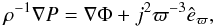 (A.1)and to the Poisson equation
  (A.2)where (ϖ,φ,z) are the cylindrical coordinates with z containing the rotation axis; êϖ is the unit vector perpendicular to the z-axis; P is the pressure; j = Ωϖ2 is the specific angular momentum.
Equations (A.1) and (A.2) are solved with the adopted complementary barotropic relation  (A.3)where the constants a, b, γa and γb were adjusted to (i) reproduce the pressure Pc and the density ρc in the center of the non-rotating star of given mass and evolutionary stage; (ii) ensure a continuous distribution of the pressure-density relation at the radius of the stellar core; (iii) obtain the right stellar mass at the stellar radius as tabulated by Schaller et al. (1992) for 1D evolutionary models for the initial metallicity Z = 0.02. The function (A.3) is continued in the stellar atmosphere by another pressure-density relation calculated by Castelli & Kurucz (2003) for stellar atmospheres as a function of the parameters (Teff,log g).
The first-order effects from the stellar evolution are thus accounted for by the pressure-density relations in the center of the star and by the ∂P/∂ρ gradients. An additional term in relation (A.3) could in principle also take into account the presence of the convective regions in the envelope induced by fast rotation, but we did not do this here. The only rotational effect considered here on the P = P(ρ) relation is through the mass-compensation effect (Sackmann 1970), which increases the density ρc in the center of the star. For this, we iterated ρc until the nominal stellar mass M was obtained. This iteration also implies that the central pressure Pc changes in accordance.
The gravitational potential Φ(ϖ,z) was obtained by solving Poisson equation (A.2) with the cell-method adapted by Clement (1974) for stellar structure calculations. The density distribution ρ(ϖ,z) was derived through the integrated form of (A.1).
Given an angular rotational velocity Ω and a barotropic relation (A.3), the solutions of Eqs. (A.1) and (A.2) were performed over the entire space. The iteration of Φ and ρ was stopped when the highest density difference in the (ϖ,z)-space is max(δρ/ρ) ≲ 10-6. In our iterations the virial relation δ = [2(K + U) − W]/| W| = 0 (K = kinetic energy; U = internal energy; W = total gravitational potential energy) is verified to better than δ ≈ 2 × 10⁻⁴ in the ZAMS models and δ ≈ 6 × 10⁻³ by the TAMS models. Since in the frame of conservative rotational laws the surfaces of constant pressure, density, and of total potential are parallel, the rotationally distorted shape of our models is defined by the total equipotential surface that contains the polar “photospheric” radius Rp. This radius is identified by the layer whose density satisfies the model-atmosphere relation τRoss(ρ) = 2/3 in the stellar atmosphere models of Castelli & Kurucz (2003). The local effective temperature at the pole needs to also satisfy the gravity darkening effect. We accordingly modified the effective temperature given by Schaller et al. (1992) for the given mass M using von Zeipel’s approximation (von Zeipel 1924). The transformation to the rotation dependent effective temperature was performed following the procedure given in Frémat et al. (2005).
The models calculated in this work are for specific total angular momentum scaled as J/M = 0.1, 1/3, 2/3 and  , where
  is the critical value supported by the stars on the TAMS. We also assumed that the stars evolve conserving their initial angular momentum. The velocity ratios for J/M = 0 and
  are plotted in Fig. 10. The characteristic parameters of the models calculated are given in Table B.1.
Appendix B: Models of differential rotators
The angular velocity distribution Ω′(r′) at time t′ can be derived at time t if we obtain the relation r′ = r′(r) that describes the change of the radius r of a shell at time t to the radius r′ of the same shell at time t′. This can be done observing that the mass inside a given radius r at time t must be the same as that inside r′ at time t′: 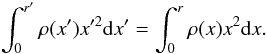 (B.1)A similar relation can be obtained from (7) by imposing that the angular momentum inside r at time t is the same as inside r′ at the time t′. This relation is much more difficult to manage, however, since the distribution of the angular velocity Ω(x′) and t′ must be iterated. In Fig. B.1 we show the internal rotational profiles at different evolutionary phases identified by the ratios t/tMS, where t is the stellar age from the ZAMS and tMS is the stellar age on the TAMS. These distributions were obtained assuming that on the ZAMS the star is a rigid rotator. In Fig. B.1 the angular velocities are normalized to the angular velocity at r = 0. The shaded region corresponds to the extent of the stellar core. We note that in current models of massive and intermediate-mass rotating stars, it is assumed that in the convective core Ωcore = const. In that case a distribution like the one sketched for t/tMS = 0.247 is expected.
To include the effect of the internal rotation on the stellar moment of inertia and on the stellar radius, we used the angular velocities shown in Fig. B.1 that are interpreted as conservative, i.e. written as a function of the distance ϖ to the rotational axis. Since the total rotational energy is low, i.e. J/M ≤ (J/M)crit, differences in the estimation of stellar radii are small as noted by the loci of points in Fig. 10 for J/M = 0 and J/M = (J/M)crit.
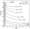 |
Fig. B.1
Internal angular velocity at different evolutionary stages in MS for a 2 M⊙ rigidly rotating star on the ZAMS that evolves without any exchange of the angular momentum among the stellar shells. The shaded zone represents the stellar core, where the current models with rotation assume that it rotates rigidly. In this case, the internal angular velocity is redistributed as sketched for the t/tMS = 0.247 phase. |
| Open with DEXTER | |
Parameters characterizing the models of rigid rotators that evolve with constant angular momentum  , with
  for rigid rotation.
© ESO, 2012
Current usage metrics show cumulative count of Article Views (full-text article views including HTML views, PDF and ePub downloads, according to the available data) and Abstracts Views on Vision4Press platform.
Data correspond to usage on the plateform after 2015. The current usage metrics is available 48-96 hours after online publication and is updated daily on week days.
Initial download of the metrics may take a while.