| Issue |
A&A
Volume 537, January 2012
|
|
|---|---|---|
| Article Number | A132 | |
| Number of page(s) | 21 | |
| Section | Stellar structure and evolution | |
| DOI | https://doi.org/10.1051/0004-6361/201117343 | |
| Published online | 23 January 2012 | |
A comparison between star formation rate diagnostics and rate of core collapse supernovae within 11 Mpc
1 INAF – Osservatorio Astronomico di Padova, Vicolo dell’Osservatorio 5, 35122 Padova, Italy
e-mail: This email address is being protected from spambots. You need JavaScript enabled to view it.
2 Astrophysics Research Centre, School of Mathematics and Physics, Queen’s University Belfast, Belfast BT7 1NN, UK
3 Institute of Astronomy, University of Cambridge, Madingley Road, Cambridge CB3 0HA, UK
4 Dipartimento di Fisica, Politecnico di Torino, Corso Duca degli Abruzzi 24, 10129 Torino, Italy
5 INFN, Sezione di Torino, via Pietro Giuria 1, 10125 Torino, Italy
6 Carnegie Fellow, Carnegie Observatories, 813 Santa Barbara Street, Pasadena, CA 91101, USA
Received: 25 May 2011
Accepted: 6 November 2011
Abstract
Aims. The core collapse supernova rate provides a strong lower limit for the star formation rate (SFR). Progress in using it as a cosmic SFR tracer requires some confidence that it is consistent with more conventional SFR diagnostics in the nearby Universe. This paper compares standard SFR measurements based on Hα, far ultraviolet (FUV) and total infrared (TIR) galaxy luminosities with the observed core collapse supernova rate in the same galaxy sample. The comparison can be viewed from two perspectives. Firstly, by adopting an estimate of the minimum stellar mass to produce a core collapse supernova one can determine a SFR from supernova numbers. Secondly, the radiative SFR can be assumed to be robust and then the supernova statistics provide a constrain on the minimum stellar mass for core collapse supernova progenitors.
Methods. The novel aspect of this study is that Hα, FUV and TIR luminosities are now available for a complete galaxy sample within the local 11 Mpc volume and the number of discovered supernovae in this sample within the last 13 years is high enough to perform a meaningful statistical comparison. We exploit the multi-wavelength dataset from 11 HUGS, a volume-limited survey designed to provide a census of SFR in the Local Volume. There are 14 supernovae discovered in this sample of galaxies within the last 13 years. Although one could argue that this may not be complete, it is certainly a robust lower limit.
Results. Assuming a lower limit for core collapse of 8 M⊙ (as proposed by direct detections of SN progenitor stars and white dwarf progenitors), the core-collapse supernova rate matches the SFR from the FUV luminosity. However, the SFR based on Hα luminosity is lower than these two estimates by a factor of nearly 2. If we assume that the FUV or Hα based luminosities are a true reflection of the SFR, we find that the minimum mass for core collapse supernova progenitors is 8 ± 1 M⊙ and 6 ± 1 M⊙, respectively.
Conclusions. The estimate of the minimum mass for core collapse supernova progenitors obtained exploiting FUV data is in good agreement with that from the direct detection of supernova progenitors. The concordant results by these independent methods point toward a constraint of 8 ± 1 M⊙ on the lower mass limit for progenitor stars of core collapse supernovae.
Key words: stars: massive / supernovae: general / galaxies: star formation
© ESO, 2012
1. Introduction
The progenitors of core collapse supernovae (CC SNe) are massive stars, either single or in binary systems, that complete exothermic nuclear burning, up to the development of an iron core that cannot be supported by any further nuclear fusion reactions or by electron degeneracy pressure. The subsequent collapse of the iron core results in the formation of a compact object, a neutron star or a black hole, accompanied by the high-velocity ejection of a large fraction of the progenitor mass. The SNe ejecta sweep, compress and heat the interstellar medium, and release the heavy elements which are produced during the progenitor evolution and in the explosion itself. This can further trigger subsequent star formation process (e.g. McKee & Ostriker 1977), hence having a profound effect on galaxy evolution.
Due to the short lifetime of their progenitor stars, the rate of occurrence of CC SNe closely follows the current star formation rate (SFR) in a stellar system. The evolution of the CC SN rate with redshift is a probe of the SF history (SFH) and allows us to constrain the chemical enrichment of the galaxies and the effect of energy/momentum feedback. Poor statistics is a major limiting factor for using the CC SN rate as a tracer of the SFR. At low redshift the difficulty is in sampling large enough volumes of the local universe to ensure significant statistics (e.g. Kennicutt 1984). While at high redshift the difficulty lies in detecting and typing complete samples of intrinsically faint SNe (Botticella et al. 2008; Bazin et al. 2009; Li et al. 2011a). Moreover some fraction of CC SNe are missed by optical searches, since they are embedded in dusty spiral arms or galaxy nuclei. This fraction may change with redshift, if the amount of dust in galaxies evolves with time. Progress in using CC SN rates as SFR tracers requires accurate measurements of rates at various cosmic epochs and in different environments. Furthermore it requires a meaningful comparison with other SFR diagnostics to verify its reliability and to analyse its main limitations.
The CC SN rate is also a powerful tool to investigate the nature of SN progenitor stars and to test stellar evolutionary models. Different sub-types of CC SNe have been identified on the basis of their spectroscopic and photometric properties and a possible sequence has been proposed on the basis of the progenitor mass loss history with the most massive stars losing the largest fraction of their initial mass (Heger et al. 2003). However, this simple scheme where only the mass loss drives the evolution of massive stars cannot easily explain the variety of observational properties showed by CC SNe of the same sub-type and the relative numbers of different sub-types (Smartt 2009).
In particular, two important outstanding issues are: the minimum mass of a star that leads to a CC SN (in a single or binary system); and the mass range of progenitor stars of different CC SN sub-types. It is possible to constrain the mass range of stars that produce CC SNe by comparing the CC SN rate expected for a given SFR and the observed one in the same galaxy sample or in the same volume.
In this paper we exploit a complete, multi-wavelength dataset collected for a volume-limited sample of nearby galaxies to compare different SFR diagnostics with the CC SN rate. This provides a method to constrain the cutoff mass for CC SN progenitors by exploiting the SFR as traced by Ultraviolet (UV) and Hα emission. The novelty of this work consists in studying both the CC SN rate and SFR in the same well defined galaxy sample. Thorough the paper we adopt a Hubble constant (H0) of 75 km s-1 Mpc-1 and the Vega System for the magnitudes.
2. The link between CC SN rate and SFR
The instantaneous SFR in a galaxy is directly traced by the number of currently existing massive stars since these stars have short life times. Usually the total SFR in a galaxy is obtained by extrapolating the massive star SFR to lower stellar masses given an initial mass function (IMF) describing the relative probability of stars of different masses forming. The luminosity of a galaxy is a direct and sensitive tracer of its stellar population so it is possible to directly connect a luminosity to the instantaneous SFR when the observed emission comes from stars which are short lived or from short lived phases of stellar evolution. The instantaneous SFR can be calculated from the observed luminosity in a wavelength band F which satisfies the above requirement from the relation: 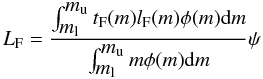 (1)where LF is the total galaxy luminosity, ψ is the SFR, lF(m) is the luminosity of a single star of mass m, tF is the characteristic timescale over which a star of mass m emits radiation in the wavelength band F and φ(m) the IMF. The limits of integration extend over the range of masses of the stars which are expected to emit radiation in the band F. The IMF generally is parametrized as a power law:
 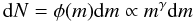 (2)where dN is the number of single stars in the mass range m, m + dm. We adopted a Salpeter IMF defined in the mass range 0.1–100 M⊙ with γ = −2.35 (Salpeter 1955).
The constant of proportionality between SFR and luminosity can be derived by assuming an IMF and a stellar evolution model which provides lifetimes of stars as a function of their masses. The emission from longer lived stars that encodes part or all of the past galaxy SFH dominates in many wavelength bands and only the UV stellar continuum, the emission of optical nebular recombination and forbidden lines (in particular Hα and [OII]) and far infrared (FIR) emission can be used as probes of the young massive star population. Observations made at these wavelengths sample different aspects of the SF activity and are sensitive to different times scales over which SFR is averaged, i.e. the time interval over which radiation is emitted by a massive star in the wavelength band of interest (the continuous SF approximation, Kennicutt 1998).
UV luminosity directly probes the bulk of the emission from young massive stars with a timescale of order of 100 Myr but it is affected by contamination from evolved stars (i.e., the “UV upturn” O’Connell 1999 and references therein) and it is highly sensitive to dust extinction.
However, there is an indirect way to utilise the UV emission as a SF tracer: the UV photons emitted by hot, short-lived stars ionize the surrounding gas to form an HII region, where recombination produces spectral emission lines so we can assume that the massive SF is traced by the ionized gas. The UV continuum and Hα luminosity probe different mass ranges of the massive stellar population: the early and mid B-type stars (5–15 M⊙) can produce much of a galaxy UV continuum, but contribute little to the photo-ionisation of HII regions (Kennicutt 1998). Moreover, the massive stars that can produce measurable amounts of ionising photons (stars with M > 10 M⊙) have considerably shorter lifetimes (about 10 Myr) than massive stars that produce the UV continuum. Of the Balmer lines, Hα is the most directly proportional to the ionising UV stellar spectra, because the weaker lines are much more affected by the equivalent absorption lines produced in stellar atmospheres. This SFR indicator is sensitive to the high end of the IMF, much more than the UV continuum, to dust extinction and to the possible leakage of ionising photons. Moreover, it is also susceptible to the stochastic formation of high mass stars and may not reliably measure the SFR when the activity is low (Lee et al. 2009).
FIR luminosity is a SFR tracer complementary to the UV and optical ones if we assume that much of the stellar light from new-born stars is absorbed, reprocessed by dust (since the cross section of the dust peaks in UV) and emerges in the FIR wavelength region. The efficacy of this SFR diagnostic depends on the fraction of obscured SF and on the optical depth of the dust in star forming regions. The timescale for FIR emission is set by the time it takes massive stars to remove their surrounding material by radiation pressure, expansion of giant HII regions or SN explosions (about 2 Myr). However, this SFR indicator is affected by the contribution to dust heating by older stars and AGNs. Although the FIR luminosity can provide a reliable measure of the SFR only in the most obscured circumnuclear starburst, the combination of the dust-attenuated fluxes in the UV and Hα with measurements of the dust emission in the FIR in the same galaxy sample can provide consistent extinction-corrected SFRs (Kennicutt et al. 2009).
An alternative and complementary approach to trace the SFR is based on the direct observation of the numbers of CC SNe occurring in a sample of galaxies or in a given volume. The CC SN rate (RCC) is given, following the formalism by Blanc & Greggio (2008), by: 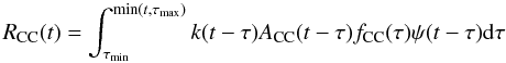 (3)where t is the time elapsed since the beginning of SF in the galaxy under analysis, ψ is the SFR, k(t − τ) is the number of stars per unit mass of the stellar generation born at epoch (t − τ), ACC(t − τ) is the number fraction of stars from this stellar generation that end up as CC SNe, fCC is the distribution function of the time intervals between the formation of the progenitor and the SN explosion (delay times) and τmin and τmax are respectively the minimum and maximum possible delay times. The factor k is given by:
 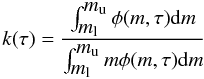 (4)where φ(m,τ) is the IMF and ml–mu is the mass range of the IMF. This factor can change if the IMF evolves with time.
The factor ACC can be expressed by: 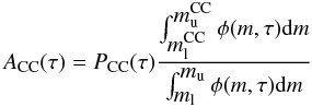 (5)where PCC is the probability that a star with suitable mass (i.e., in the range
  –
– ) to become a CC SN actually does it. This probability depends on SN progenitor models and on stellar evolution assumptions. The factor ACC can vary with galaxy evolution, for example due to the effects of higher metallicities and/or the possible evolution of IMF. We assume that all stars with suitable mass (– ) become CC SNe and PCC(τ) = 1. In the following we also assume that k and ACC do not vary with time, that the delay time for CC SN (~3–20 Myr) is negligible and that the SFR has remained constant over this timescale obtaining a direct relation between CC SN rate and SFR:
 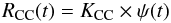 (6)where the scaling factor between CC SN rate and SFR is given by the number fraction of stars per unit mass that produce CC SNe:
 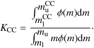 (7)The estimate of the RCC in a galaxy sample needs a systematic SN search with a known surveillance time for each galaxy, i.e. the control time. The control time of a single observation of a given galaxy for a given SN type is defined as the total period of time during which the SN is bright enough to be detected, while observing that galaxy (Zwicky 1938). How long a SN is observable in a given galaxy depends on the SN light curve, host galaxy distance and extinction and on several characteristics of the SN search, such as the limiting magnitude. To determine the total control time of a SN search, we need information on the distribution in time of the single observations of each galaxy and to combine appropriately the control time of each single observation. Another possible approach is to collect as many SNe as possible and the define the galaxy sample from which they emerged (the method of the fiducial sample, e.g. Tammann 1977). In this case the galaxies without SNe enter the sample only according to some selection criteria (e.g. if contained in a given volume).
3. Galaxy sample
Our galaxy sample is based upon the catalogue of the “11 Mpc Hα and Ultraviolet Galaxy Survey” (11 HUGS). 11 HUGS was designed to provide a census of SFR in the Local Volume, to characterise the population of the star forming galaxies and to constrain the temporal behaviour of the SF in low mass galaxies. The design of the 11 HUGS survey, its completeness properties, the observations, the data processing and the characteristics of the galaxy sample are described in Kennicutt et al. (2008) and Lee et al. (2011).
A distance-limit of 11 Mpc was adopted to simultaneously obtain a sample that is statistically significant and nearly complete. Direct stellar distances are available for most galaxies within ~5 Mpc while distances for other galaxies are obtained using the galaxy radial velocity corrected according to the Local Group flow model provided by Karachentsev & Makarov (1996) and the Hubble constant. The galaxy selection consists of two steps: the “primary” sample (261 galaxies) has limits on apparent magnitude (B ≤ 15 mag), Galactic latitude (|b| ≥ 20°) and Third Reference Catalogue of Bright Galaxies (RC3) type (T ≥ 0). The “secondary” sample includes additional 175 galaxies which are either below the magnitude and Galactic latitude limits or lenticular types. The primary sample aims to be as complete as possible in its inclusion of known nearby star-forming galaxies while the overall sample is complete to MB ≤ −15 mag and MHI > 2 × 10⁸ M⊙ for |b| > 20° at the edge of the 11 Mpc volume (Kennicutt et al. 2008). Over the 80% of the sample are dwarf galaxies and low surface brightness systems with SFRs lower than that of the Large Magellanic Cloud.
The Hα observations were obtained with the Bok 2.3 m telescope on the Steward Observatory, the Lennon 1.8 m Vatican Advanced Technology Telescope, the 0.9 m telescope at Cerro Tololo Interamerican Observatory (Kennicutt et al. 2008). The GALEX UV imaging primarily targeted the |b| > 30°, B ≤ 15.5 mag subset of galaxies. The more restrictive latitude limit was imposed to avoid excessive Galactic extinction and fields with bright foreground stars. Deep, single orbit imaging in the far-UV (FUV) and near-UV (NUV) bands was obtained for each galaxy following the strategy of the GALEX Nearby Galaxy Survey (Gil de Paz et al. 2007). Lee et al. (2011) provide full details on GALEX observations and photometry for 390 galaxies: 256 have |b| > 30° and B ≤ 15.5 mag, 120 have lower latitude and fainter magnitude and have been observed by other programmes while 27 galaxies are not included in the 11 HUGS sample. Figure 1 in Lee et al. (2011) shows the resultant GALEX coverage of the overall 11 HUGS sample.
The data from 11 HUGS have further been augmented by Spitzer observations through the composite Local Volume Legacy1 (LVL) program and data from the Two Micron All Sky Survey (2MASS) obtained at 1.25, 1.65, and 2.17 μm. The sample of LVL (258 galaxies) consists of two tiers: the inner one includes 69 early and late type galaxies within 3.5 Mpc that lie outside the Local group for which also Hubble Space Telescope observations exist from the ACS Nearby Galaxy Survey Treasury program and the outer one include a subset of 11 HUGS primary sample with more stringent limits on Galactic latitude. The observational strategy, data processing and photometry measurements are detailed in Dale et al. (2009). Spitzer MIR (IRAC) and FIR (MIPS) data have been obtained for 180 galaxies and the globally integrated 0.15–160 μm spectral energy distribution is obtained from GALEX, 2MASS, IRAS and Spitzer data. Differences in the selection of GALEX and Spitzer samples are due to different adopted distances for some galaxies (see Lee et al. 2011, for more details).
For our analysis we considered three different samples: 383 galaxies (88% of 11 HUGS sample) with measured flux in the Hα (sample A2), 312 galaxies (71%) with both measured flux in the Hα and FUV (sample B) and 167 galaxies (38%) with measured flux in Hα, FUV and TIR (sample C, see Fig. 1).
 |
Fig. 1 The three galaxy samples selected for our analysis with the numbers of galaxies and discovered CC SNe in the last 13 years. |
3.1. Galaxy sample A: Hα luminosities
Integrated Hα luminosity (LHα) are taken from Kennicutt et al. (2008) after applying the following corrections:
-
emission of the [NII](λλ6548,6583) satellite forbidden lines;
-
underlying stellar absorption by subtracting a scaled R band image from the narrow band image;
-
Galactic foreground extinction exploiting the relationship between colour excess and extinction (AHα = 2.5 × E(B − V) mag) by using values based on the maps of Schlegel et al. (1998) and the Cardelli et al. (1989) extinction law with RV = 3.1.
No correction of Hα fluxes for internal extinction was applied in the published catalogue. For about 20% of the sample it was possible to estimate the internal dust extinction via the Balmer decrement, since spectroscopic measurements of Hα/Hβ from the literature are available. We assumed a case B recombination ratio and the Cardelli et al. (1989) extinction law with RV = 3.1 and used the following relation between AHα and Hα/Hβ flux ratio: 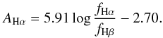 (8)For the galaxies without measurements of the Balmer decrement we adopted an empirical correction scaling with parent galaxy luminosity following the algorithm of Lee et al. (2009):
 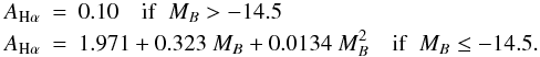 The SFRs have been estimated by adopting the conversion factor by Kennicutt (1998):
  (9)that assumes a Salpeter IMF in the mass range 0.1–100 M⊙, solar metallicity and a constant SFR for at least the past ~10 Myr.
The ratio of Hα flux to the underlying continuum intensity, expressed as an integrated equivalent width (EW(Hα)), has also been measured for 243 galaxies. EW(Hα) is an indicator of the ratio of the current SFR to the total stellar mass (i.e. the specific SFR) that is closely related to the so called stellar birth rate parameter, defined as the ratio of the current SFR to the past averaged SFR. The typical EW(Hα) ranges from zero for early type galaxies up to 20–50 Å for late type galaxies and have values as high as 150 Å for some irregular and unusually active galaxies (Lee et al. 2007).
3.2. Galaxy sample B: Hα and FUV luminosities
The procedure used to perform FUV (~1500 Å) and NUV (~2200 Å) photometry and to measure the FUV luminosity (LFUV) is detailed in Lee et al. (2011). To determine the asymptotic magnitudes, the growth curve in each GALEX band is computed while the aperture fluxes are measured within the outermost elliptical annulus where both FUV and NUV surface photometry can be performed. This annulus has been defined as the one beyond which either the flux error becomes larger than 0.8 mag or where the intensity falls below that of the sky background in both FUV and NUV bands. The fluxes have been corrected for Galactic reddening by using the relationship AFUV = 7.9 × E(B − V), adopting E(B − V) values based on the maps of Schlegel et al. (1998) and the Cardelli et al. (1989) extinction law with RV = 3.1. When TIR data are available the correction for internal extinction is obtained by using the mapping between AFUV and the total infrared to UV (TIR/FUV) flux ratio given by Buat et al. (2005):  (10)where x = log (TIR/FUV). Lee et al. (2009) compared the Hα and FUV attenuation finding a good correlation with a slope AFUV/AHα = 1.8 that is the expected value for the Calzetti obscuration curve and differential extinction law (Calzetti 2001). This agreement provides some assurance that the extinction corrections estimated by Lee et al. (2009) are reasonable and generally consistent. When TIR data are not available or when the equation gives a negative correction, the AFUV was obtained scaling the computed AHα by a factor 1.8 (Lee et al. 2009).
The SFRs in the sample B have been estimated by adopting the conversion factors by Kennicutt (1998) that assumes a Salpeter IMF in the mass range 0.1–100 M⊙, solar metallicity and a constant SFR for at least the past ~ 100 Myr:  (11)
(11)
3.3. Galaxy sample C: Hα, FUV and TIR luminosities
In the sample C, in addition to LHα and LFUV, the total IR luminosity (LTIR) is obtained combining Spitzer MIR and FIR fluxes with with 2MASS NIR data (Dale et al. 2009) with the exception of NGC 628, NGC 1058 and NGC 6949 for which data are from C. Hao (private communication). Elliptical apertures were based on capturing all the galaxy emission visible for all infrared images while for a subset of about 40 galaxies, the infrared-based apertures were slightly enlarged to capture extended UV emission. For a given galaxy, in most cases the same aperture was used for extracting all infrared flux densities. 2MASS fluxes have been extracted for the vast majority of the LVL sample using the same apertures and foreground star removals used to determine IRAC and MIPS fluxes (Dale et al. 2009). LTIR has been used to obtain reliable extinction corrected SFRs according to the prescription of Kennicutt et al. (2009):  (12)LTIR could be also used to estimate the total SFR by adopting the conversion factors by Kennicutt (1998) that assumes a Salpeter IMF in the mass range 0.1–100 M⊙, solar metallicity and for continuous bursts of age 10–100 Myr:
  (13)where LTIR refers to the IR luminosity integrated over the full-IR spectrum (8–1000 μm). We have to stress that this relation applies only to starbursts with age less than 108 years, where the approximations applied by Kennicutt (1998) are valid. In more normal star-forming galaxies the relation between LTIR and SFR is more complicated since the IR emission is still dominated by dust heated by the currently star-forming populations but the contribution from evolved stellar populations could be non-negligible (Kennicutt 1998). Moreover if the galaxies are not completely obscured in the UV, part of UV emission emerges from the galaxy leading to an underestimate of SFR based on LTIR (Kennicutt 1998). Estimating the contamination of evolved populations and the fraction of unabsorbed UV photons is a challenge so we did not adopt the SFR based on LTIR in our analysis.
3.4. B and K band luminosities
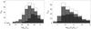 |
Fig. 2 Distribution of LHα (left panel) and LB (right panel), corrected for extinction, in the sample A (empty histogram), sample B (gray histogram) and sample C (black histogram). |
While we now have direct SFR indicators within 11 Mpc and a SN rate for comparison, one would like to put this SN rate into context with previous results within 60–100 Mpc (e.g. Leaman et al. 2011; Cappellaro et al. 1999). Complete and direct SFR measurements (from Hα or FUV) are not available in these more distant galaxy samples hence use of the total B-band and K-band galaxy luminosities is necessary. Trasitionally, SN rates have been normalised to the total luminosity (B-band) or to the total mass.
For each galaxy in the samples A, B and C we determined the B band luminosity (LB) from the observed magnitude and distance adopting MB, ⊙ = +5.48 mag. We correct LB for foreground reddening assuming AB = 1.64 × AHα mag and for internal reddening assuming AB = 0.72 × AHα mag to take into account differential reddening between gas and stars (E(B − V)stars = 0.44 × E(B − V)gas) as discussed in Calzetti (2001). The number of galaxies, the total luminosity in different bands and total SFR for the three samples are summarised in Table 1 while the distributions of LHα, LB for the three samples are illustrated in Fig. 2. Luminosity distributions for samples A and B are quite similar, whereas group C subsamples higher luminosity galaxies.
For each galaxy in the sample C we also determined the K band luminosity (LK) from the observed 2MASS flux (Dale et al. 2009) and distance adopting MK, ⊙ = + 3.28 mag. The galaxy mass can be also estimated in this sample with the method developed by Bell & de Jong (2001) and based on the use of the K luminosity and B − K colour which is an indicator of the mean age of the stellar population in a galaxy: 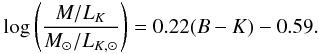 (14)This relation has been obtained by adopting the values from Table 4 in Bell & de Jong (2001) and a Salpeter IMF. Obviously, this method gives a rough estimate of the mass but it can be applied to large samples of galaxies with data available for a limited number of filters. A similar equation has been adopted by Mannucci et al. (2005) and Li et al. (2011a) assuming a “diet” Salpeter to normalise the CC SN rates per unit mass in a larger volume.
Number of galaxies and CC SNe discovered in the last 13 years, the total LHα, LB and SFR for the three samples we have analysed.
4. SN sample
To estimate the CC SN rate we initially identified SNe known to have occurred in the galaxies of the Sample A from the Asiago SN catalogue3 (Barbon et al. 2008) from 1885 to 2010: 38 CC SNe and 10 type Ia SNe (Table A.1). SN 2008iz was discovered in NGC 3034 (M 82) in the radio (Marchili et al. 2010) and its SN nature was confirmed with identification of the expanding ring (Brunthaler et al. 2010). The extinction is extremely high towards this event, and it has not been detected at optical or IR wavelengths, hence we leave it out of our analysis since we are considering only the CC SNe discovered in the optical bands. SN 2008jb, a type II SN, was discovered in archival optical images obtained by the Catalina Real-time Transient Survey and the All-Sky Automated Survey by Prieto et al. (2012). This SN was missed by galaxy-targeted SN surveys and by amateur astronomers mainly because the host galaxy, ESO 302-14 at 9.6 Mpc, is a low-luminosity dwarf galaxy that was not included in the catalogs of galaxies that are surveyed for SNe. We did not consider this SN in our sample but discuss the bias to large star-forming galaxies present in the sample of nearby SNe in the Sect. 7.1.2. Additionally there have been discoveries of 7 Luminous Blue Variables (LBVs) in outburst and three optical transients whose nature is still debated (SN 2008S, NGC 300-2008OT, SN2010da). A possible SN origin from a massive star (>7−8 M⊙) has been proposed for SN 2008S and NGC 300-2008OT by a number of authors (Prieto et al. 2008; Thompson et al. 2009; Botticella et al. 2009; Pumo et al. 2009; Kochanek 2011) but is disputed by others who favour an outbursting massive star event (Smith et al. 2009; Berger et al. 2009; Bond et al. 2009; Humphreys et al. 2011). To be conservative, we will not consider these two transients as genuine CC SNe in our main analysis but we will include them in our discussion of the detectability of CC SNe, since their faint detection magnitudes (with peak magnitudes MR ~ −14 mag) illustrate the depth and completeness of nearby SN searches no matter what their nature. SN 2010da seems to be a LBV-like outburst of a dust enshrouded massive star with bluer colours than those of the progenitors of SN 2008S and NGC 300 OT2008-1. The light curve and spectrum also seem to be different from SN 2008S and NGC 300 OT2008-1 (Khan et al. 2010; Elias-Rosa et al. 2010; Chornock & Berger 2010; Immler et al. 2010; Bond 2010; Prieto et al. 2010)4.
We restrict our comparison between the CC SN rate and the SFR estimates to the last 13 yr (1998–2010), assuming a constant and continuous intensity level of surveillance (i.e., a control time of 13 years). This period is well justified as since 1998 we have witnessed a large increase in the discovery rate of SNe in the Local Universe. This is due to the start of Lick Observatory Supernova Search (LOSS) in 1998 that monitored about 15 000 galaxies with z < 0.05 for 13 years and discovered about 1000 SNe (Leaman et al. 2011; Li et al. 2011a) and the high number of amateurs searching SNe in the nearby galaxies who have been using telescopes of 20–50 cm and modern CCDs for the last ~15 years.
The majority of the CC SNe within 11 Mpc in the last 13 years (Table 2) have been discovered by amateur astronomers (60% of events) with 40% coming from the LOSS professional searches. The distribution of the discovery epoch with respect to the maximum light, of the discovery magnitude and the absolute magnitude at maximum light of our SN sample are illustrated in Fig. 4.
At a typical distance modulus of 31 mag for the most distant galaxies in our sample, the limiting magnitude of ~18–19 mag in the SN searches results in detections down to MR ~ −12 mag for unreddended events. CC SNe which are not heavily extinguished or intrinsically faint stay above 18 mag for about 200 days (Fig. 3). Hence we can be fairly sure that significant numbers have not been missed due to solar conjunction or a lack of searching by the global community. One observation every few months is sufficient to ensure that the normal SN population is well surveyed. Of course, there may be a population of significantly extinguished SNe, or intrinsically faint SNe. For a typical IIP, with MR ~ −16 mag, one might expect the surveys to be sensitive to SN obscured by about 4 mag. Indeed two SNe (2002hh and 2004am) have been discovered by LOSS (Leaman et al. 2011; Li et al. 2011a) which were faint but located in quite nearby galaxies. The expected dust obscuration was confirmed with extinction estimates of AV = 5.2 and 3.7 mag respectively (Pozzo et al. 2006; Smartt et al. 2009). It is not implausible to argue that there are more obscured local events evading detection in the optical bands.
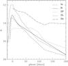 |
Fig. 3 The observed light curves of different unreddened CC SN sub-types at 11 Mpc. The absolute magnitudes in R band at maximum are –19.16 mag for type Ia SNe, –17.92 mag for type Ib SNe, –16.38 mag for type IIP SNe, –17.70 mag for type IIL SNe and –17.14 mag for type IIn SNe. Phases are relative to the maximum epochs. |
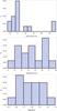 |
Fig. 4 The distribution of the discovery epoch with respect to the maximum light, of the discovery magnitude and absolute magnitude at maximum for our SN sample. The values for each CC SN and sources are reported in Table 2. |
In our CC SN sample four events (SNe 2002ap, 2005cs, 2008ax, 2008bk) were discovered soon after the explosion (within a few days of shock breakout). Five of the events were discovered either before light-curve maximum (SNe 2007gr, 2008S and NGC 300-2008OT), or early in the plateau phase (SNe 2002hh, 2004et). The other four events (SNe 2003gd, 2004am, 2004dj, 2005af) are type IIP SNe discovered during mid-plateau. Early discoveries of SNe 2003gd and 2004dj were missed simply due to the galaxies being in solar conjunction at SN explosion epoch. All of this supports our view that the A, B and C galaxy samples have been systematically surveyed during the last 13 years, and the CC SN rate is at least reliable enough for a meaningful comparison with the SFR estimates now available. It is of course a robust lower limit.
Restricting our CC SN sample to that discovered in the last 13 years has another advantage. All of the SNe are spectroscopically classified and the majority have extensive photometric and spectroscopic coverage of their evolution. We do not subdivide our small sample into different CC SN sub-types since individual bins contain only few objects. Smartt et al. (2009) compiled all SN discoveries in a fixed period (10 years) within a fixed distance (28 Mpc) and estimated the relative frequency of all subtypes (58.7% type IIP, 2.7% type IIL, 3.8% type IIn, 5.4% IIb, 9.8% Ib, 19.6% Ic). In a larger 60 Mpc volume, the LOSS survey (Li et al. 2011a) has estimated: 48.2% type IIP, 6.4% type IIL, 8.8% type IIn, 10.6% IIb, 26% Ibc. Our smaller sample has 60% type IIP SNe, and the other 40% as such it is too small to attempt any further meaningful subdivision, but the overall ratios are similar to the LOSS and 28 Mpc volumes.
SN type, SN magnitude at the discovery epoch and at maximum light, phase (days) between the discovery epoch and the maximum light for the CC SNe discovered within 11 Mpc in the last 13 years, the host galaxy’s name, morphological type, B band absolute magnitude, SFRs (M⊙ yr-1), B − K colour, mass (1010 M⊙), specific SFR (yr-1) and EW(Hα).
The distribution of LB, LK, SFRs, B − K, mass specific SFR and EW(Hα) for the galaxies in the sample C that hosted CC SNe are illustrated in Fig. 5. The host galaxies have highest SFRs, luminosities and masses, while their distribution in B − K, sSFR and EW(Hα) is more shallow.
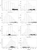 |
Fig. 5 The distribution of the LB, LK (in LB, ⊙ and LK, ⊙ unit), SFRs, B − K, mass, specific SFR and EW(Hα) for the galaxies that hosted SNe (full histogram) and all the galaxies (empty histogram) in the sample C. |
5. Comparison of SFR indicators
The number of SN discoveries within the 11 Mpc volume makes for an interesting comparison between the SFRs obtained from the observed CC SN rate and those based on multi-wavelength flux measurements. Each provides an independent measurement which suffers from different uncertainties and biases. The CC SN rate is likely biased towards the brighter SNe and maybe systematically misses a population of SN explosions (due to either modest intrinsic brightness or large extinction) so it gives a lower limit for the current SFR.
Dust extinction is probably the largest source of systematic uncertainty in the direct measurements of SFRs. Different SFR tracers are affected by extinction to different extents: typical dust attenuation is of order 0–2 mag in Hα and 0–4 mag in UV continuum (Kennicutt et al. 2009). The resulting systematic error in the overall SFR measurements is generally removed by applying a statistical correction for dust extinction (Kennicutt 1983; Calzetti et al. 1994, 2000) or by combining observations in UV and Hα with those in the IR wavelength range (Kennicutt et al. 2009).
In order to estimate the SFR from CC SN rate measurements we have to assume the mass range of CC SN progenitors and to correct the rates for the fraction of the extinguished CC SNe that are missed in optical searches. The lower mass limit for CC SN progenitors from direct detections of progenitor stars in high-resolution images has arrived at a best estimate of  M⊙ (Smartt et al. 2009), which is in reasonable agreement with the most massive white dwarf progenitors (Williams & Bolte 2007; Williams et al. 2009). This has led Smartt (2009) to suggest that the current best estimate from these two methods is 8 ± 1 M⊙. If we assume this value of 8 M⊙ the observed CC SN rates in the galaxy samples A, B and C imply SFRs are plotted in Fig. 6. The observed CC SN rate is of course only a robust lower limit since we have not applied any correction for undetected SNe. The SFR from CC SNe is higher by a factor two compared with those in Sample A and C based on LHα while there is good agreement with SFR based on LFUV that suggests we are not missing a large number of CC SNe within 11 Mpc due to dust extinction, intrinsically faint magnitudes, or over-estimating the control time.
The main source of the difference between the corrected SFRs based on LFUV and LHα is due likely to the attenuation corrections. A few of the galaxies with the highest SFRs tend to show especially large discrepancies between LFUV and LHα derived SFRs, and we suspect that some of these may arise from spurious causes such as extremely heavy extinction in edge-on systems (e.g., M 82), very large foreground Galactic extinction (e.g., NGC 6946), or poorly measured Hα fluxes (e.g., NGC 6744). These galaxies carry disproportionate weight in the total SFRs for the samples, but even taking them into account the LFUV based SFRs remain systematically larger.
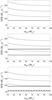 |
Fig. 6 From the top to the bottom: the SFR expected from the CC SN rate in the sample A, B and C (thin lines) as a function of the upper mass limit for CC SN progenitors. We adopted a lower mass for CC SN progenitors of 8 M⊙. We plot the central value and 1σ confidence limits. The short dashed line indicates the value of SFR based on LHα (in all panels: sample A, B and C), the short dashed line the SFR based on LFUV (middle and bottom panels: samples B and C) and long dashed line the SFR based on LHα + LTIR (bottom panel: sample C). |
A small part of the offset comes from the adoption of the Buat et al. (2005) formula for estimating LFUV extinction corrections. Kennicutt et al. (2009) compared attenuations derived from that method with those from Hα +TIR and Hα +24 μm schemes, and found that the former are systematically larger, by about 0.1–0.2 mag. There is also a more important systematic offset (30–40%) in TIR luminosity between MIPS, which was used for nearly all of our sample, and IRAS, which was used to calibrate the Buat et al. (2005) relation (for more details see Figs. 1–2 of Kennicutt et al. 2009). This difference is only important for galaxies with cold IRAS colours (where basically the IRAS wavelength coverage is not sufficient to integrate the IR emission reliably). Unfortunately that colour regime applies to most of our galaxy sample.
The comparison between CC SN rate and SFR based on other diagnostics has also been done at larger volumes (Dahlen et al. 2004; Botticella et al. 2008; Bazin et al. 2009; Horiuchi et al. 2011) and points out a discrepancy in the opposite direction with respect to the local universe since the observed CC SN rate is lower than the predicted one from SFR measurements. It is interesting to note that this discrepancy (about a factor two) is constant in a large range of redshift (Botticella et al. 2008; Horiuchi et al. 2011). Dale et al. (2010) estimated the SFR density in four different redshift bins (z ~ 0.16,0.24,0.32,0.40) exploiting the data from the Wyoming Survey for Hα (WySH). LHα has been corrected for dust extinction by using the luminosity dependent prescription of Hopkins et al. (2001) and the volume averaged SFR has been estimated by integrating under the fitted Schechter function and adopting the Kennicutt (1998) conversion factor. The evolution of the cosmic SFR density suggested by these measurements are well fitted by a power law ρSFR = ρSFR(0)(1 + z)4.5 ± 0.7, while if we consider also the other results of recent emission line surveys for the SFR density over 0 ≤ z ≤ 1.5 the evolution is given by ρSFR = ρSFR(0)(1 + z)3.4 ± 0.4 (Hopkins & Beacom 2006; Horiuchi et al. 2009; Dale et al. 2010). The evolution with redshift of the volumetric CC SN rate can be fitted with a power law (1 + z)3.6 (Botticella et al. 2008; Bazin et al. 2009) so the CC SN rate evolution seems to be consistent with that of SFR in a wide range of redshift but there is a problem in the normalisation (Hopkins & Beacom 2006; Botticella et al. 2008; Beacom 2010; Horiuchi et al. 2011). We also emphasise that the prediction of the stellar mass density based on the integrated SFH also exceeds the observed value at the present epoch by a factor of two and remains systematically higher with cosmic time evolution5 (Wilkins et al. 2008). Horiuchi et al. (2011) have analysed the normalization discrepancy between predicted and measured CC SN rates in the Local Volume (d ≤ 100 Mpc) exploring whether the cosmic CC SN rate predicted from the cosmic SFR is too large, or whether the measurements underestimate the true cosmic CC SN rate, or a combination of both. They suggested three main possible outcomes: half of stars6 with masses 8–40 M⊙ are producing dim CC SNe, either due to dust obscuration or being intrinsically weak, and the fraction of dim CC SNe could explain the normalization discrepancy; there is a high fraction of optically dark CC SNe while the dim CC SN fraction is only slightly higher than the most recent SN luminosity function of LOSS (Li et al. 2011b); the normalization discrepancy could be explained by systematic changes in our understanding of SF or CC SN formation. The main concern in the CC SN rate measurements at higher redshift is the dust extinction correction since the level of dust obscuration is expected to be higher. Mannucci et al. (2007) derived that the fraction of missing CC SNe is only ~15% at intermediate redshift, far too small to fill the gap between observed and predicted rates. To obtain an acceptable agreement between the measurements of CC SN rate and the predictions with the SFH as compute in Hopkins & Beacom (2006) requires an average E(B − V) = 0.3 mag at z = 0.3 and E(B − V) = 0.5 mag at z = 0.7 (Dahlen et al. 2004; Hopkins & Beacom 2006) or the high extinction scenario adopted in Botticella et al. (2008). These values are quite extreme and require an extremely high dust content in galaxies which is not favoured by present measurements or inferred from the luminosity-dependent obscuration corrections for UV and Hα data at similar redshifts. Moreover, we have to stress that the extinction in a region nearby a CC SN can be higher than the average attenuation in the host galaxy.
6. Estimate of the CC SN progenitor mass range
The mass range of CC SN progenitors can be observationally constrained by comparing the birth rate of stars and the rate of CC SNe in the same galaxy sample assuming a distribution of the masses with which stars are born. The simplest Poisson model formulation is to compare the total observed number of CC SNe(NCC) to the expected number (⟨NCC⟩): 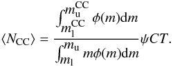 (15)The posteriori density function (PDF) can then be expressed as the Poisson probability with a prior accounting for the total observed SFR in the galaxy sample:
 ![Mathematical equation: \begin{equation} {\cal{L}} \propto \NCCExp^{\ncc} \exp \left[ -\NCCExp \right] \times \exp \left[ -\frac{(\psi-\psi_\mathrm{obs})^2}{2 \delta \psi^2 } \right]\cdot \lab{like2} \end{equation}](/articles/aa/full_html/2012/01/aa17343-11/aa17343-11-eq173.png) (16)As estimators for the central value and scale, we used the mean and the standard deviation of PDF. We considered flat, rather than informative priors for the initial masses, i.e.,
(16)As estimators for the central value and scale, we used the mean and the standard deviation of PDF. We considered flat, rather than informative priors for the initial masses, i.e.,  and
and 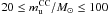 . A different approach would have been to consider each galaxy as the source of a random process and to obtain the joint probability function as a combination of Poisson distributions. We found no statistical improvement using this variant, so we prefer to illustrate the simpler approach.
The SNe discovered by the old local SN surveys (Asiago, Crimea, Evans, OCA and Calan Tololo searches) and exploited by Cappellaro et al. (1999) to obtain SN rate measurements at z < 0.01 have been collected from 1960 to 1997 so it is possible to merge this SN sample with that of SNe discovered in the last 13 years. We cross matched our galaxy samples with the galaxy sample from Cappellaro et al. (1999) (7773 galaxies) and found 201 common galaxies with the sample A and 8 CC SNe, 3 type Ia and 2 unclassified SNe7 discovered in these galaxies, 167 common galaxies with the sample B and 8 CC SNe, 112 galaxies in common with the sample C and 7 CC SNe. The unclassified SNe have been redistributed among the three SN types according to the observed distribution: 100% type Ia in E–S0, 35% type Ia, 15% type Ib and 50% type II in spirals. By taking into account SNe discovered from 1960 we increase the number of CC SNe from 14 to 23.3 in the sample A, from 13 to 21.3 in the sample B and from 12 to 19.7 in the sample C. Obviously to use both SN samples we have to properly combine, for the galaxies in common, the control times of the past SN surveys and the assumed control time in the last 13 years.
In our analysis we considered for each galaxy sample two SN counts: the SNe discovered from 1998 to 2010 (this gives  ) and the SNe discovered from 1960 to 2010 (this gives
  ). When considering the extended period (1960–2010) we should add a third variable to the likelihood function to account for the number of actual CC SNe which are within the unclassified group and we should marginalise over. However, we verified that the simpler approach gave the same results i.e. we considered an effective number of CC SNe in the Poissonian likelihood, as given by the mean number of CC SNe expected in an unclassified sample (taking the local estimates for spiral galaxies). Results for the different galaxy and SN counts are reported in Table 3 and are statistically consistent.
Estimated minimum mass in different galaxy samples and for different SN samples.
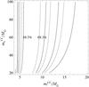 |
Fig. 7 Probability density function of |

The likelihood in the  plane after marginalization over ψ is plotted in Fig. 7 for the sample B. The contours in the figure correspond to the 68.3%, 95.4% and 99.7% confidence limits for two parameters, obtained as ℒ/ℒmax = exp − 2.30/2, exp − 6.17/2 and exp − 11.8/2, respectively. These values, which make sense only in a frequentist statistical analysis, are plotted only to illustrate parameter degeneracies. As expected contours are very elongated and no significant constraint can be put on the upper limit mass of CC SN progenitors.
The PDF for  is plotted in Fig. 8. We note a sharp decline at low masses, whereas the tail at larger values is quite shallow.
 |
Fig. 8 Posterior probability density function for |
An independent measurement of the CC SN rate in a larger galaxy sample, i.e., the estimate by Cappellaro et al. (1999) at z < 0.01, can be used as a statistical prior to further constrain the lower mass of CC SN progenitors when we take into account only the CC SNe discovered in the last 13 years (Table 3, column  ). In general adding such a prior brings about two effects (Fig. 8): the peak of the PDF shifts towards higher values of and the tail for large masses is reduced. The overall effect on the final estimate is that the mean is nearly unchanged whereas the standard deviation is lowered.
The results in the three galaxy samples are in agreement within the uncertainties however the mean value obtained in the sample B is higher than those in the other two samples. In fact in the sample B we have a total SFR a factor of 1.4 higher than that in the sample A and a very similar number of SNe. If we consider LHα based SFR in the sample B with a dust extinction correction via Balmer decrement and a control time of 13 years and NCC = 13 we still obtained  M⊙.
M⊙.
7. Systematic errors
The method to estimate the mass cutoff for CC SN progenitors described in the previous section needs a well defined galaxy sample with accurately measured SFRs and a systematic SN search for which all information required to calculate the CC SN rate is available. There are several possible sources of error in our analysis: a systematic underestimate of the CC SN rate, systematic errors in the SFR estimate, systematic errors in the adopted IMF and distance scale. The effect of such errors on the derived minimum mass for the CC SN progenitors will be discussed in turn.
7.1. SN rate
There are two effects that would depress the absolute CC SN rates: the underestimate of the SN number and the overestimate of the total CT of the galaxy sample. It is difficult to accuratley determine the degree of uncertainty due to both these effects since the surveys that discover local SNe are a combination of professional and amateurs with complicated and unquantified selection functions. However we can estimate both uncertainties.
7.1.1. SN sample
Estimated minimum mass of CC SN progenitors in different galaxy samples derived considering a control time of 13 years and different assumptions about the number of CC SNe discovered in the last 13 years, the maximum mass for progenitors of CC SNe with optical signature, the IMF and the distance scale.
The incompleteness of our SN sample depends both on the extinction suffered by CC SNe and on the fraction of intrinsically faint CC SNe that are missed by local SN surveys.
Dust extinction is the largest source of systematic uncertainty in measurements of CC SN rates. The fraction of CC SNe (about 5%) that can be missed in the optical searches in the local universe derived by Mannucci et al. (2007) is much smaller than the uncertainties in the measured rates since SN statistics is still confined to small numbers in the local universe.
How many nearby SNe are missed owing to their intrinsically faint luminosities is still uncertain. Two intrinsically faint transients which have dust-embedded progenitors (SN 2008S, NGC 300-OT2008) have been recently discovered and two plausible scenarios have been suggested to explain the characteristics of their progenitors and explosions: outbursts of massive stars (Smith et al. 2009; Berger et al. 2009; Bond et al. 2009) or EC SNe in super-AGB stars (Prieto et al. 2008; Thompson et al. 2009; Botticella et al. 2009; Pumo et al. 2009). Thompson et al. (2009) estimated that the transients like SN 2008S are the 9% of all optical transients discovered within 10 Mpc when averaged over the last 10 yr and estimated a correction for incompleteness is close to a factor 2. Including the two dubious SNe (SN 2008S and NGC 300-OT2008), we have 16, 15 and 14 CC SNe in the sample A, B and C respectively. This has the expected effect of pushing the value to lower masses. In this case less massive progenitor are favoured, but the change is not very significant (about 10%, Table 4 and Fig. 7).
Finally some massive stars are expected to produce weaker explosion with a black hole formed by fallback (25–40 M⊙) or collapse into a black hole directly (>40 M⊙) without any optical signature (failed SNe), contributing to the UV or Hα luminosity of the galaxies but not the observed CC SN rate. The predicted mass range of failed SNe depends on rotation and metallicity (Heger et al. 2003; Limongi & Chieffi 2003). The lower mass cutoff for CC SN progenitors is not strongly dependent on the choice of the maximum mass since the steep power law nature of the IMF guarantees that a majority of the progenitors have masses within a factor 2 of the lower limit mass regardless of whether the mass spectrum extends to very high mass. If we conservatively restrict the upper mass limit of detectable CC SN progenitors to mup < 30 M⊙ and considering the 14 CC SNe discovered in the last 13 years this reduces the minimum mass estimate by about 5% and 11% in the sample A and B respectively (Table 4). In other words, the value of is not particularly sensitive to the highest mass that can produce a CCSNe.
7.1.2. Control time
Some galaxies in our sample might have been monitored only for a short period or might have not been monitored at all. For example SN 1996cr8 was missed at a distance of 3.8 Mpc (Bauer et al. 2008; Dwarkadas et al. 2010).
To investigate the influence of different control times of different regions of the sky the galaxy sample has been divided in three different groups located in regions of celestial sphere with similar area. We considered the fraction of the galaxies, the fraction of B band luminosity and the fraction of discovered SNe for each group (Table 5). The fraction of discovered SNe is very similar to the fraction of galaxies and LB so we can exclude that the SN search coverage in the northern hemisphere is significantly better than in the southern one (Fig. 9).
Fraction of galaxies, B band luminosity and discovered SNe in three different regions of the sky.
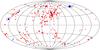 |
Fig. 9 The sky distribution of the galaxies in our sample A (red points). Blue points represent the galaxies that hosted CC SNe. The dimension of points is proportional to the CC SN number. |
Different types of galaxies and SNe seem to be scattered randomly over the sample area so the incompleteness factor depends very little on the position of the galaxy within the sample.
A selection effect may be due to galaxy luminosity since the galaxies targeted by either local SN surveys or amateurs are predominantly large, luminous and metal-rich. It is very difficult to quantify the bias against faint dwarf galaxies. However, the number of missed CC SNe in dwarf galaxies in the last 13 years should be not high due to the their low SFRs. Only two out of 14 SNe in our sample were discovered in dwarf galaxies. SN 2008jb, which exploded in the southern dwarf irregular galaxy ESO 302?14 and it is not included in our sample, was recently discovered in archival optical images obtained by the Catalina Real-time Transient Survey and the All-Sky Automated Survey by Prieto et al. (2012). The statistical error due to the SNe discovered in dwarf galaxies (~1–2) is negligible with respect to the Poissonian error of the overall SN sample (~3–4) so this does not affect our results.
Finally we compared the SN discovery rate within 11 Mpc, 60 Mpc and in the whole Universe from 1997 to 2009 (Fig. 10) to search for any possible fluctuation in the discovery rate within 11 Mpc. The SN discovery rate within 11 Mpc is almost constant during the last 13 years.
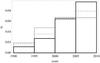 |
Fig. 10 The discovery rate of CC SNe from 1990 to 2009. The thick, dashed and thin lines are for CC SNe discovered in the whole Universe, within 60 Mpc and within 11 Mpc, respectively. |
Hence the SN sample and CT uncertainties imply that any corrections in the future would decrease our estimate of the lower mass limit to produce a CC SN. It is unlikely that any of these uncertainties could work in the opposite direction.
7.2. SFR
The systematic uncertainty in the determination of the SFR is comparable with the statistical fluctuation in the Poissonian distribution. In sample C, we found a 30% difference between the lower mass limit calculated with SFRs from LHα and LFUV. A similar result is obtained by comparing the low mass estimates in the sample A and B. The results obtained by adopting SFRs based on LHα but with different dust extinction corrections, derived from the Balmer decrement and TIR luminosity, are in excellent agreement. This is not be surprising since the TIR+Hα recipe was partially calibrated using the LHα for galaxies that had Balmer decrements available.
7.3. IMF
Subsequent studies to the early measurement of IMF by Salpeter (1955) found that there is a clear flattening in IMF slope around 0.5 M⊙ and a further flattening near the sub-stellar mass limit so the IMF at the low mass end is well represented by either a series of broken power laws (Kroupa 2001) or with a log-normal function (Chabrier 2003). While there is still some debate regarding the peak and the turnover in the IMF, the high mass end is typically well described by the Salpeter slope for a wide variety of environmental conditions (Massey 2003; Elmegreen 2009). Uncertainties of the IMF slope for massive stars are due to uncertainties in theoretical stellar models but variation around the Salpeter value is limited to approximately ± 0.5. If we adopt in our analysis a Kroupa (2001) IMF with γ0 = 0.3 for 0.01 ≤ m/M⊙ < 0.08, γ1 = 1.3 for 0.08 ≤ m/M⊙ < 0.5 and γ2 = 2.3 for 0.5 ≤ m/M⊙ ≤ 100 and the corresponding scale factors between luminosities and SFR we obtain very similar results for the lower mass of CC SN progenitors (Table 4).
However, recent researches indicate that the supposedly universal IMF within young star clusters does not necessarily yield the same average IMF over a whole galaxy, refered to as the integrated galaxial IMF (IGIMF). The IGIMF could be deficient in high mass stars compared to the IMF since the maximum stellar mass in a cluster seems to be limited by the embedded total cluster mass (Kroupa & Weidner 2003; Weidner & Kroupa 2005). A further complication arises from the possibility that the maximum embedded star cluster mass steepens with decreasing SFR so it is constrained by the current SFR (Pflamm-Altenburg et al. 2007, 2009). The combination of these two effects gives a IGIMF which is steeper in the massive range than the Salpeter IMF and is dependent on the SFH of the galaxy. If the IMF varies between galaxies there could be substantial variations in the conversion of Hα or UV flux to SFR (Hoversten & Glazebrook 2008), the number of CC SNe per stellar generation could be suppressed relative to that expected for a Salpeter IMF and dwarf galaxies could have a suppressed number of CC SNe per formed stellar generation relative to massive galaxies. Given the uncertainties, more extensive analysis of the issue is beyond the scope of this paper.
7.4. Binarity
The study of young stellar populations revealed that most stars are in binary or higher order multiple systems and that the binarity fraction among stars is a function of mass (Zinnecker & Yorke 2007). In particular, the observed fraction of O stars in massive multiple systems lies between at least 20 and 80% (Weidner et al. 2009, and reference therein). For typical models of binary statistics, 50–70% of CC SN progenitors are members of a binary system at the time of the explosion (Kochanek 2009).
The Salpeter IMF is not corrected for binarity. A limited number of studies have addressed how the large proportion of binaries affect IMF measurements since multiple system that are not resolved into individual stellar companions hide the less luminous members (Kroupa 2002; Maíz Apellániz 2008; Weidner et al. 2009). Kroupa (2002) suggested that the slope value of IMF may be artificially large at high masses (γ = 2.7) due to the effect of unresolved binaries. Weidner et al. (2009) studied the influence on the IMF of large quantities of unresolved multiple massive stars and found that even under extreme circumstances (100% binaries or higher order multiples), the difference between the power-law index of the mass function of all stars and the observed IMF is small (~0.1). They concluded that if the observed IMF has the Salpeter index γ = 2.35, then the true stellar IMF has an index not flatter than γ = 2.25.
However, the binarity affects also other parameters involved in our calculations. The presence in a binary system can increase the mass loss and mass transfer and dramatically affect the stellar evolution. This has two important effects: a different scaling factor of SFR tracers predicting the correct ionising flux and a different structure of the core of a massive star at the time of core collapse. We did not consider these effects in our analysis.
7.5. Distance scale
The typical distance uncertainties in our galaxy sample are of 5–6% for a galaxy with direct stellar measurements and 15% for a galaxies with distances obtained from secondary indicator or with flow based distances (Kennicutt et al. 2008). If the distances were systematically underestimated by 10% we would find a difference of ~10% in the mass cutoff for CC SN progenitors (Table 4).
In summary the uncertainties in CC SN rate act to decrease the lower mass limit of CC SN progenitors, the uncertainties in dust obscuration correction for SFR estimates can raise it, while the choice of the IMF from Kroupa (2001) systematically increases the lower mass limit. Individually these are each less than a 10% effect.
8. Comparison with other observational estimates
The first time that the linear correlation between LHα and CC SN rate was exploited to determine a lower mass limit for CC SN progenitors was by Kennicutt (1984). This study used a sample of 80 nearby Sc-SBc galaxies and combined them with an estimate of the CC SN rate (1.4 ± 0.2 SNu) in face-on Sc-SBc from Tammann (1982) assuming an “extended” Miller-Scalo IMF (γ = 2.5 between 1–100 M⊙) and H0 = 50 km s-1 Mpc-1. Although Kennicutt (1984) used one of the earliest estimates of the CC SN rate based on few events and a different IMF his result, scaled to H0 = 75 km s-1 Mpc-1, of  M⊙ is consistent with our estimate in the sample A.
Blanc & Greggio (2008) compared the redshift evolution of the CC SN rate with a parametric form of the SFH found a minimum progenitor mass greater than 10 M⊙. Although they admit that incompleteness in the observed CC SN rate would imply a lower mass. Maoz et al. (2011) used 119 SNe from the the LOSS survey and compared this rate to the SFHs of individual galaxies. They derived the SFHs for 3505 galaxies with SDSS spectra by using the VESPA code and assuming a dust model. The CC SN rate of 0.010 ± 0.002 SNe per M⊙ is in agreement with expectations if all stars more massive than 8 M⊙ give CC SNe. Maoz et al. (2011) also suggest that their SN rate estimates argue against a significant fraction of massive stars collapsing without producing a visible and detectable SN. In other words, that the upper mass limit must be quite high. However as shown in Fig. 6 the upper mass limit for CC SNe is quite unconstrianed from SN rate measurements above 20 M⊙. The CC SN rates themselves can’t quanitatively constrain the upper mass limit within the ~20–150 M⊙ range (simply due to the steep power law nature of the IMF).
The direct detection of progenitor stars in pre-discovery images has provided identifications, mass estimates and mass limits for over 20 CC SNe (see Smartt 2009 for a review). Smartt et al. (2009) carried out a detailed and homogeneous analysis of all II-P SNe progenitor searches within 28 Mpc. A maximum-likelihood analysis gives the best fitting minimum and maximum masses for the SNe IIP progenitors,  M⊙ and 16.5 ± 1.5 M⊙ respectively, assuming a Salpeter IMF. The minimum mass is consistent with our estimate within the errors. This lower mass limit is consistent with other studies of type II progenitor stars (Maund et al. 2005; Li et al. 2006; Mattila et al. 2008; Van Dyk et al. 2010; Fraser et al. 2011). However some estimates of the hydrodynamic mass of the ejected enevlopes of IIP SNe give systematically higher results, e.g., 9–12 M⊙ in Zampieri (2007) and 15–30 M⊙ in Utrobin & Chugai (2009). While there is no systematic study of a large enough sample to produce an estimate of the lower mass limit, the discrepancy should be taken seriously in attempts to determine masses from both methods.
The mass dividing CC SN progenitors from WD progenitors is theoretically expected to lie in the mass range 7–11 M⊙ depending on metallicity and the degree of overshooting (Siess 2007). Observations of most massive WD progenitor in young star clusters provide a lower limit on the value of this mass (Koester & Reimers 1996). Williams & Bolte (2007) and Williams et al. (2009) studied the WD populations in the open clusters of NGC 6633, NGC 7063 and NGC 2168 and found a lower limit on the maximum mass of WD progenitors between 6.3–7.1 M⊙. This result is also consistent with our estimates of the minimum mass for CC SN progenitors.
The minimum mass for CC SN progenitors is an important factor in the study of Keane & Kramer (2008), to estimate the birth rate of the Galactic neutron star population. They took an estimate of the Milky Way CC SN rate of 1.9 ± 0.9 per century from the measurements of the Galactic 1.809 MeV emission line from the radioactive decay of 26Al (Diehl et al. 2006). Alternatively, they assumed a lower mass limit of 11 M⊙, and a Milky Way SFR of 4 M⊙ yr-1 to arrive at the same CC SN rate (1.9 ± 0.9 per century). This appears to be significantly lower than the observed population of pulsars, rotating radio transients, X-Ray dim isolated neutron stars and magnetars, which imply a neutron star birth rate of 10.8 per century. Our results in this paper and those on the direct progenitor detections and WD progenitor limits, argue for lower values of . It appears that a value of 10–12 M⊙ for is disfavoured by the combination of all these studies. A value of 7 M⊙ would not be inconsistent within the three independent estimates and that would increase the Milky Way SN rate to 4.4 ± 2. This is still below the high neutron star birth rate estimate, but just within the 1σ error.
9. Conclusions
The massive star birth and death rates are tightly correlated due to their short lifetime. We can exploit the CC SN rate as a diagnostic of the current SFR by assuming an IMF and a mass range of the CC SN progenitor. Conversely we can obtain a significant constrain on the CC SN progenitor mass range by assuming a SFR inferred through the galaxy luminosity.
Only the estimate of CC SN rate in a well defined galaxy sample can provide a direct link between SN rates and different stellar populations. Complete and volume-limited SN and galaxy samples are crucial to perform a statistically meaningful analysis and the advent of large sets of multi-wavelength observations of nearby galaxies from the 11 HUGS and LVL programmes provide us, for the first time, the opportunity to compare SFRs based on CC SN rate and more established tracers in the same galaxy sample. The data are complete enough that we can take into account the different uncertainties and biases that affect these SFR diagnostics. Assuming a lower mass limit cut-off of 8 M⊙ for CC SN progenitors and a Salpeter IMF for massive stars, we find that the SFR based on LHα can not reproduce the observed CC SN rate while there is a good agreement with SFR based on LFUV in our galaxy sample. The multi-wavelength data allow LHα to be corrected by adopting different dust extinction corrections, from either the Balmer decrement or by combining TIR and Hα luminosity. Even with this correction, our analysis suggests that LHα may under-estimate the total SFR in our galaxy samples, by nearly a factor of two.
A future prospective of this analysis is to study the connection between SFR tracers and CC SN rate on a galaxy-by-galaxy basis and to compare the spatial distribution of CC SNe with that of the SFR in spiral arms. Multi wavelength data also will also allow us to better constrain the dust effect and in principle to discriminate the fraction of missed SNe due to the dust extinction and failed SNe.
Conversely, we assumed that the SFRs based on Hα and FUV luminosity are reliable and obtained an observational constraint on the mass range of CC SN progenitors by comparing the expected number of CC SNe from SFR measurements with the observed number in our galaxy samples. Our analysis suggests that the minimum mass to produce a CC SN is 8 ± 1 M⊙ or 6 ± 1 M⊙ if we consider FUV and Hα based SFR, respectively. The first result is in excellent agreement with that obtained by analysing a sample of nearby SNe with detected progenitor stars (Smartt et al. 2009). Obviously, assuming SFRs inferred through LHα a larger mass range is required to fit the expected and observed numbers of CC SNe.
Recent comparisons between the SFR and CC SN rate at redshifts between z = 0−1 have suggested a discrepancy between the two, with the numbers of CC SNe detected being too low by a factor of two (Botticella et al. 2008; Horiuchi et al. 2011). The very Local Volume of 11 Mpc which we study here does not show that discrepancy. This is likely due to the faint events (both intrinsically faint, and obscured) being missed outside the 11 Mpc volume and would suggest that even in the nearby Universe, SN surveys are incomplete. The uncertainties in our calculations (Poissonian and systematic) are not low enough to rule out that some massive stars collapse to black holes and produce optically dark SNe.
Few galaxies edge-on (with Hα extinction estimates under-estimated), or with very high Galactic foreground extinction (with uncertain corrections especially in the FUV) have been removed from our galaxy samples (UGC 2847, NGC 5055, NGC 5195, NGC 6744).
There are 10 further events that have not been spectroscopically classified but are likely SNe of some sort, and an additional faint transient in NGC 4656 discovered in 2005 of unknown origin (Rich et al. 2005; Elias-Rosa et al. 2005) that we leave it out of our analysis. However none of these are in our 11 Mpc and 13 yr SN sample.
An IMF with a high-mass slope shallower (γ = 2.15) than the Salpeter slope can reconcile the observed stellar mass density with the cosmic SFH, but only at low redshifts (Wilkins et al. 2008).
This is possible if some SN impostors, as SN 2008S, are true CC SNe.
(1969L, 1969P, 1973R, 1980K, 1982F, 1983N, 1984R, 1985F, 1986G, 1987A, 1989B, 1993af, 1996cb).
SN 1996cr was originally identified as a variable x-ray source but later discovered to be a young SN candidate via archival optical and radio data.
SN 1998bu in NGC 3368 is the only type Ia SN discovered in the last 13 years within 11 Mpc (Table A.1).
1SNu = 1SN/1010 LB, ⊙ /century.
The near empty Local Void occupies about a third of the volume at 1 < D < 8 Mpc and contains just two of the 480 known galaxies.
 SNu,
SNu,  SNu,
SNu,  SNu,
SNu,  SNu in Sb, Sbc, Sc and Scd galaxies, respectively.
 SNuK,
SNuK,  SNuK,
SNuK,  SNuK,
SNuK,  SNuK in Sb, Sbc, Sc, Scd galaxies, respectively.
 SNuM,
SNuM,  SNuM,
SNuM,  SNuM,
SNuM,  SNuM in Sb, Sbc, Sc, Scd galaxies, respectively.
Acknowledgments
M.T.B. thanks Andrea Pastorello for kindly and quickly providing information on CC SNe in Table 2 and is indebted with Laura Greggio for interesting and fruitful discussions about SN rates. This work, conducted as part of the award “Understanding the lives of massive stars from birth to supernovae” (S.J. Smartt) made under the European Heads of Research Councils and European Science Foundation EURYI (European Young Investigator) Awards scheme, was supported by funds from the Participating Organisations of EURYI and the EC Sixth Framework Programme. MTB is also supported by the PRIN-INAF 2009 with the project “Supernovae Variety and Nucleosynthesis Yields”.
References
- Arbour, R. 2008, Central Bureau Electronic Telegrams, 1235, 2 [NASA ADS] [Google Scholar]
- Barbon, R., Buondi, V., Cappellaro, E., & Turatto, M. 2008, VizieR Online Data Catalog, 1, 2024 [NASA ADS] [Google Scholar]
- Bauer, F. E., Dwarkadas, V. V., Brandt, W. N., et al. 2008, ApJ, 688, 1210 [NASA ADS] [CrossRef] [Google Scholar]
- Bazin, G., Palanque-Delabrouille, N., Rich, J., et al. 2009, A&A, 499, 653 [NASA ADS] [CrossRef] [EDP Sciences] [Google Scholar]
- Beacom, J. F. 2010, Ann. Rev. Nucl. Part. Sci., 60, 439 [NASA ADS] [CrossRef] [Google Scholar]
- Bell, E. F., & de Jong, R. S. 2001, ApJ, 550, 212 [NASA ADS] [CrossRef] [Google Scholar]
- Berger, E., Soderberg, A. M., Chevalier, R. A., et al. 2009, ApJ, 699, 1850 [NASA ADS] [CrossRef] [Google Scholar]
- Blanc, G., & Greggio, L. 2008, New Astron., 13, 606 [NASA ADS] [CrossRef] [Google Scholar]
- Bond, H. E. 2010, The Astronomer’s Telegram, 2640, 1 [NASA ADS] [Google Scholar]
- Bond, H. E., Bedin, L. R., Bonanos, A. Z., et al. 2009, ApJ, 695, L154 [NASA ADS] [CrossRef] [Google Scholar]
- Bothwell, M. S., Kennicutt, R. C., Johnson, B. D., et al. 2011, MNRAS,415, 1815 [NASA ADS] [CrossRef] [Google Scholar]
- Botticella, M. T., Riello, M., Cappellaro, E., et al. 2008, A&A, 479, 49 [NASA ADS] [CrossRef] [EDP Sciences] [Google Scholar]
- Botticella, M. T., Pastorello, A., Smartt, S. J., et al. 2009, MNRAS, 398, 1041 [NASA ADS] [CrossRef] [Google Scholar]
- Brunthaler, A., Marti-Vidal, I., Menten, K. M., et al. 2010, A&A, 516, A27 [NASA ADS] [CrossRef] [EDP Sciences] [Google Scholar]
- Buat, V., Iglesias-Páramo, J., Seibert, M., et al. 2005, ApJ, 619, L51 [NASA ADS] [CrossRef] [Google Scholar]
- Calzetti, D. 2001, PASP, 113, 1449 [NASA ADS] [CrossRef] [Google Scholar]
- Calzetti, D., Kinney, A. L., & Storchi-Bergmann, T. 1994, ApJ, 429, 582 [NASA ADS] [CrossRef] [Google Scholar]
- Calzetti, D., Armus, L., Bohlin, R. C., et al. 2000, ApJ, 533, 682 [NASA ADS] [CrossRef] [Google Scholar]
- Cappellaro, E., Evans, R., & Turatto, M. 1999, A&A, 351, 459 [NASA ADS] [Google Scholar]
- Cardelli, J. A., Clayton, G. C., & Mathis, J. S. 1989, ApJ, 345, 245 [NASA ADS] [CrossRef] [Google Scholar]
- Chabrier, G. 2003, PASP, 115, 763 [NASA ADS] [CrossRef] [Google Scholar]
- Chary, R., & Elbaz, D. 2001, ApJ, 556, 562 [NASA ADS] [CrossRef] [Google Scholar]
- Chornock, R., & Berger, E. 2010, The Astronomer’s Telegram, 2637, 1 [NASA ADS] [Google Scholar]
- Cole, S., Norberg, P., Baugh, C. M., et al. 2001, MNRAS, 326, 255 [NASA ADS] [CrossRef] [Google Scholar]
- Dahlen, T., Strolger, L., Riess, A. G., et al. 2004, ApJ, 613, 189 [NASA ADS] [CrossRef] [Google Scholar]
- Dale, D. A., Cohen, S. A., Johnson, L. C., et al. 2009, ApJ, 703, 517 [NASA ADS] [CrossRef] [Google Scholar]
- Dale, D. A., Barlow, R. J., Cohen, S. A., et al. 2010, ApJ, 712, L189 [NASA ADS] [CrossRef] [Google Scholar]
- Diehl, R., Halloin, H., Kretschmer, K., et al. 2006, Nature, 439, 45 [NASA ADS] [CrossRef] [PubMed] [Google Scholar]
- Dwarkadas, V. V., Dewey, D., & Bauer, F. 2010, MNRAS, 407, 812 [NASA ADS] [CrossRef] [Google Scholar]
- Elias-Rosa, N., Benetti, S., Cappellaro, E., et al. 2005, IAU Circ., 8498, 1 [NASA ADS] [Google Scholar]
- Elias-Rosa, N., Mauerhan, J. C., & van Dyk, S. D. 2010, The Astronomer’s Telegram, 2636, 1 [NASA ADS] [Google Scholar]
- Elmegreen, B. G. 2009, in The Evolving ISM in the Milky Way and Nearby Galaxies [Google Scholar]
- Evans, R., & McNaught, R. H. 2003, IAU Circ., 8150, 2 [NASA ADS] [Google Scholar]
- Foley, R. J., Papenkova, M. S., Swift, B. J., et al. 2003, PASP, 115, 1220 [NASA ADS] [CrossRef] [Google Scholar]
- Fraser, M., Ergon, M., Eldridge, J. J., et al. 2011, MNRAS, 417, 1417 [NASA ADS] [CrossRef] [Google Scholar]
- Gil de Paz, A., Boissier, S., Madore, B. F., et al. 2007, ApJS, 173, 185 [NASA ADS] [CrossRef] [Google Scholar]
- Greggio, L. 2010, MNRAS, 406, 22 [NASA ADS] [CrossRef] [Google Scholar]
- Heger, A., Fryer, C. L., Woosley, S. E., Langer, N., & Hartmann, D. H. 2003, ApJ, 591, 288 [NASA ADS] [CrossRef] [Google Scholar]
- Hendry, M. A., Smartt, S. J., Maund, J. R., et al. 2005, MNRAS, 359, 906 [NASA ADS] [CrossRef] [Google Scholar]
- Hopkins, A. M., & Beacom, J. F. 2006, ApJ, 651, 142 [NASA ADS] [CrossRef] [MathSciNet] [Google Scholar]
- Hopkins, A. M., Connolly, A. J., Haarsma, D. B., & Cram, L. E. 2001, AJ, 122, 288 [NASA ADS] [CrossRef] [Google Scholar]
- Horiuchi, S., Beacom, J. F., & Dwek, E. 2009, Phys. Rev. D, 79, 083013 [NASA ADS] [CrossRef] [Google Scholar]
- Horiuchi, S., Beacom, J. F., Kochanek, C. S., et al. 2011, ApJ, 738, 154 [NASA ADS] [CrossRef] [Google Scholar]
- Hoversten, E. A., & Glazebrook, K. 2008, ApJ, 675, 163 [NASA ADS] [CrossRef] [Google Scholar]
- Humphreys, R. M., Bond, H. E., Bonanos, A. Z., et al. 2011, ApJ, 743, 118 [NASA ADS] [CrossRef] [Google Scholar]
- Hunter, D. J., Valenti, S., Kotak, R., et al. 2009, A&A, 508, 371 [NASA ADS] [CrossRef] [EDP Sciences] [Google Scholar]
- Immler, S., Brown, P., & Russell, B. R. 2010, The Astronomer’s Telegram, 2639, 1 [NASA ADS] [Google Scholar]
- Jacques, C., & Pimentel, E. 2005, IAU Circ., 8482, 1 [NASA ADS] [Google Scholar]
- Karachentsev, I. D., & Makarov, D. A. 1996, AJ, 111, 794 [NASA ADS] [CrossRef] [Google Scholar]
- Karachentsev, I. D. 2008, in Problems of Practical Cosmology, ed. Y. V. Baryshev, I. N. Taganov, & P. Teerikorpi, 1, 34 [Google Scholar]
- Karachentsev, I. D., Karachentseva, V. E., Huchtmeier, W. K., & Makarov, D. I. 2004, AJ, 127, 2031 [Google Scholar]
- Keane, E. F., & Kramer, M. 2008, MNRAS, 391, 2009 [NASA ADS] [CrossRef] [Google Scholar]
- Kennicutt, Jr., R. C. 1983, ApJ, 272, 54 [NASA ADS] [CrossRef] [EDP Sciences] [Google Scholar]
- Kennicutt, Jr., R. C. 1984, ApJ, 277, 361 [NASA ADS] [CrossRef] [Google Scholar]
- Kennicutt, Jr., R. C. 1998, ARA&A, 36, 189 [Google Scholar]
- Kennicutt, Jr., R. C., Lee, J. C., Funes, S. J., José, G., Sakai, S., & Akiyama, S. 2008, ApJS, 178, 247 [NASA ADS] [CrossRef] [Google Scholar]
- Kennicutt, R. C., Hao, C., Calzetti, D., et al. 2009, ApJ, 703, 1672 [NASA ADS] [CrossRef] [Google Scholar]
- Khan, R., Stanek, K. Z., Kochanek, C. S., Thompson, T. A., & Prieto, J. L. 2010, The Astronomer’s Telegram, 2632, 1 [NASA ADS] [Google Scholar]
- Kloehr, W., Muendlein, R., Li, W., Yamaoka, H., & Itagaki, K. 2005, IAU Circ., 8553, 1 [NASA ADS] [Google Scholar]
- Kochanek, C. S. 2009, ApJ, 707, 1578 [NASA ADS] [CrossRef] [Google Scholar]
- Kochanek, C. S. 2011, ApJ, 741, 37 [NASA ADS] [CrossRef] [Google Scholar]
- Koester, D., & Reimers, D. 1996, A&A, 313, 810 [NASA ADS] [Google Scholar]
- Kroupa, P. 2001, MNRAS, 322, 231 [NASA ADS] [CrossRef] [Google Scholar]
- Kroupa, P. 2002, Science, 295, 82 [NASA ADS] [CrossRef] [PubMed] [Google Scholar]
- Kroupa, P., & Weidner, C. 2003, ApJ, 598, 1076 [NASA ADS] [CrossRef] [Google Scholar]
- Leaman, J., Li, W., Chornock, R., & Filippenko, A. V. 2011, MNRAS, 412, 1419 [NASA ADS] [CrossRef] [Google Scholar]
- Lee, J. C., Kennicutt, R. C., Funes, J. G. S. J., Sakai, S., & Akiyama, S. 2007, ApJ, 671, L113 [NASA ADS] [CrossRef] [Google Scholar]
- Lee, J. C., Gil de Paz, A., Tremonti, C., et al. 2009, ApJ, 706, 599 [NASA ADS] [CrossRef] [Google Scholar]
- Lee, J. C., Gil de Paz, A., Kennicutt, R. C., Jr., et al. 2011, ApJS, 192, 6 [NASA ADS] [CrossRef] [Google Scholar]
- Li, W. 2002, IAU Circ., 8005, 1 [NASA ADS] [Google Scholar]
- Li, W., Van Dyk, S. D., Filippenko, A. V., et al. 2006, ApJ, 641, 1060 [NASA ADS] [CrossRef] [Google Scholar]
- Li, W., Chornock, R., Leaman, J., et al. 2011a, MNRAS, 412, 1473 [NASA ADS] [CrossRef] [Google Scholar]
- Li, W., Leaman, J., Chornock, R., et al. 2011b, MNRAS, 412, 1441 [NASA ADS] [CrossRef] [Google Scholar]
- Limongi, M., & Chieffi, A. 2003, ApJ, 592, 404 [NASA ADS] [CrossRef] [Google Scholar]
- Madison, D., & Li, W. 2007, Central Bureau Electronic Telegrams, 1034, 1 [Google Scholar]
- Maguire, K., di Carlo, E., Smartt, S. J., et al. 2010, MNRAS, 404, 981 [NASA ADS] [CrossRef] [Google Scholar]
- Maíz Apellániz, J. 2008, ApJ, 677, 1278 [NASA ADS] [CrossRef] [Google Scholar]
- Mannucci, F., Maiolino, R., Cresci, G., et al. 2003, A&A, 401, 519 [NASA ADS] [CrossRef] [EDP Sciences] [Google Scholar]
- Mannucci, F., Della Valle, M., Panagia, N., et al. 2005, A&A, 433, 807 [NASA ADS] [CrossRef] [EDP Sciences] [Google Scholar]
- Mannucci, F., Della Valle, M., & Panagia, N. 2007, MNRAS, 377, 1229 [NASA ADS] [CrossRef] [Google Scholar]
- Maoz, D., Mannucci, F., Li, W., et al. 2011, MNRAS, 412, 1508 [NASA ADS] [CrossRef] [Google Scholar]
- Marchili, N., Martí-Vidal, I., Brunthaler, A., et al. 2010, A&A, 509, A47 [NASA ADS] [CrossRef] [EDP Sciences] [Google Scholar]
- Martin, R., Yamaoka, H., Monard, L. A. G., & Africa, S. 2005, Central Bureau Electronic Telegrams, 119, 1 [NASA ADS] [Google Scholar]
- Massey, P. 2003, ARA&A, 41, 15 [NASA ADS] [CrossRef] [Google Scholar]
- Mattila, S., Smartt, S. J., Eldridge, J. J., et al. 2008, ApJ, 688, L91 [NASA ADS] [CrossRef] [Google Scholar]
- Maund, J. R., Smartt, S. J., & Danziger, I. J. 2005, MNRAS, 364, L33 [NASA ADS] [CrossRef] [Google Scholar]
- McKee, C. F., & Ostriker, J. P. 1977, ApJ, 218, 148 [NASA ADS] [CrossRef] [Google Scholar]
- Monard, L. A. G. 2008a, IAU Circ., 8946, 1 [NASA ADS] [Google Scholar]
- Monard, L. A. G. 2008b, Central Bureau Electronic Telegrams, 1315, 1 [Google Scholar]
- Monard, L. A. G. 2009, Central Bureau Electronic Telegrams, 1867, 1 [NASA ADS] [Google Scholar]
- Mostardi, R., Li, W., & Filippenko, A. V. 2008, Central Bureau Electronic Telegrams, 1280, 1 [Google Scholar]
- Nakano, S., Kushida, R., Kushida, Y., & Li, W. 2002, IAU Circ., 7810, 1 [NASA ADS] [Google Scholar]
- Nakano, S., Itagaki, K., Bouma, R. J., Lehky, M., & Hornoch, K. 2004, IAU Circ., 8377, 1 [NASA ADS] [Google Scholar]
- O’Connell, R. W. 1999, ARA&A, 37, 603 [NASA ADS] [CrossRef] [Google Scholar]
- Pastorello, A., Sauer, D., Taubenberger, S., et al. 2006, MNRAS, 370, 1752 [NASA ADS] [CrossRef] [Google Scholar]
- Pastorello, A., Kasliwal, M. M., Crockett, R. M., et al. 2008, MNRAS, 389, 955 [NASA ADS] [CrossRef] [Google Scholar]
- Pflamm-Altenburg, J., Weidner, C., & Kroupa, P. 2007, ApJ, 671, 1550 [NASA ADS] [CrossRef] [Google Scholar]
- Pflamm-Altenburg, J., Weidner, C., & Kroupa, P. 2009, MNRAS, 395, 394 [NASA ADS] [CrossRef] [Google Scholar]
- Pozzo, M., Meikle, W. P. S., Rayner, J. T., et al. 2006, MNRAS, 368, 1169 [NASA ADS] [CrossRef] [Google Scholar]
- Prieto, J. L., Kistler, M. D., Thompson, T. A., et al. 2008, ApJ, 681, L9 [NASA ADS] [CrossRef] [Google Scholar]
- Prieto, J. L., Bond, H. E., Kochanek, C. S., et al. 2010, The Astronomer’s Telegram, 2660, 1 [NASA ADS] [Google Scholar]
- Prieto, J. L., Lee, J. C., Drake, A. J., et al. 2012, ApJ, 745, 70 [NASA ADS] [CrossRef] [Google Scholar]
- Puckett, T., & Gauthier, S. 2002, IAU Circ., 7863, 1 [NASA ADS] [Google Scholar]
- Pumo, M. L., Turatto, M., Botticella, M. T., et al. 2009, ApJ, 705, L138 [NASA ADS] [CrossRef] [Google Scholar]
- Rich, D., Yamaoka, H., & Itagaki, K. 2005, IAU Circ., 8497, 3 [NASA ADS] [Google Scholar]
- Salpeter, E. E. 1955, ApJ, 121, 161 [Google Scholar]
- Schiminovich, D., Wyder, T. K., Martin, D. C., et al. 2007, ApJS, 173, 315 [NASA ADS] [CrossRef] [Google Scholar]
- Schiminovich, D., Catinella, B., Kauffmann, G., et al. 2010, MNRAS, 408, 919 [NASA ADS] [CrossRef] [Google Scholar]
- Schlegel, D. J., Finkbeiner, D. P., & Davis, M. 1998, ApJ, 500, 525 [NASA ADS] [CrossRef] [Google Scholar]
- Siess, L. 2007, A&A, 476, 893 [NASA ADS] [CrossRef] [EDP Sciences] [Google Scholar]
- Singer, D., Pugh, H., & Li, W. 2004, IAU Circ., 8297, 2 [NASA ADS] [Google Scholar]
- Smartt, S. J. 2009, ARA&A, 47, 63 [NASA ADS] [CrossRef] [Google Scholar]
- Smartt, S. J., Eldridge, J. J., Crockett, R. M., & Maund, J. R. 2009, MNRAS, 395, 1409 [NASA ADS] [CrossRef] [Google Scholar]
- Smith, N., Ganeshalingam, M., Chornock, R., et al. 2009, ApJ, 697, L49 [NASA ADS] [CrossRef] [Google Scholar]
- Tammann, G. A. 1974, in Supernovae and Supernova Remnants, Astrophys. Space Sci. Libr., 45, 155 [NASA ADS] [CrossRef] [Google Scholar]
- Tammann, G. A. 1977, in Astrophysics and Space Science Library, Supernovae, ed. D. N. Schramm, 66, 95 [Google Scholar]
- Tammann, G. A. 1982, in NATO ASIC Proc. 90: Supernovae: A Survey of Current Research, ed. M. J. Rees, & R. J. Stoneham, 371 [Google Scholar]
- Thompson, T. A., Prieto, J. L., Stanek, K. Z., et al. 2009, ApJ, 705, 1364 [NASA ADS] [CrossRef] [Google Scholar]
- Utrobin, V. P., & Chugai, N. N. 2009, A&A, 506, 829 [NASA ADS] [CrossRef] [EDP Sciences] [Google Scholar]
- Van Dyk, S. D., Davidge, T. J., Elias-Rosa, N., et al. 2010, AJ, submitted [arXiv:1011.5873] [Google Scholar]
- Vinkó, J., Takáts, K., Sárneczky, K., et al. 2006, MNRAS, 369, 1780 [NASA ADS] [CrossRef] [Google Scholar]
- Weidner, C., & Kroupa, P. 2005, ApJ, 625, 754 [NASA ADS] [CrossRef] [Google Scholar]
- Weidner, C., Kroupa, P., & Maschberger, T. 2009, MNRAS, 393, 663 [NASA ADS] [CrossRef] [Google Scholar]
- Wilkins, S. M., Hopkins, A. M., Trentham, N., & Tojeiro, R. 2008, MNRAS, 391, 363 [NASA ADS] [CrossRef] [Google Scholar]
- Williams, K. A., & Bolte, M. 2007, AJ, 133, 1490 [NASA ADS] [CrossRef] [Google Scholar]
- Williams, K. A., Bolte, M., & Koester, D. 2009, ApJ, 693, 355 [NASA ADS] [CrossRef] [Google Scholar]
- Yamaoka, H., Itagaki, K., Klotz, A., Pollas, C., & Boer, M. 2004, IAU Circ., 8413, 2 [NASA ADS] [Google Scholar]
- Zampieri, L. 2007, in The Multicolored Landscape of Compact Objects and Their Explosive Origins, ed. T. di Salvo, G. L. Israel, L. Piersant, et al., Am. Inst. Phys. Conf. Ser., 924, 358 [Google Scholar]
- Zinnecker, H., & Yorke, H. W. 2007, ARA&A, 45, 481 [NASA ADS] [CrossRef] [Google Scholar]
- Zwicky, F. 1938, ApJ, 88, 529 [NASA ADS] [CrossRef] [Google Scholar]
Appendix A: SNe discovered from 1885 to 2010
We have been identified SNe known to have occurred in our galaxy samples from 1885 to 2010 from the Asiago SN catalogue (Barbon et al. 2008).
SNe discovered in the galaxy sample A.
Appendix B: CC SN rate
The number of the galaxies and CC SNe discovered in the last 13 years, the total SFR based on LHα and LFUV, the CC SN rate (RCC), the ratio between CC SN rate and SFR (KCC) and the total LB, LK and mass in different sub-samples based on SFRs.
The CC SN rate is  ,
,  and
and  SNe yr-1 in the sample A, B and C, respectively. It is interesting to note that the ratio between type Ia and CC SNe in our galaxy sample is 1/149, much lower than that observed by Cappellaro et al. (1999) (~0.4) or by Botticella et al. (2008) at redshift z = 0.2 (~0.2). This can be explained by a different galaxy content within 11 Mpc in comparison with larger volumes and by an increasing number of faint CC SNe missed from SN searches at higher redshift.
We have estimated KCC) in different galaxy sub-samples to analyse a possible dependence on the SFR. We have split the galaxy samples A, B and C both by using a cut value of 1 M⊙ yr-1 and by measuring the same total SFR. In both cases we found that KCC is constant within uncertainties (Table B.1) consistently with the assumption that the mass range of CC SN progenitors and IMF are universal.
It is interesting to estimate KCC by comparing the observed CC SN rate and SFR density in the same volume. The volumetric CC SN rate within 11 Mpc is about (2 ± 0.5) × 10-4 Mpc-3 yr-1. Recently Bothwell et al. (2011) estimated a SFR density of 0.025 ± 0.0016 M⊙ Mpc-3 yr-1 at z ~ 0 confirming the result by Karachentsev (2008). The distribution function of the SFR density shows that this is dominated by bright, late type, modest star forming spiral galaxies, with about 20% occurring in starburst galaxies. Early type spirals provide only a small contribution in spite of including many of the highest mass galaxies while the fraction of the SFR in dwarf galaxies is very low. The value of KCC obtained by using the SFR density estimate by Bothwell et al. (2011) and our estimate of the CC SN rate is 0.008 M⊙-1 that is consistent with the values estimated above. Blanc & Greggio (2008) obtained an estimate of KCC by fitting the volumetric CC SN rate measurements at different redshifts with two different laws for the SFH (Chary & Elbaz 2001; Cole et al. 2001) and assuming a Salpeter IMF. Their results (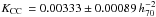 M⊙-1 and
 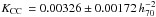 M⊙-1) suggest a lower number of CC SNe per unit mass of the parent stellar generation and, as a consequence, a narrow mass range for CC SN progenitors. The discrepancy between measurements of KCC in different volumes is connected to the difficulty in matching CC SN rate and SFR at higher redshifts that we discussed in the Sect. 5.
Appendix C: CC SN rate per unit luminosity and mass
The CC SN rate is proportional to the number of progenitor stars in a galaxy and hence to its SFR. When no information about SFR is available, a CC SN rate measurement in a galaxy sample can be normalised to some parameter related to the SFR, such as the total luminosity in an opportune band.
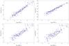 |
Fig. C.1 The LB, LK, LTIR and galaxy mass as a function of SFRUV in the sample C. |
The B band luminosity has been for a long time the only available parameter to normalise the SN rates in nearby galaxies (SNu unit10). The CC SN rate normalised per unit B band luminosity shows a strong dependence on the galaxy morphological type (Tammann 1974; Cappellaro et al. 1999) since the B band luminosity is the result of the combined effects of the emission by both old and young stellar populations and their relative contributions change along the Hubble sequence. A different tracer of the population of massive stars is provided by the TIR luminosity since a good correlation between SN rate and LTIRhas been observed (Cappellaro et al. 1999; Mannucci et al. 2003) but measurements were available only for a small sample of galaxies until few years ago.
Whereas B band luminosity is un-specific to the stellar age the luminosity in a reddish band, such as K band, is good tracer of the old population in a galaxy and therefore of the mean age of the stellar population. The combination of the K band luminosity and the B − K colour can be used as an indicator of the galaxy mass in star (Bell & de Jong 2001). The data collected from 2MASS allowed Mannucci et al. (2005) to normalise the SN rates in a sub-sample of Cappellaro et al. (1999) per unit K band luminosity and per unit galaxy mass by using the relation of Bell & de Jong (2001) and adopting a diet Salpeter.
We stress that the CC SN rate is related to the current SFR and not to the total stellar mass in a galaxy, while the type Ia SN rate is expected to be proportional to the K band luminosity and the galaxy mass so the normalisation per unit mass has a different meaning for different SN types. The relation between LB, LK, LTIR, mass and SFR for the galaxies in the sample C is illustrated in Fig. C.1 and a detailed discussion about the expected type Ia SN rate as a function of the galaxy luminosity and colours can be find in Greggio (2010).
According to the estimated rates in Cappellaro et al. (1999) and the total LB in our galaxy samples we expect to observe 14 ± 4, 12 ± 3, 9 ± 3 CC SNe for the sample A, B and C compared to the 14, 13 and 12 discovered in the last 13 years, while according to the total LK and galaxy mass in our sample C and the CC SN rates from Mannucci et al. (2005) we expect to observe 7 ± 2 and 13 ± 2 CC SNe respectively compared to the 12 discovered in the last 13 years. We found a good agreement between the expected and observed number of CC SNe both for rate normalised per unit luminosity and per unit mass, i.e. there is no discrepancy in the number of CC SNe detected within the 11 HUGS galaxy sample and the rate of CC SNe within z ~ < 0.01. The expected number of type Ia SNe in 13 years by adopting the rate estimate by Cappellaro et al. (1999) and the B band luminosity of our galaxy sample A is 4 ± 1. The probability of finding only 1 or 0 type Ia SN is ~9%.
It is interesting to compare the observed volumetric CC SN rate, (2 ± 0.5) × 10-4 Mpc-3 yr-1, within 11 Mpc with that expected by assuming a luminosity density or a SFR density. If we adopted a B band luminosity density jB = 1.03 × 10⁸ LB, ⊙ Mpc-3 obtained by fitting several measurements in the redshift interval 0 < z < 1 as in Botticella et al. (2008) the expected CC SN rate is rCC = 0.8 ± 0.2 × 10⁻⁴ Mpc-3 yr-1 a factor two lower than the observed value. However, if we normalise the CC SN rate per unit B band luminosity there is a perfect consistency between the values within 11 Mpc and z < 0.01 (Cappellaro et al. 1999).
Beacom (2010) estimated a CC SN rate of (1.25 ± 0.25) × 10-4 Mpc-3 yr-1 at redshift 0 from the cosmic SFR density measurements assuming a Salpeter IMF, a mass range between 8–50 M⊙ and H0 = 70 km s-1 Mpc-1. This estimate becomes (1.02 ± 0.25) × 10-4 Mpc-3 yr-1 if we adopt H0 = 75 km s-1 Mpc-1 and it is still a factor two lower than the observed value. Horiuchi et al. (2011) adopted a SFR density of 0.017 M⊙ Mpc-3 yr-1 for H0 = 73 km s-1 Mpc-1 that becomes 0.018 M⊙ Mpc-3 yr-1H0 = 75 km s-1 Mpc-1 obtaining a CC SN rate of 1.5 × 10⁻⁴ Mpc-3 yr-1. The luminosity density estimate jB is independent of the SFR measurements used by Beacom (2010) and Horiuchi et al. (2011).
In both cases the difference between expected and observed rates is due to the local galaxy over-density: the SFR and luminosity density estimated in the Universe averaged over larger volumes do not trace the galaxy density within 11 Mpc. Karachentsev et al. (2004) found that the local luminosity density exceeds about 2 times the global density in spite of the presence of the Local Void11. The galaxy content also differs significantly from that in a larger volume since 11 of the 19 largest galaxies within 8 Mpc are near pure disks (Karachentsev et al. 2004). As a consequence, the cumulative distribution of the discovered SNe since 1998 as a function of distance does not follow the expected distribution in a growing volume.
Appendix D: CC SN rate as a function of galaxy properties
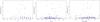 |
Fig. D.1 The SFRUV as a function of the morphological type, B − K and sSFR in the sample C. |
The number of the galaxies and CC SNe discovered in the last 13 years, the total SFRs, the CC SN rate, the total LB and LK, the CC SN rates normalised per unit luminosity and mass in galaxy sub-samples of the sample C based on morphological type, B − K colour, mass, sSFR and EW(Hα).
We expect that CC SN rate has a dependence on some galaxy properties related to the SFR (Fig. D.1) and the trend is different for different normalizations. In order to investigate some possible dependence we divided our galaxy sample C into sub-samples based on galaxy morphological type, B − K colour, mass, sSFR and EW(Hα) and measured the CC SN rate in each sub-sample (Table D.1).
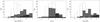 |
Fig. D.2 The distribution of the SFR, B − K colour and mass in the sub-samples with 0 ≤ T < 4 (black histogram), 4 ≤ T ≤ 7 (grey histogram) and the T > 7 (empty histogram) |
Morphology
It is well known that the morphological type sequence, in a first approximation, corresponds to a sequence in the SFR. We split each galaxy sample in four different sub-samples based on the galaxy RC3 type (Table D.1). The distribution of the SFR, B − K and mass in the 0 ≤ T < 4, 4 ≤ T ≤ 7 and the T > 7 sub-samples are illustrated in Fig. D.2. There is a statistically significant number of both galaxies and CC SNe only in the 4 ≤ T ≤ 7 sub-samples with 30% of galaxies and 80% of CC SNe, as expected. The total SFRHα and SFRUV in this sub-sample are about 75% of the total value in the sample C, while the CC SN rate is  yr-1 (Table D.1). To compare our result with that from Cappellaro et al. (1999) we assumed that the T < 0, 0 ≤ T < 4, 4 ≤ T ≤ 7 and the T > 7 sub-samples correspond to E–S0, S0a–Sb, Sbc–Sd and “Other” in the Cappellaro et al. (1999) sample, respectively. The CC SN rate in the sub-sample 4 ≤ T ≤ 7 has the value of
  SNu for the sample C that are in nice agreement with the value of 1.0 ± 0.4 SNu from Cappellaro et al. (1999).
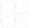 |
Fig. D.3 From the top to the bottom: the total SFRUV, the CC SN rate, the total LB, LK and mass in different sub-samples based on the galaxy morphological type. |
Our result is also consistent with that from LOSS of about SNu12 (Li et al. 2011a). The CC SN rate normalised per unit K band luminosity and mass in the sub-sample 4 ≤ T ≤ 7 has the value of SNuK and SNuM, respectively. Mannucci et al. (2005) estimated a CC SN rate of  SNuK and
  SNuM unit in Sbc–Sd galaxies, while Li et al. (2011a) estimated about
  SNuK13 and about
  SNuM14. Both the values from Mannucci et al. (2005) and Li et al. (2011a) are consistent with our estimates, the CC SN rate normalised per K band luminosity is slightly lower but the difference is not statistically significant.
The CC SN rate, the total LB, LK and mass in the different sub-samples 0 ≤ T < 4, 4 ≤ T ≤ 7 and the T > 7 are illustrated in the Fig. D.3.
B − K
An alternative indicator of the SFR are galaxy colours. Cappellaro et al. (1999) analysed for the first time the dependance of CC SN rates in SNu unit on the galaxy U − V colour pointing out that the CC SN rate is higher in the bluer galaxies. The strong dependence of the CC SN rates normalised per unit K band luminosity and unit mass on the galaxy B − K colour has been showed by Mannucci et al. (2005). Li et al. (2011a) found a very similar trend of the CC SN rates as a function of galaxy B − K colour: an increase from red to the blue galaxies. We considered two different bins in B − K colour (B − K ≤ 3 mag and B − K > 3 mag) with about the 80% and the 20% of CC SNe and galaxies, respectively (Table D.1). The total SFR (based on LHα and LFUV) and the total LB are higher in bluer galaxies while the total LK and total mass are larger in redder galaxies. The CC SN rates normalised per unit luminosity and mass are an order of magnitude higher in the bluer galaxies. There is a trend depending on the normalisation, increasing from SNu to SNuM as expected (Table D.1 and Fig. D.5).
Mass
There are several recent works probing the dependence of the SFR, sSFR and SF efficiency as a function of the stellar mass and suggesting that stellar mass plays a fundamental role in determining the fate of a galaxy (e.g. Schiminovich et al. 2007, 2010). The environment seems to be a second order effect compared with the mass. To analyse the CC SN rate as a function of the galaxy mass we split our galaxy sample in two sub-samples by using a cut of 5 × 10¹⁰ M⊙. In this case we have in the first sub-sample the 90% and 75% of the galaxies and CC SNe, respectively (Table D.1). The SFRHα, SFRUV and LB are similar in both sub-samples while the CC SN rates normalised per unit luminosity and mass are lower for the most massive galaxies (Table D.1 and Fig. D.5). If we split the sample C in two sub-samples by measuring the same total mass (about 93 × 1010 M⊙) we have the 95% of galaxies, the 84% of CC SNe, the 70% of SFRUV, the 65% of LB in the first sample. The CC SN rates are  and
and  SNu, and
  SNuK,
SNuK,  and
and  SNuM in the first and second sub-sample, respectively. With a different choice of the two sub-samples the difference between rates is lower.
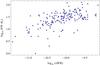 |
Fig. D.4 The EW(Hα) as a function of the sSFR in the sample C. |
sSFR and EW(Hα) We also measured the CC SN rate in two different galaxy sub-samples obtained by assuming a cut value of 10-10 yr-1 in sSFR (Table D.1) and found that about the 70% of CC SNe is in the galaxies with higher sSFR (44%). The fraction of total SFR (based on LHα and LFUV) in each sub-sample has similar values while LK and total mass are larger in galaxies with lower sSFR. The CC SN rates normalised per unit luminosity and mass are an order of magnitude higher in galaxies with lower sSFR. There is a trend depending on the normalisation, increasing from SNu to SNuM (Table D.1 and Fig. D.5).
 |
Fig. D.5 From the top to the bottom: the CC SN rates in SNu unit (left), SNuK unit (center) and SNuM unit (right) as a function of B − K, mass, sSFR and EW(Hα) respectively. |
We stress that the sSFR is tightly connected to the CC SN rate normalised per unit mass due to the relation between CC SN rate and SFR. EW(Hα) is an indicator of the sSFR so a tightly correlation between the sSFR, estimated by using the relation between galaxy mass, B − K colour and LK, and EW(Hα) is expected (Fig. D.4). It is also interesting to investigate the correlation between CC SN rate and EW(Hα) as done for the first time by Kennicutt (1984) for 171 galaxies and 55 SNe (11 of type II) that found a linear relation, supporting the massive star origin of the CC SN progenitors. We divided the galaxies in the sample C with measured EW(Hα) in two sub-samples by adopting a cut of 30 Å, that roughly corresponds to the same cut adopted in sSFR, and we found as expected very similar results (Table D.1 and Fig. D.4). If we split the sample C in two sub-samples by measuring the same total sSFR (about 1 × 10⁻⁸ yr-1) we have the 80% of galaxies, the 83% of CC SNe, the 80% of SFRUV, the 88% of LB in the first sample. The CC SN rates are and  SNu,
SNu,  and
and  SNuK,
SNuK,  and
and  SNuM in the first and second sub-sample, respectively.
All Tables
Number of galaxies and CC SNe discovered in the last 13 years, the total LHα, LB and SFR for the three samples we have analysed.
SN type, SN magnitude at the discovery epoch and at maximum light, phase (days) between the discovery epoch and the maximum light for the CC SNe discovered within 11 Mpc in the last 13 years, the host galaxy’s name, morphological type, B band absolute magnitude, SFRs (M⊙ yr-1), B − K colour, mass (1010 M⊙), specific SFR (yr-1) and EW(Hα).
Estimated minimum mass of CC SN progenitors in different galaxy samples derived considering a control time of 13 years and different assumptions about the number of CC SNe discovered in the last 13 years, the maximum mass for progenitors of CC SNe with optical signature, the IMF and the distance scale.
Fraction of galaxies, B band luminosity and discovered SNe in three different regions of the sky.
The number of the galaxies and CC SNe discovered in the last 13 years, the total SFR based on LHα and LFUV, the CC SN rate (RCC), the ratio between CC SN rate and SFR (KCC) and the total LB, LK and mass in different sub-samples based on SFRs.
The number of the galaxies and CC SNe discovered in the last 13 years, the total SFRs, the CC SN rate, the total LB and LK, the CC SN rates normalised per unit luminosity and mass in galaxy sub-samples of the sample C based on morphological type, B − K colour, mass, sSFR and EW(Hα).
All Figures
|
Fig. 1 The three galaxy samples selected for our analysis with the numbers of galaxies and discovered CC SNe in the last 13 years. |
| In the text | |
|
Fig. 2 Distribution of LHα (left panel) and LB (right panel), corrected for extinction, in the sample A (empty histogram), sample B (gray histogram) and sample C (black histogram). |
| In the text | |
|
Fig. 3 The observed light curves of different unreddened CC SN sub-types at 11 Mpc. The absolute magnitudes in R band at maximum are –19.16 mag for type Ia SNe, –17.92 mag for type Ib SNe, –16.38 mag for type IIP SNe, –17.70 mag for type IIL SNe and –17.14 mag for type IIn SNe. Phases are relative to the maximum epochs. |
| In the text | |
|
Fig. 4 The distribution of the discovery epoch with respect to the maximum light, of the discovery magnitude and absolute magnitude at maximum for our SN sample. The values for each CC SN and sources are reported in Table 2. |
| In the text | |
|
Fig. 5 The distribution of the LB, LK (in LB, ⊙ and LK, ⊙ unit), SFRs, B − K, mass, specific SFR and EW(Hα) for the galaxies that hosted SNe (full histogram) and all the galaxies (empty histogram) in the sample C. |
| In the text | |
|
Fig. 6 From the top to the bottom: the SFR expected from the CC SN rate in the sample A, B and C (thin lines) as a function of the upper mass limit for CC SN progenitors. We adopted a lower mass for CC SN progenitors of 8 M⊙. We plot the central value and 1σ confidence limits. The short dashed line indicates the value of SFR based on LHα (in all panels: sample A, B and C), the short dashed line the SFR based on LFUV (middle and bottom panels: samples B and C) and long dashed line the SFR based on LHα + LTIR (bottom panel: sample C). |
| In the text | |
|
Fig. 7 Probability density function of |
| In the text | |
|
Fig. 8 Posterior probability density function for |
| In the text | |
|
Fig. 9 The sky distribution of the galaxies in our sample A (red points). Blue points represent the galaxies that hosted CC SNe. The dimension of points is proportional to the CC SN number. |
| In the text | |
|
Fig. 10 The discovery rate of CC SNe from 1990 to 2009. The thick, dashed and thin lines are for CC SNe discovered in the whole Universe, within 60 Mpc and within 11 Mpc, respectively. |
| In the text | |
|
Fig. C.1 The LB, LK, LTIR and galaxy mass as a function of SFRUV in the sample C. |
| In the text | |
|
Fig. D.1 The SFRUV as a function of the morphological type, B − K and sSFR in the sample C. |
| In the text | |
|
Fig. D.2 The distribution of the SFR, B − K colour and mass in the sub-samples with 0 ≤ T < 4 (black histogram), 4 ≤ T ≤ 7 (grey histogram) and the T > 7 (empty histogram) |
| In the text | |
|
Fig. D.3 From the top to the bottom: the total SFRUV, the CC SN rate, the total LB, LK and mass in different sub-samples based on the galaxy morphological type. |
| In the text | |
|
Fig. D.4 The EW(Hα) as a function of the sSFR in the sample C. |
| In the text | |
|
Fig. D.5 From the top to the bottom: the CC SN rates in SNu unit (left), SNuK unit (center) and SNuM unit (right) as a function of B − K, mass, sSFR and EW(Hα) respectively. |
| In the text | |
Current usage metrics show cumulative count of Article Views (full-text article views including HTML views, PDF and ePub downloads, according to the available data) and Abstracts Views on Vision4Press platform.
Data correspond to usage on the plateform after 2015. The current usage metrics is available 48-96 hours after online publication and is updated daily on week days.
Initial download of the metrics may take a while.