© ESO, 2012

1. Introduction

The emission of some blazars is observed from radio frequencies up to VHE gamma rays. Collating observations from different energy ranges, we can show that the spectra of these objects contain two characteristic peaks (in νF(ν) plots). The first peak appears in the X-rays from a few keVs to a few hundred keVs and the second peak is observed around an energy of a few TeVs (e.g., Ghisellini et al. 1998, 2010; Massaro et al. 2004; Nieppola et al. 2006; Abdo et al. 2010b). Since the TeV emission is the most prominent feature in those sources we often call them TeV blazars, which constitutes a relatively small group of sources within the blazar family. The gamma-ray emission of most blazars peaks in the MeV − GeV range. Moreover, TeV gamma rays are efficiently absorbed by the EBL. This in addition limits the number of observed TeV blazars.

The high energy emission of blazars is believed to originate inside their jets. However, the observed variability on timescales from days (e.g., Catanese et al. 1997; Fossati et al. 2008) down to a few minutes (e.g., Aharonian et al. 2007a) indicates that only a small part of a jet is radiating at high energies. This kind of emission requires high energy particles, which can gain energy by acceleration at the front of a shock wave inside the jet. This is the simplest explanation of the acceleration process, which assumes that a small fraction of the jet bulk kinetic energy is transferred to the particles. In the presence of a magnetic field, the particles can radiate this energy through synchrotron emission, generating the first peak in the spectrum. Some fraction of the synchrotron photons can then be up-scattered to higher energies. This is the inverse-Compton (IC) scattering that gives the second peak in the TeV energies. This simple scenario has been proposed many times as part of models of the VHE emission of blazars (e.g., Dermer et al. 1997; Bloom & Marscher 1996; Inoue & Takahara 1996; Mastichiadis & Kirk 1997; Katarzyński et al. 2001).

A TeV gamma ray photon travelling through the intergalactic medium can interact with an infra-red photon producing an electron-positron pair. This causes absorption of the emission above a few hundred GeVs. To calculate this absorption, we have to determine the level of the intergalactic radiation field, which is difficult to measure directly but can be estimated from simulations of star light production in evolving galaxies. There are many different solutions for the level of the absorption (e.g., De Jager & Stecker 2002; Keneiste et al. 2004; Franceschini et al. 2008; Kneiske & Dole 2010). Thus the slope of the intrinsic TeV emission cannot be accurately calculated. Nevertheless, the TeV emission of some relatively distant sources (e.g., 1ES 1101-232 z = 0.186, Aharonian et al. 2006; or 1ES 0229+200, z = 0.14, Aharonian et al. 2007b) indicates that the intrinsic spectra are hard (F ∝ ν ^− α with 0.5 < α < 1), even if we assume as low as possible absorption.

It is difficult to explain how these hard spectra could be created. Most of the standard emission models assume a power-law or broken power-law particle energy distribution with a slope n ≃ 2 (where the number of particles N ∝ γ ^− n) and a minimum energy equivalent to γ_m ≃ 1. This gives the spectral index of the synchrotron emission α = (n − 1)/2 = 0.5. This emission is up-scattered to higher energies by the same population of the particles, hence the index of the inverse-Compton spectrum should be similar to the index of the synchrotron emission. Note that high energy particles (γ ≳ 10⁵) do not scatter efficiently because of the Klein-Nishina (KN) restrictions. The broken power-law particle distribution (n₁ and n₂ below and above the break, respectively) implies that there is a broken synchrotron spectrum (α₁ and α₂), for which the spectral index in the KN regime is approximately α ≃ 2α₂ − α₁ = 2.5 for n₂ = 4 (Tavecchio et al. 1998).

A question to ask is how we can explain the hard spectra from MeVs up to TeV gamma rays. One of the simplest solution is to assume a cut-off in the low energy part of the electron spectrum, which basically means γ_m  ≫  1. This solution was proposed for the first time by Katarzynski et al. (2006a) to explain the observations of 1ES 1101-232 in the TeV range. This cut-off leads to an additional break in the synchrotron spectrum between IR and X-ray energies. The spectral index of the first part of the spectrum, from radio up to X-ray energies, becomes a constant α₀ =  −1/3. This is a “tail” of the synchrotron emission produced by the low energy particles. This part of the radiation field with such a hard spectral index can also be up-scattered. Therefore, the IC spectrum can also be very hard up to limiting value α =  −1/3. Simultaneous optical and X-ray observations of 1ES 0229+200 performed by the Swift satellite (Tavecchio et al. 2009) shows an abrupt break between the optical and the X-ray range. This strongly implies that there is a low energy cut-off to the particle energy distribution.

In the present work, we explore this idea of a low energy cut-off. We focus on the unabsorbed MeV − GeV range where the spectral index of the intrinsic emission is observed directly. We demonstrate how to estimate the basic parameters of a source and how to explain the observed spectra by a simulation of the particle energy evolution. We apply our estimations and modelling to the X-ray and gamma-ray observations of two blazars with known redshifts.

2. Observations

The spectra of TeV blazars in the MeV−GeV range are always hard with spectral indices α < 1. The average expected value of the spectral index in this particular range is α ~ 0.5. In this work we focus on the sources with α < 0.5 that we call exceptionally hard.

For all blazars observed by the Fermi Gamma-ray Space Telescope (Atwood et al. 2009) from 20 MeV up to 300 GeV, only in some cases were spectra published in the Fermi Large Area Telescope First Source Catalog (Abdo et al. 2010a) exceptionally hard with the photon index Γ ≲ 1.5 (where the photon index is greater by unity in comparison to the spectral index). Moreover, in many cases we either do not know the distance to the observed sources (e.g. RBS 158 Γ = 1.34  ±  0.33, RBS 621 Γ = 1.42  ±  0.32) or the spectra were obtained with a relatively large uncertainty (e.g. 1ES 1101-232 Γ = 1.36  ±  0.58). Therefore, we selected only two objects for our test.

The observational parameters of the first object RGB J0710+591 (z = 0.125) in the Fermi catalogue are Γ = 1.28  ±  0.22, and F = (1.46 ± 0.49)  ×  10^-11 erg cm^-2 s^-1, where F is the energy flux in the 100 MeV to 100 GeV range. This source was also discovered by the VERITAS gamma-ray observatory in the TeV range (Acciari et al. 2010). The photon index obtained by VERITAS above  ~300 GeV was Γ = 2.69  ±  46. In our analysis, we also use X-ray observations obtained by the Swift satellite in the energy range from 0.2 to 10 keV (Acciari et al. 2010). A notable characteristic of this object is that the X-ray peak is observed at the level a few times higher than the GeV-TeV peak. This indicates that the synchrotron cooling is dominating in this source.

The photon index of the second source 1ES 0502+675 (z = 0.341) in the Fermi catalogue is rather soft Γ = 1.75  ±  0.11. However, the MeV − GeV spectrum of this source is quite complex. Owing the limited photon statistics, the observations published by Abdo et al. (2010b,c) seem to display a broken power-law spectrum of IC emission. This is rather unexpected and not predicted by any model of blazar emission. However, this may have a simple explanation if we assume for example that two independent jet components were observed at the same time. The break in the spectrum appears around an energy of 1 GeV. Fitting a single power-law function to the observations above this energy, we obtained Γ = 1.35  ±  0.20 and Γ = 1.46  ±  0.18 for the data sets above quoted, respectively. The VERITAS team reported the detection of this source in the TeV energy range (Ong 2009). However, no public information about the observed flux and slope has been publicly available so far. In addition we use quasi-simultaneous observations from Swift (Abdo et al. 2010b). The comparison between the X-ray peak level and the GeV observations shows that in this particular source the radiative cooling generated by the IC emission is the predominant cooling process.

3. Estimations

To estimate the basic parameters of a source of VHE emission, we adapted approach proposed by Tavecchio et al. (1998). We assume a spherical source of radius R, filled uniformly by a constant magnetic field (B) and relativistic particles (K – density). In addition, we assume that the particle energy distribution is a broken power-law (n₁,n₂,γ_b – break energy) and that the source travels with relativistic velocity (δ – Doppler factor) inside a jet. Finally, we included a low energy cut-off in the particle energy spectrum (γ_m – minimum energy). This is our main extension to the initial approach that let us estimate the basic physical parameters from the exceptionally hard spectrum. Even this simple scenario has eight free parameters. Therefore, using observational quantities we can only estimate the relation between the main parameters B and δ. However, we can estimate this relation in four different ways.

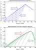Fig. 1 Approximate synchrotron and IC spectra calculated for different values of γm, from almost unity up to γb. This test demonstrates how the spectral index in the MeV − GeV range depends on the γm value. The dashed line shows the difference between the estimated (α1 = 0.5) and calculated (α ≃ 0.65) spectral slope below the peak.

3.1. Peak positions

The simplest estimation of the B − δ relation involves the comparison of the synchrotron peak position (ν_s) with the inverse-Compton peak frequency (ν_c). The positions of the peaks do not depend on γ_m thus we can directly use the formula derived by Tavecchio et al. (1998) $\mathit{B}\mathrm{=}\mathrm{(}\mathrm{1}\mathrm{+}\mathit{z}\mathrm{)}\frac{{\mathit{\nu }}_{\mathrm{s}}^{\mathrm{2}}}{\mathrm{2.8}\mathrm{\times }{\mathrm{10}}^{\mathrm{6}}{\mathit{\nu }}_{\mathrm{c}}}{\mathit{\delta }}^{-1}\mathit{.}$(1)In Fig. 1, we illustrate how an approximate IC spectrum evolve with time for different values of γ_m, from γ_m ≳ 1 up to γ_b. The spectra are calculated according to the prescription given in the Appendix. This simple test shows that the IC peak remains at the same position for the wide range of γ_m values with the exception for γ_m ≃ γ_b and this gives the limit to the above formula. The IC spectrum with α =  −1/3 that could be obtained for γ_m = γ_b was never observed directly. The observed spectral indices described in the previous section are in range from 0.3 to 0.5. Therefore, we can safely use this B and δ relationship for our estimations.

The spectra in Fig. 1 were calculated for n₁ = 2 and n₂ = 4, which directly gives the spectral indices of the synchrotron emission below (α₁ = 0.5) and above (α₂ = 3/2) the peak, respectively. The value of n₁ = 2 is rather typical for many different astrophysical sources. This may be the result of the first-order Fermi acceleration at a shock front or the synchrotron or the inverse-Compton cooling in the Thompson regime. This index is crucial for the emission of TeV blazars because this part of the particle spectrum provides synchrotron photons for the IC scattering. The IC spectrum in the MeV − GeV range comes mostly from the scattering in the Thompson regime. Therefore, the spectral index of this emission should be similar to the index of the scattered radiation field. However, the complexity of the scattering (see Fig. A.1) produces a curved spectrum below the peak. In the MeV − GeV range, just below the peak, the spectrum can be approximated well by a power-law function with the index α ≃ 0.65. This differs significantly from the estimated value α = 0.5 that is clearly illustrated in Fig. 1. Note that this concerns only the case where γ_m ~ 1 because γ_m controls the slope in the other cases. Since the somewhat classical value of n₁ = 2, postulated by many different particle evolution scenarios, gives α = 0.65 all spectra with α < 0.65 should be classified as exceptionally hard. Using this revised criterion, all spectra considered here may be regarded as exceptionally hard.

3.2. Peak levels

The second relationship between B and δ derived by Tavecchio et al. (1998) was obtained from the well-known formula $\frac{{\mathit{U}}_{\mathrm{syn}}}{{\mathit{U}}_{\mathit{B}}}\mathrm{=}\frac{{\mathit{L}}_{\mathrm{c}}}{{\mathit{L}}_{\mathrm{s}}}\mathit{,}$(2)where U_syn and U_B are the energy densities of the synchrotron radiation field and the magnetic field, respectively, and L_s and L_c are the total luminosities of the synchrotron and the IC emission, respectively. The luminosities were calculated from the observed spectral slopes and the peak emission levels. Unfortunately, we cannot adopt this approach in our estimations because usually we do not observe the break in the synchrotron emission (ν_m) that is related to γ_m. We instead compare $\frac{{\mathit{j}}_{\mathrm{c}}\mathrm{\left(}{\mathit{\nu }}_{\mathrm{c}}^{\mathrm{\prime }}\mathrm{\right)}}{{\mathit{j}}_{\mathrm{s}}\mathrm{\left(}{\mathit{\nu }}_{\mathrm{s}}^{\mathrm{\prime }}\mathrm{\right)}}\mathrm{=}\frac{{\mathit{F}}_{\mathrm{c}}\mathrm{\left(}{\mathit{\nu }}_{\mathrm{c}}\mathrm{\right)}}{{\mathit{F}}_{\mathrm{s}}\mathrm{\left(}{\mathit{\nu }}_{\mathrm{s}}\mathrm{\right)}}$(3)the emissivities (Eqs. (A.2), (B.1)) with the observed emission levels at the peaks. This gives the particle density (Eq. (B.2)) for the first part of the particle energy distribution ${\mathit{K}}_{\mathrm{1}}\mathrm{=}\frac{\mathrm{\left(}{\mathit{x}}_{\mathrm{s}}^{\mathrm{\prime }}{\mathrm{)}}^{\mathrm{-}{\mathit{\alpha }}_{\mathrm{1}}}{\mathit{F}}_{\mathrm{c}}\mathrm{\right(}{\mathit{\nu }}_{\mathrm{c}}\mathrm{)}}{{\mathit{j}}_{\mathrm{c}\mathit{,}\mathrm{sim}}\mathrm{\left(}{\mathit{x}}_{\mathrm{c}}^{\mathrm{\prime }}\mathrm{\right)}{\mathit{F}}_{\mathrm{s}}\mathrm{\left(}{\mathit{\nu }}_{\mathrm{s}}\mathrm{\right)}}\mathit{,}$(4)where $\begin{array}{ccc}{\mathit{j}}_{\mathrm{c}\mathit{,}\mathrm{sim}}\mathrm{\left(}{\mathit{x}}^{\mathrm{\prime }}\mathrm{\right)}& \mathrm{=}& \frac{{\mathit{\sigma }}_{\mathrm{T}}\mathit{R}}{\mathrm{4}}\{{\left(\frac{\mathrm{3}{\mathit{x}}^{\mathrm{\prime }}}{\mathrm{4}}\right)}^{\mathrm{-}{\mathit{\alpha }}_{\mathrm{1}}}\ln \left(\frac{{\mathit{\gamma }}_{\mathrm{b}}^{\mathrm{2}}}{\mathrm{(}{\mathit{x}}^{\mathrm{\prime }}{\mathrm{)}}^{\mathrm{2}}}\right)\\ & & \mathrm{+}\hspace{0.17em}\frac{{\mathit{\gamma }}_{\mathrm{b}}^{{\mathit{n}}_{\mathrm{2}}\mathrm{-}{\mathit{n}}_{\mathrm{1}}}}{{\mathit{\alpha }}_{\mathrm{2}}\mathrm{-}{\mathit{\alpha }}_{\mathrm{1}}}{\left(\frac{\mathrm{3}{\mathit{x}}^{\mathrm{\prime }}}{\mathrm{4}}\right)}^{\mathrm{-}{\mathit{\alpha }}_{\mathrm{2}}}{\left(\frac{\mathrm{3}{\mathit{x}}^{\mathrm{\prime }}}{\mathrm{4}{\mathit{\gamma }}_{\mathrm{b}}}\right)}^{{\mathit{\alpha }}_{\mathrm{2}}\mathrm{-}{\mathit{\alpha }}_{\mathrm{1}}}\begin{array}{}\mathrm{⎫}\\ \mathrm{⎪}\\ \mathrm{⎪}\\ \mathrm{⎬}\\ \mathrm{⎪}\\ \mathrm{⎪}\\ \mathrm{⎭}\end{array}\end{array}$(5)is the simplified version of the IC emissivity calculated as a sum of two dominant components j_c,sim = j_(1,1) + j_(1,2) (Eqs. (B.8), (B.9)). Note that in the component j_(1,2) the lower integration boundary was neglected. Finally, using the synchrotron emissivity (Eq. (A.2)) and the transformation given by Eq. (A.5) we can derive another relation between B and δ$\mathit{B}\mathrm{=}{\begin{array}{}\mathrm{⎧}\\ \mathrm{⎪}\\ \mathrm{⎪}\\ \mathrm{⎨}\\ \mathrm{⎪}\\ \mathrm{⎪}\\ \mathrm{⎩}\end{array}\frac{\frac{\mathrm{1}}{\mathrm{3}}\mathit{C}\mathrm{\left(}{\mathit{n}}_{\mathrm{1}}\mathrm{\right)}\mathrm{(}\mathrm{1}\mathrm{+}\mathit{z}\mathrm{)}{\mathit{R}}^{\mathrm{3}}{\mathit{K}}_{\mathrm{1}}{\mathit{\nu }}_{\mathrm{s}}^{\mathrm{-}{\mathit{\alpha }}_{\mathrm{1}}}}{{\mathit{F}}_{\mathrm{s}}\mathrm{\left(}{\mathit{\nu }}_{\mathrm{s}}\mathrm{\right)}{\mathit{D}}_{\mathit{L}}^{\mathrm{2}}}\begin{array}{}\mathrm{⎫}\\ \mathrm{⎪}\\ \mathrm{⎪}\\ \mathrm{⎬}\\ \mathrm{⎪}\\ \mathrm{⎪}\\ \mathrm{⎭}\end{array}}^{\frac{\mathrm{1}}{\mathrm{-}\mathrm{1}\mathrm{-}{\mathit{\alpha }}_{\mathrm{1}}}}{\mathit{\delta }}^{\frac{\mathrm{3}}{\mathrm{-}\mathrm{1}\mathrm{-}{\mathit{\alpha }}_{\mathrm{1}}}}\mathit{,}$(6)where the luminosity distance (D_L) is calculated in a ΛCDM universe for h = 0.72, Ω_Λ = 0.7, and Ω_m = 0.3 for all estimations and the spectra calculated in this work.

3.3. Spectral index in MeV–GeV range

Another constraint on the basic physical parameters can be obtained from the slope of the gamma-ray emission in the MeV–GeV range. This constraint assumes that the particle minimal energy (γ_m) is directly related to the radiative cooling inside the source. This is one of the main assumptions in our model that we discuss in detail in the next section. According to this assumption ${\mathit{\gamma }}_{\mathrm{m}}\mathrm{=}\frac{\mathrm{3}{\mathit{m}}_{\mathrm{e}}{\mathit{c}}^{\mathrm{2}}}{\mathrm{4}{\mathit{\sigma }}_{\mathrm{T}}\mathit{c}{\mathit{t}}_{\mathrm{cool}}\mathrm{(}{\mathit{U}}_{\mathit{B}}\mathrm{+}{\mathit{U}}_{\mathrm{syn}}\mathrm{)}}\mathit{,}$(7)where t_cool is the characteristic cooling time equivalent to the source evolution time in this particular case. This and the synchrotron energy density (U_syn) are unknown parameters. Therefore, for our estimation we assume that U_syn = x_BU_B is energy independent and can be parametrized as some fraction (x_B) of U_B. In the same way, we parametrize t_cool = x_RR/c as the multiplied crossing time. Since the spectral peaks are observed at almost the same level we may conclude that x_B ~ 1. In addition, we know that x_R must be greater than unity, although, in our estimations we assume that x_R ≥ 2. This gives the shortest reasonable time for the source evolution. With the above assumptions, we can derive an upper limit to the magnetic field value $\mathit{B}\mathrm{\le }\sqrt{\frac{\mathrm{3}{\mathit{m}}_{\mathrm{e}}{\mathit{c}}^{\mathrm{2}}\mathit{\pi }}{\mathrm{2}{\mathit{\sigma }}_{\mathrm{T}}\mathit{R}{\mathit{\gamma }}_{\mathrm{m}}}}\mathit{,}$(8)where γ_m value required by the above formula can be obtained from the spectral slope in the MeV − GeV range. However, there is no simple analytic formula that gives γ_m.

We derive the the minimum energy (γ_m) generating spectra from γ_m = 1 up to γ_m = γ_b and searching for the required spectral index $\mathit{\alpha }\mathrm{=}\frac{\ln \mathrm{\left(}{\mathit{j}}_{\mathrm{c}}\mathrm{\right(}{\mathit{\nu }}_{\mathrm{2}}^{\mathrm{\prime }}\mathrm{)}\mathit{/}{\mathit{j}}_{\mathrm{c}}\mathrm{(}{\mathit{\nu }}_{\mathrm{1}}^{\mathrm{\prime }}{\mathrm{\left)}}^{\mathrm{\right)}}}{\ln \mathrm{(}{\mathit{\nu }}_{\mathrm{1}}^{\mathrm{\prime }}\mathit{/}{{\mathit{\nu }}_{\mathrm{2}}^{\mathrm{\prime }}}^{\mathrm{)}}}\mathit{,}$(9)where ${\mathit{\nu }}_{\mathrm{1}}^{\mathrm{\prime }}$ and ${\mathit{\nu }}_{\mathrm{2}}^{\mathrm{\prime }}$ are the corresponding frequencies to the energies 100 MeV and 100 GeV, respectively, in the comoving frame. The frequency transformation, which is required for this calculation, introduces the Doppler factor dependency into the estimation. Note that it is necessary to use the full emissivity (Eq. (B.1)) for this particular estimation. The emissivity can be calculated for any non-zero value of R,B, and K because the absolute level of the emission is unimportant in this calculation. Finally, to calculate the emissivity we need the energy spectrum break that is given by a simple formula ${\mathit{\gamma }}_{\mathrm{b}}\mathrm{=}{\mathit{x}}_{\mathrm{c}}^{\mathrm{\prime }}\exp \left(\frac{\mathrm{1}}{\mathrm{2}\mathrm{(}{\mathit{\alpha }}_{\mathrm{2}}\mathrm{-}{\mathit{\alpha }}_{\mathrm{1}}\mathrm{)}}\mathrm{-}\frac{\mathrm{1}}{{\mathit{\alpha }}_{\mathrm{1}}\mathrm{-}\mathrm{1}}\right)$(10)derived by Tavecchio et al. (1998).

3.4. Pair absorption

The optical depth for the pair absorption inside a spherical source can be approximated as $\mathit{\tau }\mathrm{\left(}{\mathit{x}}_{\mathrm{0}}^{\mathrm{\prime }}\mathrm{\right)}\mathrm{=}\frac{\mathrm{1}}{\mathrm{5}}{\mathit{\sigma }}_{\mathrm{T}}{\mathit{n}}_{\mathrm{s}}\mathrm{\left(}{\mathit{x}}_{\mathrm{0}}^{\mathrm{\prime }}\mathrm{\right)}{\mathit{x}}_{\mathrm{0}}^{\mathrm{\prime }}\mathrm{2}\mathit{R,}$(11)where ${\mathit{n}}_{\mathrm{s}}\mathrm{=}\mathrm{3}\mathit{\pi }{\mathit{j}}_{\mathrm{s}}\mathit{R}\mathit{/}\mathrm{\left(}\mathit{hc}{\mathit{x}}_{\mathrm{0}}^{\mathrm{\prime }}\mathrm{\right)}$ is the number density of soft photons per energy interval (e.g., Coppi & Blandford 1990). The above formula incorporates a simple relation between the soft photon and the gamma-ray photon energy ${\mathit{x}}_{\mathrm{0}}^{\mathrm{\prime }}\mathrm{=}\mathrm{1}\mathit{/}{\mathit{x}}^{\mathrm{\prime }}$. Using the flux transformation (Eq. (A.5)), we can write $\mathit{\tau }\mathrm{=}\frac{\mathrm{9}}{\mathrm{10}}\frac{{\mathit{\sigma }}_{\mathrm{T}}{\mathit{F}}_{\mathrm{s}}\mathrm{\left(}{\mathit{\nu }}_{\mathrm{0}}\mathrm{\right)}{\mathit{D}}_{\mathit{L}}^{\mathrm{2}}}{{\mathit{\delta }}^{\mathrm{3}}\mathrm{(}\mathrm{1}\mathrm{+}\mathit{z}\mathrm{)}\mathit{Rhc}}\mathit{,}$(12)which should be smaller than unity for an optically thin source. This gives a lower limit to the value of the Doppler factor $\mathit{\delta }\mathrm{\ge }{\left[\frac{\mathrm{9}}{\mathrm{10}}\frac{{\mathit{\sigma }}_{\mathrm{T}}\mathrm{(}\mathrm{1}\mathrm{+}\mathit{z}{\mathrm{)}}^{\mathrm{2}{\mathit{\alpha }}_{\mathrm{1}}\mathrm{-}\mathrm{1}}{\mathit{F}}_{\mathrm{s}}\mathrm{(}{\mathit{\nu }}_{\mathrm{0}}\mathrm{)}{\mathit{D}}_{\mathit{L}}^{\mathrm{2}}}{\mathit{Rhc}}\right]}^{\frac{\mathrm{1}}{\mathrm{2}{\mathit{\alpha }}_{\mathrm{1}}\mathrm{+}\mathrm{3}}}\mathit{,}$(13)where ν₀ = (m_ec²/h)²/ν_c. Note that this formula is more accurate for a spherical source than the relationship derived by Dondi & Ghisellini (1995) used in the paper by Tavecchio et al. (1998). Our formula infers a lower limit that is almost five times higher than the above quoted relationship.

3.5. Estimation results

It is difficult to determine the position of the peaks in RGB J0710+591 from the available observations. The Swift energy range is quite narrow and the gamma-ray observations made by Fermi and VERITAS are not simultaneous. We analysed therefore two alternative solutions focusing first on the Swift and Fermi observations and then using the Swift and VERITAS data with different assumption about the peak positions.

To estimate the basic physical parameters of RGB J0710+591 we assume both the position of the synchrotron peak (ν_s = 7  ×  10¹⁷ Hz) and the emission level at the peak (ν_sF_s(ν_s) = 3  ×  10^-11 erg cm² s^-1). It is also necessary to assume the frequency of the IC peak (ν_c = 9.5  ×  10²⁵ Hz) and the emission level at this peak (ν_cF_c(ν_c) = 10^-11 erg cm² s^-1). However, for this peak we assume additional discrepancy of about  ± 30% in both the position and the emission level as well. This discrepancy is introduced because of the unknown extragalactic absorption. The spectral index of the synchrotron emission below the peak is assumed to be α₁ = 0.5 (n₁ = 2), whereas above the peak we use α₂ = 3/2 (n₂ = 4).

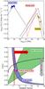Fig. 2 The upper panel shows the high energy emission of RGB J0710+591 and approximated spectra used for our estimations. In the lower panel, we illustrate the constraints to the basic parameters obtained in four different ways and the values selected for the modelling.

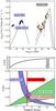Fig. 3 The upper panel shows the multi-frequency emission of 1ES 0502+675 observed by the Swift & Fermi instruments (Abdo et al. 2010b – squares; Abdo et al. 2010c – circles) and the approximate spectra used for the estimation presented in the lower panel. The values of B and δ selected for our modelling are indicated by the dot.

With the above assumptions, we can estimate the values of B and δ in the four different ways described in the previous subsections. The spectra used for the estimation and the estimation result are presented in Fig. 2. On the basis of the constraints obtained from the peak positions (Eq. (1)) and the emission levels (Eq. (6)), we found two crossing areas because of the discrepancy in the IC peak. The two other methods provide upper limit to the magnetic field value and the lower limit to the Doppler factor.

To calculate some of the limiting curves, we have to determine the radius of the emitting region. This parameter in principle can be constrained from the observed variability timescales R ≲ ct_varδ/(1 + z). However, there is no information about the variability of RGB J0710+591. We therefore selected as large as possible a value of the radius R = 2  ×  10¹⁶ cm, which still provides a good agreement for the four different estimation methods.

In the second approach, we focus on the VERITAS observations of RGB J0710+591 assuming that the IC peak is at the frequency ν_c = 2  ×  10²⁶ Hz and the emission level at this peak is ν_cF_c(ν_c) = 9.5  ×  10^-12 erg cm² s^-1. In addition me must assume that the synchrotron peak is placed above the observed range (ν_s = 3  ×  10¹⁸ Hz and ν_sF_s(ν_s) = 4  ×  10^-11 erg cm² s^-1). This assumption is similar to the solution proposed by Acciari et al. (2010) that helps us to explain a “flat” (Γ ~ 2) intrinsic TeV spectrum.

In the case of 1ES 0502+675, we assumed the same parameters for the synchrotron peak as for RGB J0710+591 and that ν_c = 2.5  ×  10²⁶ Hz, and ν_cF_c(ν_c) = 1.5  ×  10^-10 erg cm² s^-1 for the IC peak. Moreover, we used α₁ = 0.375 (n₁ = 1.75) and α₂ = 2 (n₂ = 5). We explain this particular choice in the next section.

The main difference between this estimation and the calculations performed for RGB J0710+591 is in the upper limit to the magnetic field obtained from the spectral slope in the MeV–GeV range. This estimate was calculated under the assumption that x_B ≃ 1 (U_syn ≃ U_B). However, the observations indicate that the emission at the IC peak, in this particular source, might even be one order of magnitude higher than the emission at the synchrotron peak. This would indicate that x_B  ≫  1 but a more precise value of this parameter cannot be estimated from the observations because the IC scattering at the peak is already in the Klein-Nishina regime. This illustrates a limitation of this particular estimation method. Finally, we selected as large as possible radius (R = 10¹⁶ cm), which provided a good agreement between our four different methods of the estimation.

4. Modelling

The information that we can obtain from the analysed observations is significantly limited. We therefore decided to apply quite simple model of the emission that is directly related to our estimation methods. The basic assumptions of the model that we adopted are identical to the assumptions made for the estimations. The VHE originates in a spherical source uniformly filled by relativistic particles and an entangled magnetic field. The source evolves in time, “fresh” particles are continuously injected into the source where they lose energy by means of the synchrotron and the IC emission. This is a simple adaptation of the jet internal shock model, where the particles efficiently accelerated at a shock front fill the downstream region of the shock.

The evolution of the particle energy spectrum inside the source is described by the kinetic equation $\frac{\mathit{\partial N}\mathrm{\left(}\mathit{\gamma ,t}\mathrm{\right)}}{\mathit{\partial t}}\mathrm{+}\frac{\mathit{\partial }}{\mathit{\partial \gamma }}\mathrm{\left[}\mathrm{\{}\mathit{\gamma ̇}\mathrm{syn}\mathrm{+}\mathit{\gamma ̇}{\mathrm{IC}}^{\mathrm{\}}}\mathit{N}\mathrm{\right(}\mathit{\gamma ,t}{\mathrm{\left)}}^{\mathrm{\right]}}\mathrm{=}\mathit{Q}\mathrm{\left(}\mathit{\gamma }\mathrm{\right)}\mathrm{+}\mathit{P}\mathrm{\left(}\mathit{\gamma ,t}\mathrm{\right)}\mathit{,}$(14)where is the synchrotron cooling rate and the IC cooling rate () is calculated according to the prescription of Sauge & Henri (2004) for an isotropic distribution of soft photons, using the full Klein-Nishina cross-section in the head-on approximation (Jones 1968). The injection rate is described by a power-law function $\mathit{Q}\mathrm{\left(}\mathit{\gamma }\mathrm{\right)}\mathrm{=}{\mathit{Q}}_{\mathrm{0}}{\mathit{\gamma }}^{\mathrm{-}{\mathit{n}}_{\mathit{i}}}\mathrm{for}\mathit{\gamma }\mathrm{\ge }{\mathit{\gamma }}_{\mathit{i}}\mathit{,}$(15)where γ_i ≫ 1 describes the minimum energy of the injected particles. Finally, we simulate the pair creation process within the source, where the pair injection rate P(γ,t) is calculated using the approach described by Sauge & Henri (2004). This process in principle should be negligible when we use the parameters obtained from our estimations. However, in the estimation our intention was to use as large as possible a radius that gives a relatively small value of the Doppler factor. The value is only slightly larger than the lower limit obtained from our simple estimation (Eq. (13)). Therefore, the pair creation process may have a small impact on the evolution of the particle energy spectrum in our more precise simulation. To solve the kinetic equation, we used the numerical method described by Chiaberge & Ghisellini (1999). Calculating spectra for each time step, we are carefully checked the energetic balance between the injected and radiated energy.

Such simple time-dependent modelling has been already proposed many times to explain evolution of the TeV blazars emission (e.g., Dermer et al. 1999; Kusunose et al. 2000; Böttcher & Chiang 2002; Sauge & Henri 2004). The main difference between our approach and the other models is in the minimum injected energy, where in the other approaches γ_i = 1 is usually assumed. In other words, we assume that the acceleration process at the shock front is very efficient and “pushes” almost all particles towards high relativistic energies. This is somehow similar to the formation of either a thermal or quasi-thermal particle energy distribution (e.g., Schlickeiser 1984; Katarzyński et al. 2006b).

To obtain an exceptionally hard spectrum in the MeV − GeV range, we needed to apply a cut-off to the low energy part of the spectrum. This cut-off can be produced in a natural way by the radiative cooling. Injecting only high energy particles, we may obtain a broken power-law particle distribution with the break at the γ_i energy. The minimum energy (γ_m) that the particles can reach in the source evolution time is given by Eq. (7) (e.g., Kardashev 1962). This shows that in principle, the particles might cool down to γ ~ 1, if the source evolution is long enough. However, the minimum energy is inversely proportional to time, which means that the high energy particles (γ ~ 10⁵) lose energy more rapidly than the medium energy particles (γ ~ 10³). Moreover, in the downstream region of the shock there may be another acceleration process, for example a turbulent second-order Fermi acceleration. This relatively weak process may not produce any high energy activity but it can be strong enough to compensate at some point for the radiative cooling and to keep the minimum energy significantly above the particle rest energy. This is, however, a much more complex approach that requires an analysis of possible activity. With no information about time-dependent flux variations, we simply assume that the source evolution time is just 2R/c.

The spectral index of the particle energy spectrum below the break will be constant n₁ = 2, whereas above the peak the index depends on the injection slope n₂ = n_i + 1. This, however, is true only for the radiative cooling caused by either the synchrotron emission or the IC emission in the Thompson regime. In the Klein-Nishina regime, the scattering efficiency of the high energy particles is significantly lower. This modifies the high energy part of the energy distribution (e.g., Moderski et al. 2005). It is difficult to describe this effect analytically in our particular scenario. We may perform only a simple estimation assuming that the energy density of the synchrotron radiation field is given by ${\mathit{U}}_{\mathrm{syn}}\mathrm{\simeq }\frac{\mathrm{4}\mathit{\pi }}{\mathit{c}}{\mathrm{\int }}_{{\mathit{\nu }}_{\mathrm{1}}^{\mathrm{\prime }}}^{{\mathit{\nu }}_{\mathrm{2}}^{\mathrm{\prime }}}{\mathit{I}}_{\mathrm{s}}\mathrm{\left(}{\mathit{\nu }}^{\mathrm{\prime }}\mathrm{\right)}\mathrm{d}{\mathit{\nu }}^{\mathrm{\prime }}\mathit{,}$(16)where ${\mathit{\nu }}_{\mathrm{1}}^{\mathrm{\prime }}$ is the minimum frequency of the scattered photons and ${\mathit{\nu }}_{\mathrm{2}}^{\mathrm{\prime }}\mathrm{=}\min \mathrm{[}{\mathit{\nu }}_{\mathit{x}}^{\mathrm{\prime }}\mathit{,}\mathrm{3}{\mathit{m}}_{\mathrm{e}}{\mathit{c}}^{\mathrm{2}}\mathit{/}\mathrm{(}\mathrm{4}\mathit{h\gamma }\mathrm{\left)}\mathrm{\right]}$ introduces the KN restriction in a simple form (e.g., Chiaberge & Ghisellini 1999). Neglecting the lower boundary in the above integral and assuming that ${\mathit{\nu }}_{\mathrm{2}}^{\mathrm{\prime }}\mathrm{=}\mathrm{3}{\mathit{m}}_{\mathrm{e}}{\mathit{c}}^{\mathrm{2}}\mathit{/}\mathrm{\left(}\mathrm{4}\mathit{h\gamma }\mathrm{\right)}$ and I_s ∝ (ν′) ^− α₁, we may approximate the IC cooling ratio as . Hence, the stationary (Ṅ = 0) solution of the kinetic equation is given by N ∝ γ ^{− 2 − α₁}, where the slope is significantly lower than the value N ∝ γ^-2 obtained for a constant classical synchrotron or IC cooling. This agrees with our more precise numerical tests, which indicate that the radiative cooling dominated by the IC scattering in the KN regime can reduce the particle energy slope by a factor  ≲ 1/2. This appears to be true for the cooled (below the break) and injected (above the break) part of the energy spectrum. Since the emission of 1ES 0502+675 seems to be significantly affected by the scattering in the KN regime, we assume that n₁ = 1.75 for the estimation made in the previous section for this source. We note that the energy spectrum index less than two helps in addition to explain exceptionally hard MeV − GeV spectra.

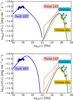Fig. 4 The modelling of the RGB J0710+591 spectral emission. The upper panel shows the first approach where we considered the Swift and Fermi observations only. In the lower panel, we demonstrate an alternative approach that can explain the origin of the TeV emission observed by VERITAS. Note that the Fermi and the VERITAS observations were not simultaneous. To obtain the observed IC spectra, we used the EBL lower-limit model proposed by Kneiske & Dole (2010), where the dashed lines show the intrinsic unabsorbed emission.

Figure 4 shows the modelling of the RGB J0710+591 emission. We present the results obtained for two different sets of physical parameters derived from the estimations performed in the previous section. Note that the IC spectrum obtained in the first case is unable to explain the intrinsic shape of the emission. In the second case, the intrinsic spectrum is reproduced well but the level of the MeV − GeV emission is significantly lower than the observed level. However, the Fermi and the VERITAS observations are not simultaneous, hence there may be a difference in the emission levels. The detailed values of the physical parameters used for the modelling are given in Table 1. There are only six important parameters illustrating the simplicity of the model. In addition, we assumed that the maximum Lorentz factor of the injected particles is γ > 10⁷ and the source evolution time t_evo = 2R/c.

For 1ES 0502+675, we do not attempt to reproduce the Swift UVOT observations. This part of the emission might be dominated by either the host galaxy or more extended jet structures as demonstrated for example in the case of Mrk 501 (Katarzynski et al. 2001). Moreover, no direct correlation between X-ray and optical variability in other TeV blazars also implies that the optical-UV emission has a different origin. Our modelling is also unable to explain the inverted spectral slope in the 100 MeV to 1 GeV energy range. This is an unexpected and puzzling feature of the emission that will require additional investigation.

However, this may be simply the IC emission produced by the extended jet structures, which also dominate the emission in the optical-UV range.

5. Summary

Several blazars observed by the Fermi Gamma-Ray Space Telescope have exceptionally hard spectra in the MeV − GeV range. We have demonstrated that in principle all sources with a spectral index α ≲ 0.65 should be classified as sources with an exceptionally hard MeV − GeV spectrum. Therefore, we have attempted to reproduce these spectral slopes by assuming a low energy cut-off in the particle energy distribution. This approach had been previously developed to explain hard spectra in the TeV range and at least in one case (1ES 0229+200 Tavecchio et al. 2009) it was found to be correct.

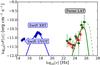Fig. 5 The spectra obtained from the modelling of 1ES 0502+675 for the physical parameters obtained from our estimation.

We derived four different methods to estimate the basic parameters of the emitting region. Three of these methods had been previously proposed and we simply adapted them to the case of the low energy cut-off. Our method that gives an upper limit to the magnetic field, derived from the spectral slope in the MeV–GeV range, was proposed here for the first time. This particular constraint can be very useful but it requires accurate measurements of the spectral index in the not-absorbed MeV–GeV range.

Finally, we used our modelling estimates that succeed to explain the exceptionally hard spectra in terms of particle energy evolution. Our model is relatively simple but more complex, and hence more accurate modelling would require far tighter observational constraints. We have attempted to explain the emission of two different TeV blazars. The particle evolution in RGB J0710+591 seems to be dominated by synchrotron cooling, whereas in 1ES 0502+675 IC cooling appears to dominate. In both cases, the estimated parameters of B and δ provide good results in our modelling. This type of modelling is crucial for understanding the nature of the blazar emission process, especially in non-standard cases such as the exceptionally hard MeV–GeV emission. One interpretation of exceptionally hard spectra is that for some reason only high energy particles can produce the X-ray and gamma-ray activity of TeV blazars.

Acknowledgments

We thank the anonymous referee for a careful review and a helpful report.

References

Appendix A: Approximation of synchrotron emission

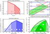Fig. A.1 An example of an approximation of SSC emission. The figure shows a broken power-law (γb) electron spectrum with a low energy cut-off (γm) that extends up to some maximal energy (γx). This distribution generates synchrotron emission with two breaks (${\mathit{\nu }}_{\mathrm{m}}^{\mathrm{\prime }}\mathit{,}{\mathit{\nu }}_{\mathrm{s}}^{\mathrm{\prime }}$) and extends from some minimal (${\mathit{\nu }}_{\mathit{l}}^{\mathrm{\prime }}$) to some maximal frequency (${\mathit{\nu }}_{\mathit{x}}^{\mathrm{\prime }}$). The energy spectrum is divided into two parts, whereas the synchrotron radiation is divided into three parts. This provides six different components of the inverse-Compton emission. Each component must be integrated with different boundary conditions. The upper right panel demonstrates how to choose these conditions. This panel shows synchrotron frequencies as functions of the IC photon frequencies, where the horizontal lines indicate the characteristic frequencies in the synchrotron spectrum. Three slanted lines are calculated according to the well-know relation ${\mathit{\nu }}_{\mathrm{IC}}^{\mathrm{\prime }}\mathrm{=}\mathrm{(}\mathrm{4}\mathit{/}\mathrm{3}\mathrm{)}{\mathit{\gamma }}^{\mathrm{2}}{\mathit{\nu }}_{\mathrm{syn}}^{\mathrm{\prime }}$ for the three characteristic particle energies (γm,γb,γx). The single opposite slanted line shows the Klein-Nishina restriction according to the approximation ${\mathit{x}}^{\mathrm{\prime }}\mathrm{=}\mathrm{3}\mathit{/}\mathrm{\left(}\mathrm{4}{\mathit{x}}_{\mathrm{0}}^{\mathrm{\prime }}\mathrm{\right)}$. The crossing lines produce six rectangle areas that indicate the lower and upper integration boundaries for each component. Each component of the IC emission is indicated by a pair of numbers where the first number refers to the part of the electron energy spectrum and the second number shows the part of the radiation field used to create this component.

For a power-law particle energy distribution $\mathit{N}\mathrm{\left(}\mathit{\gamma }\mathrm{\right)}\mathrm{=}\mathit{K}{\mathit{\gamma }}^{\mathrm{-}\mathit{n}}\mathit{,}\mathrm{\left[}{\mathrm{cm}}^{-3}\mathrm{\right]}$(A.1)the synchrotron emissivity can be approximated by a simple power-law function ${\mathit{j}}_{\mathrm{s}}\mathrm{\left(}{\mathit{\nu }}^{\mathrm{\prime }}\mathrm{\right)}\mathrm{=}\frac{\mathrm{1}}{\mathrm{4}\mathit{\pi }}\mathit{C}\mathrm{\left(}\mathit{n}\mathrm{\right)}\mathit{K}{\mathit{B}}^{\mathit{\alpha }\mathrm{+}\mathrm{1}}\mathrm{(}{\mathit{\nu }}^{\mathrm{\prime }}{\mathrm{)}}^{\mathrm{-}\mathit{\alpha }}\mathit{,}\hspace{0.17em}\mathrm{[}\mathrm{erg}\hspace{0.17em}{\mathrm{s}}^{-1}\hspace{0.17em}{\mathrm{cm}}^{-3}\hspace{0.17em}{\mathrm{sterad}}^{-1}\hspace{0.17em}{\mathrm{Hz}}^{-1}\mathrm{]}\mathit{,}$(A.2)where α = (n − 1)/2 and $\begin{array}{ccc}\mathit{C}\mathrm{\left(}\mathit{n}\mathrm{\right)}& \mathrm{=}& \frac{\mathrm{4}\sqrt{\mathrm{3}}\mathit{\pi }{\mathit{e}}^{\mathrm{3}}}{{\mathit{m}}_{\mathrm{e}}{\mathit{c}}^{\mathrm{2}}}{\left(\frac{\mathrm{3}\mathit{e}}{\mathrm{2}\mathit{\pi }{\mathit{m}}_{\mathrm{e}}\mathit{c}}\right)}^{\frac{\mathit{n}\mathrm{-}\mathrm{1}}{\mathrm{2}}}\mathrm{\Gamma }\left(\frac{\mathrm{3}\mathit{n}\mathrm{-}\mathrm{1}}{\mathrm{12}}\right)\mathrm{\Gamma }\left(\frac{\mathrm{3}\mathit{n}\mathrm{+}\mathrm{19}}{\mathrm{12}}\right)\\ & & \mathrm{\times }\hspace{0.17em}\mathrm{\Gamma }\left(\frac{\mathit{n}\mathrm{+}\mathrm{5}}{\mathrm{4}}\right)\mathit{/}\mathrm{(}\mathrm{8}\sqrt{\mathit{\pi }}\mathrm{(}\mathit{n}\mathrm{+}\mathrm{1}\mathrm{)}\mathrm{\Gamma }\mathrm{\left(}\mathrm{\right(}\mathit{n}\mathrm{+}\mathrm{7}\mathrm{)}\mathit{/}\mathrm{4}{\mathrm{)}}^{\mathrm{)}}\end{array}$(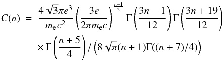A.3)(e.g., Ginzburg & Syrovatskii 1965). Assuming an optically thin source, we can write the synchrotron luminosity L_s = 4πVj_s [erg], where V is the source volume. If our source is spherical then the intensity of the surface emission is given by ${\mathit{I}}_{\mathrm{s}}\mathrm{=}\frac{\mathrm{4}}{\mathrm{3}}{\mathit{j}}_{\mathrm{s}}\mathit{R}\mathrm{[}\mathrm{erg}{\mathrm{s}}^{-1}{\mathrm{cm}}^{-2} {\mathrm{sterad}}^{-1} {\mathrm{Hz}}^{-1}\mathrm{]}\mathit{,}$(A.4)where R is the source radius. This gives L_s = 4π²R²I_s and using the standard luminosity-to-flux conversion, we can obtain the observed flux F_s = π(R/D_L)²I_s [erg cm^-2], where D_L is the luminosity distance. For relativistically moving sources at cosmological distances, we have to apply additional transformations to the flux ${\mathit{F}}_{\mathrm{s}}\mathrm{\left(}\mathit{\nu }\mathrm{\right)}\mathrm{=}\mathit{\pi }\frac{{\mathit{R}}^{\mathrm{2}}}{{\mathit{D}}_{\mathit{L}}^{\mathrm{2}}}\mathrm{(}\mathrm{1}\mathrm{+}\mathit{z}\mathrm{)}{\mathit{\delta }}^{\mathrm{3}}{\mathit{I}}_{\mathrm{s}}\mathrm{\left(}{\mathit{\nu }}^{\mathrm{\prime }}\mathrm{\right)}\mathit{,}$(A.5)as well as the frequency ν = ν′δ/(1 + z).

Appendix B: Approximation of inverse-Compton emission

The inverse-Compton emissivity can be approximated by a simple formula ${\mathit{j}}_{\mathrm{c}}\mathrm{\left(}{\mathit{x}}^{\mathrm{\prime }}\mathrm{\right)}\mathrm{=}\frac{{\mathit{\sigma }}_{\mathrm{T}}}{\mathrm{4}}{\mathrm{\int }}_{{\mathit{x}}_{\mathrm{1}}}^{{\mathit{x}}_{\mathrm{2}}}\mathit{N}\left(\sqrt{\frac{\mathrm{3}{\mathit{x}}^{\mathrm{\prime }}}{\mathrm{4}{\mathit{x}}_{\mathrm{0}}^{\mathrm{\prime }}}}\right)\sqrt{\frac{\mathrm{3}{\mathit{x}}^{\mathrm{\prime }}}{\mathrm{4}{\mathit{x}}_{\mathrm{0}}^{\mathrm{\prime }}}}\frac{{\mathit{I}}_{\mathrm{s}}\mathrm{\left(}{\mathit{x}}_{\mathrm{0}}^{\mathrm{\prime }}\mathrm{\right)}}{{\mathit{x}}_{\mathrm{0}}^{\mathrm{\prime }}}\mathrm{d}{\mathit{x}}_{\mathrm{0}}^{\mathrm{\prime }}\mathit{,}$(B.1)where x′ = hν′/m_ec² is the inverse-Compton photon energy normalized to the electron rest energy and ${\mathit{x}}_{\mathrm{0}}^{\mathrm{\prime }}$ is the energy of a synchrotron photon also divided by m_ec². The particle energy spectrum, in our particular estimations, is assumed to be a broken power-law 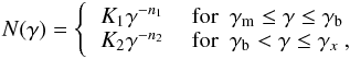$\mathit{N}\mathrm{\left(}\mathit{\gamma }\mathrm{\right)}\mathrm{=}\{\begin{array}{}\\ {\mathit{K}}_{\mathrm{1}}{\mathit{\gamma }}^{\mathrm{-}{\mathit{n}}_{\mathrm{1}}}\mathrm{for} {\mathit{\gamma }}_{\mathrm{m}}\mathrm{\le }\mathit{\gamma }\mathrm{\le }{\mathit{\gamma }}_{\mathrm{b}}\\ {\mathit{K}}_{\mathrm{2}}{\mathit{\gamma }}^{\mathrm{-}{\mathit{n}}_{\mathrm{2}}}\mathrm{for} {\mathit{\gamma }}_{\mathrm{b}}\mathit{<}\mathit{\gamma }\mathrm{\le }{\mathit{\gamma }}_{\mathit{x}}\mathrm{,}\end{array}$(B.2)where K₂ = K₁γ^{n₂ − n₁} and γ_m ≫ 1. For such an energy spectrum, we can approximate the synchrotron intensity by a double broken power-law function 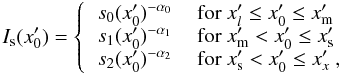${\mathit{I}}_{\mathrm{s}}\mathrm{\left(}{\mathit{x}}_{\mathrm{0}}^{\mathrm{\prime }}\mathrm{\right)}\mathrm{=}\{\begin{array}{}\\ {\mathit{s}}_{\mathrm{0}}\mathrm{(}{\mathit{x}}_{\mathrm{0}}^{\mathrm{\prime }}{\mathrm{)}}^{\mathrm{-}{\mathit{\alpha }}_{\mathrm{0}}}\mathrm{for}{\mathit{x}}_{\mathit{l}}^{\mathrm{\prime }}\mathrm{\le }{\mathit{x}}_{\mathrm{0}}^{\mathrm{\prime }}\mathrm{\le }{\mathit{x}}_{\mathrm{m}}^{\mathrm{\prime }}\\ {\mathit{s}}_{\mathrm{1}}\mathrm{(}{\mathit{x}}_{\mathrm{0}}^{\mathrm{\prime }}{\mathrm{)}}^{\mathrm{-}{\mathit{\alpha }}_{\mathrm{1}}}\mathrm{for}{\mathit{x}}_{\mathrm{m}}^{\mathrm{\prime }}\mathit{<}{\mathit{x}}_{\mathrm{0}}^{\mathrm{\prime }}\mathrm{\le }{\mathit{x}}_{\mathrm{s}}^{\mathrm{\prime }}\\ {\mathit{s}}_{\mathrm{2}}\mathrm{(}{\mathit{x}}_{\mathrm{0}}^{\mathrm{\prime }}{\mathrm{)}}^{\mathrm{-}{\mathit{\alpha }}_{\mathrm{2}}}\mathrm{for}{\mathit{x}}_{\mathrm{s}}^{\mathrm{\prime }}\mathit{<}{\mathit{x}}_{\mathrm{0}}^{\mathrm{\prime }}\mathrm{\le }{\mathit{x}}_{\mathit{x}}^{\mathrm{\prime }}\mathrm{,}\end{array}$(B.3)that extends from some minimal energy (${\mathit{x}}_{\mathit{l}}^{\mathrm{\prime }}$) up to the maximal energy (${\mathit{x}}_{\mathit{x}}^{\mathrm{\prime }}$) and contains breaks at the characteristic energies (${\mathit{x}}_{\mathrm{m}}^{\mathrm{\prime }}\mathit{,}{\mathit{x}}_{\mathrm{s}}^{\mathrm{\prime }}$) related to the particle energy by ${\mathit{x}}_{\mathrm{m}\mathit{/}\mathrm{s}}^{\mathrm{\prime }}\mathrm{=}\frac{\mathit{h}}{{\mathit{m}}_{\mathrm{e}}{\mathit{c}}^{\mathrm{2}}}\mathrm{3.7}\mathrm{\times }{\mathrm{10}}^{\mathrm{6}}{\mathit{\gamma }}_{\mathrm{m}\mathit{/}\mathrm{b}}^{\mathrm{2}}\mathit{B}\mathit{.}$(B.4)According to Eqs. (A.2) and (A.4), the normalizing coefficients in the synchrotron intensity are given by $\begin{array}{ccc}& & {\mathit{s}}_{\mathrm{1}\mathit{/}\mathrm{2}}\mathrm{=}\frac{\mathrm{1}}{\mathrm{4}\mathit{\pi }}\mathit{C}\mathrm{\left(}{\mathit{n}}_{\mathrm{1}\mathit{/}\mathrm{2}}\mathrm{\right)}{\left(\frac{{\mathit{m}}_{\mathrm{e}}{\mathit{c}}^{\mathrm{2}}}{\mathit{h}}\right)}^{\mathrm{-}{\mathit{\alpha }}_{\mathrm{1}\mathit{/}\mathrm{2}}}\mathit{R}{\mathit{K}}_{\mathrm{1}\mathit{/}\mathrm{2}}{\mathit{B}}^{{\mathit{\alpha }}_{\mathrm{1}\mathit{/}\mathrm{2}}\mathrm{+}\mathrm{1}}\mathit{,}\\ & & {\mathit{s}}_{\mathrm{0}}\mathrm{=}{\mathit{s}}_{\mathrm{1}}\mathrm{(}{\mathit{x}}_{\mathrm{m}}^{\mathrm{\prime }}{\mathrm{)}}^{{\mathit{\alpha }}_{\mathrm{0}}\mathrm{-}{\mathit{\alpha }}_{\mathrm{1}}}\mathit{.}\end{array}$\arraycolsep1.75ptNote that inside the source the intensity of the synchrotron radiation field is on average I_s ≃ (3/4)Rj_s (e.g., Kataoka et al. 1999). Therefore, there is no constant 4/3 in the above formulae.

Since the energy spectrum (Eq. (B.2)) and the radiation field spectrum (Eq. (B.3)) are divided into the simple power-law functions, we can split the inverse-Compton emissivity into six components where each component is described by ${\mathit{j}}_{\mathrm{\left(}\mathit{a,b}\mathrm{\right)}}\mathrm{\left(}{\mathit{x}}^{\mathrm{\prime }}\mathrm{\right)}\mathrm{=}\frac{{\mathit{\sigma }}_{\mathrm{T}}}{\mathrm{4}}{\mathit{s}}_{\mathit{b}}{\mathit{K}}_{\mathit{a}}{\left(\frac{\mathrm{3}{\mathit{x}}^{\mathrm{\prime }}}{\mathrm{4}}\right)}^{\frac{\mathrm{1}\mathrm{-}{\mathit{n}}_{\mathit{a}}}{\mathrm{2}}}{\mathrm{\int }}_{{\mathit{x}}_{\mathrm{1}}}^{{\mathit{x}}_{\mathrm{2}}}\mathrm{(}{\mathit{x}}_{\mathrm{0}}^{\mathrm{\prime }}{\mathrm{)}}^{\frac{{\mathit{n}}_{\mathit{a}}\mathrm{-}\mathrm{1}}{\mathrm{2}}\mathrm{-}\mathrm{1}\mathrm{-}{\mathit{\alpha }}_{\mathit{b}}}\mathrm{d}{\mathit{x}}_{\mathrm{0}}^{\mathrm{\prime }}\mathit{,}$(B.7)where index a (equal either to 1 or 2) describes parts of the particle energy spectrum and index b (equal 0, 1 or 2) indicates parts of the synchrotron spectrum. Depending on the a,b values, this gives two different results. For a = b, we have ${\mathit{j}}_{\mathrm{\left(}\mathit{a,a}\mathrm{\right)}}\mathrm{\left(}{\mathit{x}}^{\mathrm{\prime }}\mathrm{\right)}\mathrm{=}\frac{{\mathit{\sigma }}_{\mathrm{T}}}{\mathrm{4}}{\mathit{s}}_{\mathit{a}}{\mathit{K}}_{\mathit{a}}{\left(\frac{\mathrm{3}{\mathit{x}}^{\mathrm{\prime }}}{\mathrm{4}}\right)}^{\mathrm{-}{\mathit{\alpha }}_{\mathit{a}}}\ln \mathrm{(}{\mathit{x}}_{\mathrm{2}}\mathit{/}{\mathit{x}}_{\mathrm{1}}\mathrm{)}$(B.8)and for a ≠ b${\mathit{j}}_{\mathrm{\left(}\mathit{a,b}\mathrm{\right)}}\mathrm{\left(}{\mathit{x}}^{\mathrm{\prime }}\mathrm{\right)}\mathrm{=}\frac{{\mathit{\sigma }}_{\mathrm{T}}}{\mathrm{4}}{\mathit{s}}_{\mathit{b}}{\mathit{K}}_{\mathit{a}}{\left(\frac{\mathrm{3}{\mathit{x}}^{\mathrm{\prime }}}{\mathrm{4}}\right)}^{\mathrm{-}{\mathit{\alpha }}_{\mathit{a}}}\frac{{\mathit{x}}_{\mathrm{2}}^{{\mathit{\alpha }}_{\mathit{a}}}\mathrm{-}{\mathit{x}}_{\mathrm{1}}^{{\mathit{\alpha }}_{\mathit{b}}}}{{\mathit{\alpha }}_{\mathit{a}}\mathrm{-}{\mathit{\alpha }}_{\mathit{b}}}\mathrm{·}$(B.9)Finally, we have to define the integration boundaries (x₁,x₂), which are different for each component. In general, we can define the lower integration boundary as a maximum of two energies of synchrotron photons ${\mathit{x}}_{\mathrm{1}}\mathrm{=}\begin{array}{}\max \end{array}\mathrm{\left(}{\mathit{x}}_{\mathit{p}}^{\mathrm{\prime }}\mathit{,}{\mathit{x}}_{\mathit{q}}^{\mathrm{\prime }}\mathrm{\right)}\mathit{,}$(B.10)where ${\mathit{x}}_{\mathit{p}}^{\mathrm{\prime }}$ is equal to ${\mathit{x}}_{\mathit{l}}^{\mathrm{\prime }}\mathit{,}{\mathit{x}}_{\mathrm{m}}^{\mathrm{\prime }}$, or ${\mathit{x}}_{\mathrm{s}}^{\mathrm{\prime }}$ for b = 0,1,2, respectively, and ${\mathit{x}}_{\mathit{q}}^{\mathrm{\prime }}\mathrm{=}\mathrm{(}\mathrm{4}\mathit{/}\mathrm{3}\mathrm{)}{\mathit{\gamma }}^{\mathrm{2}}{\mathit{x}}_{\mathrm{0}}^{\mathrm{\prime }}$ is calculated for the characteristic particle energies γ_b,γ_x for a = 1 and 2, respectively. The upper boundary condition is calculated to be the minimum of three energies ${\mathit{x}}_{\mathrm{1}}\mathrm{=}\begin{array}{}\min \end{array}\left({\mathit{x}}_{\mathit{p}}^{\mathrm{\prime }}\mathit{,}{\mathit{x}}_{\mathit{q}}^{\mathrm{\prime }}\mathit{,}\frac{\mathrm{3}}{\mathrm{4}{\mathit{x}}^{\mathrm{\prime }}}\right)\mathit{,}$(B.11)where ${\mathit{x}}_{\mathit{p}}^{\mathrm{\prime }}$ is equal to either ${\mathit{x}}_{\mathrm{m}}^{\mathrm{\prime }}\mathit{,}{\mathit{x}}_{\mathrm{s}}^{\mathrm{\prime }}$, or ${\mathit{x}}_{\mathit{x}}^{\mathrm{\prime }}$ for b = 0,1,2, respectively and ${\mathit{x}}_{\mathit{q}}^{\mathrm{\prime }}$ is calculated for γ_m,γ_b for a = 1 and 2, respectively. The last part of this maximum comes from the simple approximation of the Klein-Nishina limit where ${\mathit{x}}^{\mathrm{\prime }}\mathrm{=}\frac{\mathrm{4}}{\mathrm{3}}{\mathit{\gamma }}^{\mathrm{2}}{\mathit{x}}_{\mathrm{0}}^{\mathrm{\prime }}\mathit{.}$(B.12)An example spectrum of the approximate IC emission and a description of the integration boundaries and the components

of the spectrum is presented in Fig. A.1. This particular spectrum was calculated for a set of the parameters that gives all six components of the spectrum. Note that for the parameters that are typical for TeV blazars, the IC scattering occurs predominantly in the KN regime and only two components (j_(1,1)) and (j_(2,1)) creates the spectrum if 1 ≪ γ_m ≪ γ_b. In the case where 1 ≪ γ_m ≃ γ_b, the first part of the energy spectrum (a = 1) and the second part of the radiation field (b = 1) basically do not exist. In such a case, the spectrum is dominated by the j_(2,0) component with the spectral index in the MeV − GeV range α₀ =  −1/3. However, this is an extreme limiting case, never directly observed.

All Tables

All Figures

	Fig. 1 Approximate synchrotron and IC spectra calculated for different values of γm, from almost unity up to γb. This test demonstrates how the spectral index in the MeV − GeV range depends on the γm value. The dashed line shows the difference between the estimated (α1 = 0.5) and calculated (α ≃ 0.65) spectral slope below the peak.
In the text

	Fig. 2 The upper panel shows the high energy emission of RGB J0710+591 and approximated spectra used for our estimations. In the lower panel, we illustrate the constraints to the basic parameters obtained in four different ways and the values selected for the modelling.
In the text

	Fig. 3 The upper panel shows the multi-frequency emission of 1ES 0502+675 observed by the Swift & Fermi instruments (Abdo et al. 2010b – squares; Abdo et al. 2010c – circles) and the approximate spectra used for the estimation presented in the lower panel. The values of B and δ selected for our modelling are indicated by the dot.
In the text

Fig. 4 The modelling of the RGB J0710+591 spectral emission. The upper panel shows the first approach where we considered the Swift and Fermi observations only. In the lower panel, we demonstrate an alternative approach that can explain the origin of the TeV emission observed by VERITAS. Note that the Fermi and the VERITAS observations were not simultaneous. To obtain the observed IC spectra, we used the EBL lower-limit model proposed by Kneiske & Dole (2010), where the dashed lines show the intrinsic unabsorbed emission.

In the text

	Fig. 5 The spectra obtained from the modelling of 1ES 0502+675 for the physical parameters obtained from our estimation.
In the text

Fig. A.1 An example of an approximation of SSC emission. The figure shows a broken power-law (γb) electron spectrum with a low energy cut-off (γm) that extends up to some maximal energy (γx). This distribution generates synchrotron emission with two breaks (${\mathit{\nu }}_{\mathrm{m}}^{\mathrm{\prime }}\mathit{,}{\mathit{\nu }}_{\mathrm{s}}^{\mathrm{\prime }}$) and extends from some minimal (${\mathit{\nu }}_{\mathit{l}}^{\mathrm{\prime }}$) to some maximal frequency (${\mathit{\nu }}_{\mathit{x}}^{\mathrm{\prime }}$). The energy spectrum is divided into two parts, whereas the synchrotron radiation is divided into three parts. This provides six different components of the inverse-Compton emission. Each component must be integrated with different boundary conditions. The upper right panel demonstrates how to choose these conditions. This panel shows synchrotron frequencies as functions of the IC photon frequencies, where the horizontal lines indicate the characteristic frequencies in the synchrotron spectrum. Three slanted lines are calculated according to the well-know relation ${\mathit{\nu }}_{\mathrm{IC}}^{\mathrm{\prime }}\mathrm{=}\mathrm{(}\mathrm{4}\mathit{/}\mathrm{3}\mathrm{)}{\mathit{\gamma }}^{\mathrm{2}}{\mathit{\nu }}_{\mathrm{syn}}^{\mathrm{\prime }}$ for the three characteristic particle energies (γm,γb,γx). The single opposite slanted line shows the Klein-Nishina restriction according to the approximation ${\mathit{x}}^{\mathrm{\prime }}\mathrm{=}\mathrm{3}\mathit{/}\mathrm{\left(}\mathrm{4}{\mathit{x}}_{\mathrm{0}}^{\mathrm{\prime }}\mathrm{\right)}$. The crossing lines produce six rectangle areas that indicate the lower and upper integration boundaries for each component. Each component of the IC emission is indicated by a pair of numbers where the first number refers to the part of the electron energy spectrum and the second number shows the part of the radiation field used to create this component.

In the text

References

- Abdo, A. A., Ackermann, M., Ajello, M., et al. 2010a, ApJS, 188, 405 [NASA ADS] [CrossRef] [Google Scholar]
- Abdo, A. A., Ackermann, M., Agudo, I., et al. 2010b, ApJ, 716, 30 [NASA ADS] [CrossRef] [Google Scholar]
- Abdo, A. A., Ackermann, M., Ajello, M., et al. 2010c, ApJ, 710, 1271 [NASA ADS] [CrossRef] [Google Scholar]
- Acciari, V. A., Aliu, E., Arlen, T., et al. 2010, ApJ, 715, L49 [NASA ADS] [CrossRef] [Google Scholar]
- Aharonian, F., Akhperjanian, A. G., Bazer-Bachi, A. R., et al. 2006, Nature, 440, 1018 [NASA ADS] [CrossRef] [PubMed] [Google Scholar]
- Aharonian, F., Akhperjanian, A. G., Bazer-Bachi, A. R., et al. 2007a, ApJ, 664, 71 [NASA ADS] [CrossRef] [Google Scholar]
- Aharonian, F., Akhperjanian, A. G., Barres de Almeida, U., et al. 2007b, A&A, 475, L9 [NASA ADS] [CrossRef] [EDP Sciences] [Google Scholar]
- Atwood, W. B., Abdo, A. A., Ackermann, M., et al. 2009, ApJ, 697, 1071 [NASA ADS] [CrossRef] [Google Scholar]
- Böttcher, M., & Chiang, J. 2002, ApJ, 581, 127 [NASA ADS] [CrossRef] [Google Scholar]
- Bloom, S. D., & Marscher, A. P. 1996, ApJ, 461, 657 [NASA ADS] [CrossRef] [Google Scholar]
- Catanese, M., Bradbury, S. M., Breslin, A. C., et al. 1997, ApJ, 487, L143 [NASA ADS] [CrossRef] [Google Scholar]
- Chiaberge, M., & Ghisellini, G. 1999, MNRAS, 306, 551 [NASA ADS] [CrossRef] [Google Scholar]
- Coppi, P. S., & Blandford, R. D. 1990, MNRAS, 245, 453 [NASA ADS] [Google Scholar]
- De Jager, O. C., & Stecker, F. W. 2002, 566, 738 [Google Scholar]
- Dermer, C. D., Sturner, S. J., & Schlickeiser, R. 1997, ApJS, 109, 103 [NASA ADS] [CrossRef] [Google Scholar]
- Dermer, C. D., Li, H., & Chiang, J. 1999, ApL&C, 39, 1 [Google Scholar]
- Dondi, L., & Ghisellini, G. 1995, MNRAS, 273, 583 [NASA ADS] [Google Scholar]
- Fossati, G., Buckley, J. H., Bond, I. H., et al. 2008, ApJ, 677, 906 [NASA ADS] [CrossRef] [Google Scholar]
- Franceschini, A., Rodighiero, G., & Vaccari, M. 2008, A&A, 487, 837 [NASA ADS] [CrossRef] [EDP Sciences] [Google Scholar]
- Ghisellini, G., Celotti, A., Fossati, G., et al. 1998, MNRAS, 301, 451 [NASA ADS] [CrossRef] [Google Scholar]
- Ghisellini, G., Tavecchio, F., Foschini, L., et al. 2010, MNRAS, 402, 497 [NASA ADS] [CrossRef] [Google Scholar]
- Ginzburg, V. L., & Syrovatskii, S. I. 1965, ARA&A, 3, 297 [NASA ADS] [CrossRef] [Google Scholar]
- Inoue, S., & Takahara, F. 1996, ApJ, 463, 555 [NASA ADS] [CrossRef] [Google Scholar]
- Jones, F. C. 1968, Phys. Rev., 167, 1159 [NASA ADS] [CrossRef] [Google Scholar]
- Massaro, E., Perri, M., Giommi, P., et al. 2004, A&A, 413, 489 [NASA ADS] [CrossRef] [EDP Sciences] [Google Scholar]
- Kardashev, N. S. 1962, SvA, 6, 317 [Google Scholar]
- Kataoka, J., Mattox, J. R., Quinn, J., et al. 1999, ApJ, 514, 138 [NASA ADS] [CrossRef] [Google Scholar]
- Katarzyński, K., Sol, H., & Kus, A. 2001, A&A, 367, 809 [NASA ADS] [CrossRef] [EDP Sciences] [Google Scholar]
- Katarzynski, K., Ghisellini, G., Tavecchio, F., et al. 2006a, MNRAS, 368, 52 [Google Scholar]
- Katarzynski, K., Ghisellini, G., Mastichiadis, A., et al. 2006b, A&A, 453, 47 [NASA ADS] [CrossRef] [EDP Sciences] [Google Scholar]
- Kneiske, T. M., & Dole, H. 2010, A&A, 515, A19 [NASA ADS] [CrossRef] [EDP Sciences] [Google Scholar]
- Kneiske, T. M., Bretz, T., Mannheim, K., & Hartmann, D. H. 2004, A&A, 413, 807 [NASA ADS] [CrossRef] [EDP Sciences] [Google Scholar]
- Kusunose, M., Takahara, F., & Li, H. 2000, ApJ, 536, 299 [NASA ADS] [CrossRef] [Google Scholar]
- Mastichiadis, A., & Kirk, J. 1997, A&A, 320, 19 [NASA ADS] [Google Scholar]
- Moderski, R., Sikora, M., Coppi, P. S., & Aharonian, F. 2005, MNRAS, 363, 954 [NASA ADS] [CrossRef] [Google Scholar]
- Nieppola, E., Tornikoski, M., & Valtaoja, E. 2006, A&A, 445, 441 [NASA ADS] [CrossRef] [EDP Sciences] [Google Scholar]
- Ong, R. A. 2009, ATel, 2301, 1O [NASA ADS] [Google Scholar]
- Sauge, L., & Henri, G. 2004, ApJ, 616, 136 [NASA ADS] [CrossRef] [Google Scholar]
- Schlickeiser, R. 1984, A&A, 136, 227 [NASA ADS] [Google Scholar]
- Tavecchio, F., Maraschi, L., & Ghisellini, G. 1998, ApJ, 509, 608 [NASA ADS] [CrossRef] [Google Scholar]
- Tavecchio, F., Ghisellini, G., Ghirlanda, G., et al. 2009, MNRAS, 399, 59 [Google Scholar]