| Issue |
A&A
Volume 682, February 2024
|
|
|---|---|---|
| Article Number | A134 | |
| Number of page(s) | 21 | |
| Section | Astrophysical processes | |
| DOI | https://doi.org/10.1051/0004-6361/202348121 | |
| Published online | 13 February 2024 | |
The variety of extreme blazars in the AstroSat view
1
Université Paris Cité, CNRS, Astroparticule et Cosmologie, 75013 Paris, France
e-mail: This email address is being protected from spambots. You need JavaScript enabled to view it.
2
Centre for Space Research, North-West University, Potchefstroom 2520, South Africa
3
Landessternwarte, Universität Heidelberg, Königstuhl 12, 69117 Heidelberg, Germany
e-mail: This email address is being protected from spambots. You need JavaScript enabled to view it.
4
Laboratoire Univers et Théories, Observatoire de Paris, Université PSL, CNRS, Université de Paris, 92190 Meudon, France
5
South African Astronomical Observatory, Observatory Road, Cape Town 7925, South Africa
6
Astronomical Observatory of Ivan Franko National University of Lviv, Kyryla i Methodia 8, 79005 Lviv, Ukraine
Received:
1
October
2023
Accepted:
17
November
2023
Abstract
Context. Among the blazar class, extreme blazars have exceptionally hard intrinsic X-ray/TeV spectra, and extreme peak energies in their spectral energy distribution (SED). Observational evidence suggests that the non-thermal emission from extreme blazars is typically non-variable. All these unique features present a challenging case for blazar emission models, especially regarding those sources with hard TeV spectra.
Aims. We aim to explore the X-ray and GeV observational features of a variety of extreme blazars, including extreme-TeV, extreme-synchrotron (extreme-Syn), and regular high-frequency-peaked BL Lac objects (HBLs). Furthermore, we aim to test the applicability of various blazar emission models that could explain the very hard TeV spectra.
Methods. We conducted a detailed spectral analysis of X-ray data collected with AstroSat and Swift-XRT, along with quasi-simultaneous γ-ray data from Fermi-LAT, for five sources: 1ES 0120+340, RGB J0710+591, 1ES 1101−232, 1ES 1741+196, and 1ES 2322−409. We took three approaches to modelling the SEDs: (1) a steady-state one-zone synchrotron-self-Compton (SSC) code, (2) another leptonic scenario of co-accelerated electrons and protons on multiple shocks applied to the extreme-TeV sources only (e–p co-acceleration scenario), and (3) a one-zone hadro-leptonic (ONEHALE) code. The latter code is used twice to explain the γ-ray emission process: proton synchrotron and synchrotron emission of secondary pairs.
Results. Our X-ray analysis provides well-constrained estimates of the synchrotron peak energies for both 1ES0120+340 and 1ES1741+196. These findings categorise these latter objects as extreme-synchrotron sources, as they consistently exhibit peak energies above 1 keV in different flux states. The multi-epoch X-ray and GeV data reveal spectral and flux variabilities in RGB J0710+591 and 1ES 1741+196, even on timescales of days to weeks. As anticipated, the one-zone SSC model adequately reproduces the SEDs of regular HBLs but encounters difficulties in explaining the hardest TeV emission. Hadronic models offer a reasonable fit to the hard TeV spectrum, though with the trade-off of requiring extreme jet powers. On the other hand, the lepto-hadronic scenario faces additional challenges in fitting the GeV spectra of extreme-TeV sources. Finally, the e–p co-acceleration scenario naturally accounts for the observed hard electron distributions and effectively matches the hardest TeV spectrum of RGB J0710+591 and 1ES 1101−232.
Key words: relativistic processes / galaxies: active / BL Lacertae objects: general
© The Authors 2024
 Open Access article, published by EDP Sciences, under the terms of the Creative Commons Attribution License (https://creativecommons.org/licenses/by/4.0), which permits unrestricted use, distribution, and reproduction in any medium, provided the original work is properly cited.
This article is published in open access under the Subscribe to Open model. This email address is being protected from spambots. You need JavaScript enabled to view it. to support open access publication.
1. Introduction
Blazars are a subclass of active galactic nuclei (AGN) that emit non-thermal, strongly polarised and variable continuum emission from a jet of relativistic plasma directed along or close to the line of sight (Blandford & Rees 1978; Urry & Padovani 1995). The broadband spectral energy distribution (SED) of blazars displays two broad humps: the low-energy emission (peaking in the submillimetre (submm) to soft X-ray range) is commonly ascribed to synchrotron emission from relativistic electrons in the jet, while the origin of the high-energy emission component (peaking at MeV to TeV energies) remains a subject of debate, with various proposed solutions (Abdo et al. 2010). Two viable scenarios, leptonic and hadronic, are widely used to explain the high-energy emission. Leptonic models propose that the high-energy emission comes from inverse Compton scattering of low-energy seed photons by ultrarelativistic leptons, either from the synchrotron radiation field in the emission region (synchrotron self-Compton, SSC; e.g, Ghisellini & Maraschi 1989; Bloom & Marscher 1996) or from photons originating external to the emission region (external Compton (EC); e.g. Dermer et al. 1992; Sikora et al. 1994). Hadronic models, on the other hand, assume that the high-energy emission originates from accelerated ultrarelativistic protons in the jet; through the proton synchrotron mechanism; or from secondary emission from particles such as electron–positron pairs or muons produced in pγ interactions (Mannheim & Biermann 1992; Mücke & Protheroe 2001; Böttcher et al. 2013).
Extreme high-synchrotron-peaked blazars (or eHBLs) a peculiar class of high-energy peaked blazars, pose a significant challenge to conventional blazar models because of their unique spectral characteristics (Costamante et al. 2001; Biteau et al. 2020 for a recent review). The eHBLs are typically characterised by an unusually hard intrinsic spectrum (photon index, Γ ∼ 1.5 − 1.9) in both their X-ray and very-high-energy (VHE) γ-ray emission, and their SED peaks at up to 1–10 keV (typically > 1 keV) in the synchrotron component, and a few TeV (> 1–10 TeV) in the high-energy component consistently in different flux states. It is worth noting that the extreme properties observed in these two energy bands do not always coexist, and the correlation between them remains unknown (Foffano et al. 2019; Costamante et al. 2018). Two types of blazars are recognised as being extreme: extreme synchrotron blazars (extreme-Syn; e.g. 1ES 0033+595, 1ES 0120+340) and extreme TeV blazars (extrem-TeV; e.g. 1ES 0229+200, 1ES 0347−121). However, these are distinct from transiting high-synchrotron-peaked blazars (HBLs), which only exhibit extreme behaviour during strong flares; examples being Mkn 421, Mkn 501, 1ES 1426+428, 1ES 2344+514, and 1ES 1959+650. In contrast, eHBLs are not known to show such strong flares and exhibit persistently extreme behaviour in different flux states.
Due to the low flux detectability and limited observational range in the X-ray and VHE γ-ray bands, there is still considerable uncertainty in locating the SED peak positions of extreme sources, and only a few have been identified so far. Several sources have been classified as extreme-Syn sources or potential sources based on BeppoSAX observations (Costamante et al. 2001), while a few have been confirmed by Costamante et al. (2018) through precise localisation of the synchrotron peak using joint XRT–NuSTAR observations. In the case of VHE γ-rays, the number of confirmed extreme sources is more than ten (Biteau et al. 2020; Acciari et al. 2020). Among the observed eHBLs, 1ES 0229+200 is the best example, displaying high peak frequencies in both X-rays and VHE γ-rays, and is therefore of great importance for jet physics, and for constraining important cosmological quantities such as the extragalactic background light and the intergalactic magnetic field (Aharonian et al. 2007a; Tavecchio et al. 2010; Bonnoli et al. 2015).
Unlike most TeV blazars, which exhibit significant fluctuations and flares, eHBLs appear to display relatively stable emissions. Despite the lack of strong flares or high flux activities on minute timescales at any wavelength, recent observations have indicated that moderate variability can be present in some eHBLs. For example, in X-rays, 1ES 1101−232 showed a variation of about 30% in flux and corresponding spectral variability (Wolter et al. 2000). The TeV light curve of 1ES 1218+304 exhibited rapid TeV variability over a few days, reaching approximately 20% of the Crab flux (Acciari et al. 2010b), while 1ES 0229+200 displayed moderate variations in TeV on timescales of about 1 yr (Aliu et al. 2014). These findings contradict the idea that the absence of variability is a universal feature of eHBLs.
A large variety of models that work within leptonic and hadronic scenarios have been proposed to explain the extreme emission. While a simple SSC model provides a good explanation for regular blazars and can also account for the extreme synchrotron emission observed in some sources, interpreting the extremely hard TeV spectrum within a purely leptonic SSC framework is challenging. This often requires a large minimum Lorentz factor (γmin ∼ 104 − 105; Katarzyński et al. 2006; Kaufmann et al. 2011) or hard particle spectra; as well as a very weak magnetic field (B ≤ 1 mG; Costamante et al. 2018). The limitations of the one-zone SSC model are widely discussed by Cerruti et al. (2015), Aguilar-Ruiz et al. (2022), and Biteau et al. (2020). Alternative approaches have been proposed to explain extreme TeV emission within the leptonic framework; for instance, an external Compton scenario, which involves the Compton upscattering of cosmic microwave background (CMB) photons in the extended kiloparsec(kpc)-scale jet (1ES 1101−232, Böttcher et al. 2008; Yan et al. 2012) and photons from the broad-line region (Lefa et al. 2011), or the internal γ-ray absorption scenario (Aharonian et al. 2008; Zacharopoulou et al. 2011). However, the short-term variability detected in some sources seems incompatible with such a kpc-scale-jet scenario. Another approach involves taking into account adiabatic losses or a Maxwellian-type electron distribution in a stochastic acceleration model, which leads to a very hard TeV spectrum (1ES 0229+200, Lefa et al. 2011).
In a recent work, Zech & Lemoine (2021) proposed a feasible solution to address the issues associated with the pure SSC model by providing more natural explanations for the requirement of large values of the minimum electron Lorentz factor and low magnetisation. The SSC model proposed by these latter authors is an extension of the standard SSC theory and assumes that both electron and proton populations are co-accelerated in relativistic internal or recollimation shocks. Possible energy-transfer mechanisms can naturally result in a very high value of γmin. The model considers different shock and recollimation scenarios that can explain extreme (ΓVHE ∼ 1.7 − 1.9; e.g. RGB J0710+591, 1ES 1101−232) to very extreme (ΓVHE ∼ 1.5, e.g., 1ES 0229+200) VHE γ-ray spectra and apparently require recollimation at more than a single shock to produce the hardest VHE spectra. Further, an adaptation of the Zech & Lemoine (2021) model was proposed by Tavecchio et al. (2022), where the extremely hard TeV emission is explained by a combination of recollimation and stochastic acceleration.
On the other hand, different flavours of hadronic models (proton synchrotron and secondary cascades produced in pγ interactions) have advantages over a standard leptonic model and somewhat relax the requirements for extreme parameter values. For instance, the lepto-hadronic solution suggested by Cerruti et al. (2015) effectively replicated an extremely hard TeV spectrum, albeit with a demand for hard injection functions. Another lepto-hadronic approach recently explored by Aguilar-Ruiz et al. (2022) suggested that the extreme emission comes from photo-hadronic interactions in a blob close to the AGN core and by SSC and external inverse Compton processes in an outer blob. Nevertheless, hadronic and lepto-hadronic models, in general, demand very high proton power, sometimes with super-Eddington values in the cases of extreme TeV sources. Li et al. (2022) devised a one-zone model based on hadronuclear (pp) interactions that circumvents extreme jet-power requirements.
In the present paper, we present recent observations carried out using AstroSat and Fermi-LAT of five sources: 1ES 0120+340 (redshift z = 0.272), RGB J0710+591 (z = 0.125), 1ES 1101–232 (z = 0.186), 1ES 1741+196 (z = 0.084), and 1ES 2322–409 (z = 0.1736), each displaying a unique range of spectral characteristics. Among these, RGB J0710+591 and 1ES 1101–232 are well-known for being extreme-TeV sources with hard intrinsic TeV spectra. Although TeV data are unavailable for 1ES 0120+340, this latter presents itself as a potential extreme-TeV candidate with hard X-ray and GeV spectra. Additionally, hints of an extreme-Syn nature can be seen in the XRT spectrum of 1ES 1741+196, while 1ES 2322–409 appears to be a standard HBL. The new sets of AstroSat and LAT data presented here reveal more detailed spectral and variability properties of these sources.
We conducted a detailed analysis of the SEDs of the selected sources using contemporaneous data obtained from AstroSat and Fermi-LAT in conjunction with archived data available in various energy bands (Sect. 2). We analysed the variability of the sources (Sect. 3) and modelled the various SEDs using different physical scenarios (Sect. 4). Firstly, we show how we used the one-zone SSC model developed by Böttcher et al. (2013), which has previously been successfully applied to a number of HBL sources. Secondly, we present our findings from the use of the electron–proton (e–p) co-acceleration model developed by Zech & Lemoine (2021) for certain extreme-TeV blazars. Lastly, we used the lepto-hadronic code ONEHALE (Zacharias 2021; Zacharias et al. 2022), which provides two different γ-ray emission solutions: one lepto-hadronic case dominated by emission from secondary pairs, and another purely hadronic case with γ-ray emission dominated by proton synchrotron. Further information regarding the model descriptions can be found in Appendix A. We present our conclusions in Sect. 5.
2. Observations and data analysis
We selected five HBL sources, 1ES 0120+340, RGB J0710+591, 1ES 1101–232, 1ES 1741+196, and 1ES 2322–409 for this work based on the available AstroSat data from our proposed observations. Four of them (all except 1ES 2322–409) are known to exhibit an eHBL nature. We analyse AstroSat and the contemporaneous Fermi-LAT data centred at the AstroSat observation periods. The Fermi-LAT data are averaged over 4–6 yr to attain a good fit statistic. The observation details are provided in Table 1 and the data analysis procedure is described in the following sections.
Details of the observations from various instruments of AstroSat missions.
2.1. AstroSat data: SXT, LAXPC, and UVIT
AstroSat is a multi-wavelength (MWL) space-based observatory that carries five scientific instruments on board covering a wide range of energies from UV to hard X-rays. The instruments used in this work are: the Large-Area X-ray Proportional Counters (LAXPCs), the Soft X-ray focusing Telescope (SXT), and the Ultraviolet Imaging Telescope (UVIT). SXT is a focusing telescope capable of X-ray imaging and spectroscopy in the energy range 0.3–8.0 keV (Singh et al. 2014, 2016, 2017). The LAXPC instrument consists of three proportional counter units (LAXPC10, LAXPC20 and LAXPC30), providing coverage in the 3–80 keV hard X-ray band (Yadav et al. 2016; Antia et al. 2017). The UVIT on board AstroSat is primarily an imaging telescope consisting of three channels in the visible and UV bands: far-ultraviolet (FUV; 130–180 nm), near-ultraviolet (NUV; 200–300 nm), and visible (VIS; 320–550 nm) (Kumar et al. 2012; Tandon et al. 2017). AstroSat observations of our selected sources were made as part of AO proposals, and both Level-1 and Level-2 data for each instrument are publicly available at the ISRO Science Data Archive1. For this work, we analysed orbit-wise Level-1 science data for each of the instruments.
SXT. The available SXT data were obtained in photon counting mode. The data from individual orbits were first processed with sxtpipeline – which is available in the SXT software (AS1SXTLevel2, version 1.4b) package – before being merged into a single cleaned event file using the SXTEVTMERGER tool. The analysis software and tools are available at the SXT POC website2. The XSELECT (V2.4d) package built into HEAsoft was used to extract the source spectra in the energy range 0.3–7 keV from the processed Level-2 cleaned event files.
As estimated by the sxtEEFmake tool, a circular region of 16 arcmin radius centred on the source position that encompasses more than 95% of the source pixels was considered to generate spectral products. A standard background spectrum ("SkyBkg_comb_EL3p5_Cl_Rd16p0_v01.pha") extracted from a composite product using a deep blank sky observation was used as background (to avoid problems with the large point spread function of SXT). Standard ancillary response files (ARFs) of the individual sources were generated using the sxtmkarf tool. Further, we used a standard response file ‘sxt_pc_mat_g0to12.rmf’ as an redistributionmMatrix file (RMF), which is available at the SXT POC website. The extracted source spectra were then grouped using the grppha tool to ensure a minimum of 60 counts per bin.
LAXPC. The laxpcsoft package available at the AstroSat Science Support Cell (ASSC) website3 was used to process the Level-1 data. The standard data reduction steps were followed to generate the event files, standard GTI files of good time intervals – to avoid Earth occultation and the South Atlantic Anomaly –, and finally to extract the source spectra. To generate event and GTI files, we used the laxpc_make_event and laxpc_make_stdgti modules, which are built into the laxpcsoft package. Data from source-free sky regions observed within a few days of the source observation were used to generate and model the background using an appropriate scaling factor. Finally, the source spectra were generated using the laxpc_make_spectra tool. In case of faint sources, such as AGNs, estimation of the background is not straightforward as it starts to dominate over the source counts. Therefore, the background was estimated from the 50 to 80 keV energy range where the background seems relatively steady. Only the data from the top layers of each LAXPC unit were utilized. LAXPC-30 data were discarded as recommended by the instrument team due to the continuous gain shift. However, the data from only LAXPC-20 in the energy range 3–15 keV were used for the spectral analysis.
UVIT. We analysed UVIT data only for the sources 1ES 1741+196 and RGB J0710+591. These data are available for five filters (three NUV (NUVB13, NUVB4, and NUVN2) and two FUV (BaF2 and Silica)) for RGB J0710+591 and only for two FUV filters (BaF2 and Silica) for 1ES 1741+196. The Level-1 data were processed with the UVIT Level-2 Pipeline (version 5.6 accessible at the ASSC website) and the standard data reduction procedures were followed. The pipeline generates the full-frame astrometry fits images, which are corrected for flat-fielding and drift due to rotation. The fits images of individual orbits were then merged into a single fits image. To extract the counts from the fits images, aperture photometry was performed using the IRAF (Image Reduction and Analysis Facility) software tool. An aperture of 50 pixels radius size was selected to do photometry, which encompasses ∼98% of the source pixels. The extracted counts were then converted into fluxes for each filter using the unit conversion as suggested by Tandon et al. (2017). The fluxes were then corrected for Galactic interstellar extinction (Fitzpatrick 1999) with their respective E(B − V) values taken from NED4.
2.2. Fermi-LAT data
The Fermi-LAT data of the individual sources were taken from an epoch around the AstroSat observations, as listed in Table 1. The Pass 8 (P8R3) data were downloaded from the LAT data centre5 with a 15 degree search radius. The publicly available software Fermitools (version 2.0.8) and the Python package fermipy (version v1.0.16; Wood et al. 2017) were used to perform the data analysis. We used event class 128 (P8R3 SOURCE), event type 3 (i.e. FRONT+BACK), a standard data quality selection criterium (DATA_QUAL > 0 & & LAT_CONFIG = = 1), and the energy range 0.3–300 GeV for all datasets. The zenith angle was set at the maximum value of 90° to avoid contamination due to Earth’s limb and spacecraft events. The P8R3_SOURCE_V2 instrument response functions (IRFs), the diffuse Galactic interstellar emission (gll_iem_v07.fits), and the isotropic emission (iso_P8R3_SOURCE_V2_v1.txt) were used, and we included all sources listed in the fourth Fermi-LAT catalogue (4FGL; Abdollahi et al. 2020) in the background model. While performing the spectral fit, the parameters of all sources within 3° of the source were set free. The SEDs were then generated using the best-fit model parameters using the standard SED method in fermipy with two bins per decade.
2.3. Archival MWL data
Archival MWL data in the optical–UV and TeV were taken from Costamante et al. (2018) for the sources RGBJ 0710+591 (WISE and VERITAS data) and 1ES 1101−232 (WISE and H.E.S.S. data); from Ahnen et al. (2017), Abeysekara et al. (2016), and Wierzcholska & Wagner (2020) for 1ES 1741+196 (MAGIC, VERITAS, and WISE+2MASS+ATOM data); and from Abdalla et al. (2019) for 1ES 2322-409 (WISE and HESS). TeV spectra were corrected for EBL absorption, except for 1ES 2322-409. We further analysed the quasi-simultaneous optical–UV and X-ray data from Swift UVOT, XRT, and NuSTAR for comparison. These data were analysed using standard data analysis procedures and the pipelines uvotsource7, xrtpipeline8, and nupipeline9.
3. Spectral and temporal variability
We analysed simultaneous SXT and LAXPC spectra from a single pointing observation each for RGB J0710+591, 1ES 1101–232, and 1ES 2322–409, from two pointings for 1ES 0120+340, and from three pointings for 1ES 1741+196 (as shown in Table 1). A1, A2, and A3 denote different X-ray spectral states for the sources 1ES 0120+340 and 1ES 1741+196, respectively, used for spectral analysis. We fitted these combined spectra with single power-law and log-parabola spectral models. The spectral fittings were performed for each observation separately using the XSPEC (version 12.9.1) software package (Arnaud 1996) distributed with HEASoft. In addition, we used the ISM absorption model TBabs available in XSPEC with the appropriate choice of the neutral hydrogen column density (NH) value fixed throughout the analysis. The NH values were estimated with an online tool10 using the LAB survey map (Kalberla et al. 2005). We used a best-fit nominal gain offset of 0.3 keV, as determined using the gain fit option, with a fixed gain slope of 1, as recommended by the SXT instrument team. These choices significantly improve the fit statistics. Once the best-fit gain parameters were decided, we fixed these throughout the spectral fitting to save computation time while calculating the error bars. An additional systematic error of 3% was used for joint SXT-LAXPC spectral fits to minimise background uncertainties as recommended. To account for the relative cross-calibration uncertainties between the two X-ray instruments, a multiplicative constant factor was added to the spectral model; this was kept fixed for SXT and was left free to vary for the LAXPC instrument.
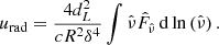
Initially, we attempted to fit the X-ray spectra of all sources using a simple power-law model, but this yielded poor fits, indicating the presence of intrinsic curvature in the spectra. Indeed, a log-parabola (logpar model in XSPEC) provides good statistical fits. The best-fit logpar model parameters along with their uncertainties estimated within a 90% confidence range are reported in Table 2, and the corresponding spectral fits are shown in Fig. 1. In all cases, the combined SXT and LAXPC spectra up to 10 keV are able to pin down the location of the synchrotron peaks well within the observed energy range. The peak energies (ϵp) are estimated using the eplogpar model included in XSPEC. For the first four sources (see Table 2), we observe hard spectral indices (α < 2) and synchrotron-peak energy values above 1 keV. For 1ES 0120+340 and 1ES 1741+196 in particular, the AstroSat observations provide the first well-constrained estimation of the synchrotron peak values. However, 1ES 2322–409 is an exception, satisfying the criteria of a regular HBL with a relatively soft spectral index and synchrotron peak located below 0.3 keV.
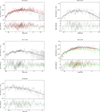 |
Fig. 1. Combined SXT and LAXPC-20 spectrum of 1ES 0120+340, RGB J0710+591 (A1: black; A2: red), 1ES 1101-232, 1ES 1741+196 (A1: black, A2: red; A3: green), and 1ES 2322-409(SXT only), (from left to right in top and bottom), fitted using the TBabs*logparabola model. |
Best-fit log-parabola model parameters of joint SXT–LAXPC spectrum using TBabs*logpar model.
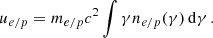
X-ray flux variability is seen in some of the sources over various timescales. For example, RGB J0710+591 shows a significant spectral transition with a strongly increasing spectral curvature (β increased by a factor ∼1.8) and a marginal change in its spectral index and flux over a period of one year (see Costamante et al. 2018; Goswami et al. 2020). The X-ray light curve in the energy range 0.3–7 keV obtained for the period February 2009–December 2017 (MJD 54882.18–58110.26) is shown in the bottom panel of Fig. 2. We first applied the Bayesian blocks algorithm (Scargle et al. 2013) implemented in astropy11 to the long light curve. We used the option of ‘measures’ in the fitness function and a false-alarm probability of p0 = 0.01. We observe long-term flux variations: high flux activity during February 2009–March 2009 (period P1) and February 2012–January 2013 (period P2), and low flux activity during January 2015–December 2017 (period P3). We further characterise the flux variations in these periods by their doubling/halving timescales (ΔtD/ΔtH), which are given as Δt = t × ln2/|ln(F2/F1)| (Saito et al. 2013). Here, F1 and F2 are the fluxes observed at a time interval of duration t. The highest flux is observed during period P1, with a flux of (8.6 ± 0.6)×10−11 erg cm−2 s−1. The flux during P2 shows a rise followed by a sharp decline and peaks at (7.8 ± 0.5)×10−11 erg cm−2 s−1 with ΔtD = 14.5 ± 2.68 days and ΔtH = 0.92 ± 0.11 days. The period P3 shows a slowly decaying trend with an estimated halving timescale of ΔtD = 29.7 ± 5.31 days. The overall variation can further be characterised by the fractional variability amplitude (following the definition by Vaughan et al. 2003). The mean fractional variability in the long-term light curve is ∼39.6%.
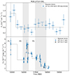 |
Fig. 2. Lightcurves of RGB J0710+591 overlaid with the Bayesian blocks representation. Top panel: Fermi-LAT in the energy range 0.3–300 GeV from 2008/09-2021/09 in 300-day bins in units of 10−9 cm−2 s−1. The upper limits correspond to 3σ limits. The dotted line represents the constant-fit. Bottom panel: Swift-XRT (in blue) and AstroSat-SXT (in black) in the energy range 0.3–7 keV in units of 10−11 erg cm−2 s−1. |
For 1ES 1741+196, we observe significant X-ray flux variations over a long observation period from 2010/07 to 2020/10. The mean fractional variability in the long-term light curve is ∼32.2%. To obtain significant spectra in the γ-ray band detected by Fermi-LAT, our sources require integration times of several years. For every source, we obtained spectra focused on the AstroSat observations (see Table 1). In the case of RGB J0710+591, 1ES 1101–232, and 1ES 1741+196, we also computed spectra that coincide with the archival VHE and X-ray (XRT/NuSTAR) observations used for the SED analysis. The Fermi-LAT integration times and spectral-fit parameters are provided in Table 3. The spectra are fitted with a power law in the energy range 0.3–300 GeV. The absorption effects due to EBL at these energies are likely negligible for the observed sources and therefore no corrections were made. The low photon indices (ΓLAT ≤ 1.6) of the observed spectra for 1ES 0120+340, RGB J0710+591, and 1ES 1101–232 indicate that the high-energy peak may be located at energies above 1 TeV, leading to their classification as extreme-TeV blazars. While the spectral indices in 1ES 1741+196 and 1ES 2322–409 are below 2.0, the soft VHE spectra (coupled with their X-ray spectra) result in their classification as an extreme-Syn blazar and an HBL, respectively. Overall, the individual Fermi-LAT spectra show consistent behaviour over extended periods of observations, except for RGB J0710+591. We find evidence of high flux activity in the extended light curve of this latter source (upper panel of Fig. 2), which coincides with the period P1. This is also illustrated by the presentation of Bayesian block generated with a p0 value of 0.01.
Best-fit power-law model parameters of observed Fermi-LAT spectrum.
4. Spectral modelling
In the previous section, we show that some sources are variable (RGB J0710+591 and 1ES 1741+196), while the others show seemingly constant flux. In order to properly model the SEDs of the five sources, we defined the data sets to be modelled (Sect. 4.1), and then derived constraints (Sect. 4.2). We then proceeded with modelling the data sets with four different setups (Sect. 4.3).
4.1. Data sets
We compiled data sets that are as complete and as contemporaneous as possible. The data sets are defined in Table 4 and the corresponding SEDs are shown in Fig. 3. As many bands are not covered simultaneously with any of the defined data sets, we also gathered additional non-contemporaneous data, which we label as archival data and show in grey in Fig. 3.
 |
Fig. 3. The MWL SEDs of 1ES 0120+340, RGB J0710+591, 1ES 1101–232, 1ES 1741+196, and 1ES 2322–409, respectively, with details given in the legends. The colored spectra follow the definition given in Table 4. |
Source power-law indices of the SED in the optical/UV-to-X-ray part, αox, and the HE γ-ray part, αγ, as well as the time ranges and collected data sets for the modelling.
In 1ES 0120+340, the two AstroSat spectra are compatible with each other, while they seem to be slightly softer than the earlier Swift-XRT spectrum. However, the LAXPC spectrum indicates that the cut-off is beyond 1017 Hz. We therefore consider only one spectrum for the modelling. Unfortunately, no VHE γ-ray data are publicly available, and therefore the high-energy peak of this extreme-TeV source is not well constrained.
RGB J0710+591 is a bona fide extreme-TeV source that is now firmly established as variable in both spectral components. We collect three MWL spectra for modelling: Spectrum 1 (black in Fig. 3), which is comprised of data from Swift, Fermi-LAT, and VERITAS; Spectrum 2 (blue in Fig. 3), containing data from Swift, NuSTAR, and Fermi-LAT; and Spectrum 3 (red in Fig. 3), with data from AstroSat and Fermi-LAT. In the X-ray domain, Spectrum 1 is both higher in flux and harder than Spectra 2 and 3. Additionally, from Spectrum 2 to 3, the peak frequency reduces. As the optical/UV fluxes seemingly do not change – possibly due to a significant contribution from the host (Acciari et al. 2010a) – the spectral index describing the spectrum from the UV to the X-ray domain drops from Spectrum 1 to Spectra 2 and 3. The Fermi-LAT spectra also indicate spectral variability with a softening throughout. The connection to the VHE γ-ray spectrum is not perfect for either of the Fermi-LAT spectra, suggesting that the VHE γ-ray spectrum is also variable.
In the extreme-TeV source 1ES 1101–232, the X-ray spectrum seems stable between the different observations from Swift + NuSTAR and AstroSat, although the maximum seems to be at a slightly lower energy in the AstroSat spectrum. However, the flux at the highest X-ray frequencies is unchanged compared to previous observations. Similarly, the HE γ-ray spectra are comparable and connect well with the VHE spectrum. Therefore, only one spectrum is considered in the modelling.
For 1ES 1741+196, we again collect three different spectra: Spectrum 1 (black in Fig. 3) comprised of data from Swift, Fermi-LAT, and MAGIC; Spectrum 2 (blue in Fig. 3) containing data from AstroSat (A1 + A2) and Fermi-LAT; and Spectrum 3 (red in Fig. 3) with data from AstroSat (A3) and the same Fermi-LAT spectrum as for Spectrum 2. There is noticeable flux and spectral variability in the X-ray domain, indicating a flux rise from Spectrum 1 to Spectrum 2. In the few months that pass between Spectrum 2 and Spectrum 3, the X-ray peak frequency drops. The optical/UV spectra seem to have a strong contribution from the host galaxy (hosted in a triplet of interacting galaxies; Ahnen et al. 2017) and the emission is roughly stable from Spectrum 1 to Spectrum 3. The spectral index from the optical/UV to the X-ray domain increases from Spectrum 1 to Spectrum 3. On the other hand, the γ-ray spectrum seems stable. Variations on monthly timescales, as in the X-ray domain, cannot be detected due to the low flux, which is also why only one spectrum is shown for periods 2 and 3. The overall soft γ-ray spectrum leads to the classification as an extreme-Syn source.
The HBL 1ES 2322–409 does not show significant spectral variation in the X-ray band. Compared to Swift observations, a mildly higher flux is noticeable. The HE and VHE γ-ray spectra are well connected despite the significant time span between the observations, also suggesting stable fluxes. Because of this stability, we only consider one spectrum for this source.
4.2. Constraints
The shape of the spectral components in the SEDs provides important constraints on the particle distributions. We define the spectral index α in a given energy range as νFν ∝ να. While the Fermi-LAT γ-ray spectrum directly gives us the γ-ray spectral index, αγ, we need to make an assumption on the shape of the synchrotron spectrum, as the X-ray spectra contain only peaks and cut-offs, but no broad power law, except for the HBL 1ES 2322–409. On the other hand, it is plausible that below the X-ray domain, the synchrotron spectrum resembles a power law smoothly connecting to lower energies. Unfortunately, in several cases, the UV data points are influenced by non-jetted emission (e.g. the host galaxy). While one can attempt a joint fit of the synchrotron power law and the galactic components (as in e.g. Wierzcholska & Wagner 2020), it is a reasonable approximation to ignore this influence. In turn, the spectral index derived from the UV to X-ray spectrum can be considered as a lower limit, that is, the synchrotron spectrum could be harder. The derived spectral indices of the optical/UV-to-X-ray range, αox, and the HE γ-ray range, αγ, are given in Table 4.
Within errors, αox and αγ agree for most sources and spectra. Given that 1ES 2322–409 is an HBL, the different values of αox and αγ are expected. It is nonetheless reassuring that for this source the index αox agrees well with the spectral index in the X-ray domain, suggesting that the synchrotron peak is located in the optical/UV range.
The synchrotron spectral index, αsy, is directly related to the spectral index of the injected or accelerated particle distribution, s, through the relation s = 3 − 2αsy for uncooled particles, and s = 2 − 2αsy for cooled particles. While the cooling status must be verified a posteriori, this can be used to constrain the electron spectral index from αox. Similarly, if the γ-rays stem from proton synchrotron emission, the proton distribution is directly given from αγ.
The lack of (observed) variability on timescales of shorter than a few days prevents us from obtaining any meaningful constraint on the source size. We therefore followed Cerruti et al. (2015), and employed standard one-zone sizes on the order of 1015 − 17 cm. These authors also revealed the existence of an inverse relation between source size and magnetic field strength while keeping the Lorentz factor of the cooling break constant, and showed that a relatively large range of the parameter space can produce reasonable fits. Furthermore, small region sizes and high magnetic fields result in a lower overall source power. We therefore concentrate on this parameter range.
The jet power is an important measure with which to quantify the plausibility of a model beyond a fit to the data. As the jet is anchored in the black hole–disk system, the jet power is tied to the power funnelled through the accretion disk to the black hole. The accretion power is therefore an important measure against which the jet power can be gauged. However, we have no direct observational evidence of the disk flux in any of our sources. In turn, we chose the accretion disk luminosities such that the summed flux of the disk and the jet does not overshoot the observed data. The obtained values are given in Table 5 and can be regarded as upper limits. We note that the employed radiation codes (see below) use standard Shakura-Sunyaev disks (Shakura & Sunyaev 1973), while HBL and eHBL sources are typically regarded as hosting radiatively inefficient accretion flows (RIAFs; e.g. Igumenshchev 2004). This implies that the obtained luminosity limits on the discs in Table 5 may not be the true accretion power, as RIAFs can sustain much higher accretion rates than suggested by their emitted radiation (Katz 1977; Czerny 2019; Ghodla & Eldridge 2023). Nonetheless, the luminosity limit may still provide important constraints.
Total jet powers  in erg s−1 for the various model fits, as well as the upper limit on the accretion disk power from the modelling.
Similarly, the masses of the supermassive black holes are uncertain or even unknown in our sources. In order to provide references in the discussions below, we provide the Eddington luminosity for a black hole with a mass of 1×10⁸(9) M⊙ being 1.3×1046(47) erg s−1. In any case, the inferred limits on the radiation output of the accretion discs are orders of magnitude below the Eddington limit.
The powers in the observer’s frame,  , for the radiation, the magnetic field, and the electron and proton populations are calculated with
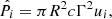 (1)
(1)
with the bulk Lorentz factor Γ and the energy density ui of the respective constituent. The energy density of the radiation, urad, is calculated from the model SED in the observer’s frame,  , with the relation (Zacharias & Wagner 2016)
 (2)
(2)
The magnetic energy density is uB = B2/8π, while the particle energy densities are given as
 (3)
(3)
There are two caveats here. First, in the SSC model, we assume one cold proton per electron, giving the proton energy density as up = mpc2∫ne(γ) dγ . Second, the proton power in the other models depends strongly on the minimum proton Lorentz factor, γmin, p, which we assume to be close to unity owing to the lack of constraints. Larger values of γmin, p could reduce the proton power substantially. The total jet power,  , is the sum of the four constituents and is listed for each source and model in Table 5. The individual powers are given in Appendix B.
4.3. Modelling
We use various codes to model the SEDs of our sources. Here, we only describe the purpose of the codes and the results, while brief code descriptions including definitions of the free parameters are provided in Appendix A. In all cases, the model curves were derived as fits by eye, as a broad range of solutions is possible in all cases (e.g. Cerruti et al. 2015). Steady-state solutions were obtained for all SEDs given the lack of variability information on short timescales as well as the non-simultaneity of the data.
Firstly, we derived a simple leptonic one-zone SSC model (hereafter referred to as SSC) using the steady-state code of Böttcher et al. (2013). In the plots of the SED fits, this model is shown as the red solid line. Secondly, we used the electron–proton co-acceleration model (hereafter referred to as e-p-shock) of Zech & Lemoine (2021). The advantage of this model is a physical motivation of the hard electron distribution. However, as this model is specifically designed to explain hard intrinsic VHE spectra, it was only applied to the extreme-TeV sources 1ES 0120+340, RGB J0710+591, and 1ES 1101–232. A magenta dash-double-dotted line marks this model in the SED-fit plots. Thirdly, we employed the lepto-hadronic code ONEHALE (version 1.1, Zacharias 2021; Zacharias et al. 2022). We produced two solutions with this code. The first one is a lepto-hadronic model (hereafter referred to as LHπ), where the γ-rays are produced from electron-synchrotron emission by secondary pairs (from Bethe-Heitler pair production, photo-pion production, and γγ pair production). Here, we chose to suppress the SSC contribution, which can be prominent in an LHπ model (cf., Cerruti et al. 2015). Blue dashed lines show this model. The second solution is a proton-synchrotron model (hereafter referred to as LHp) designed to describe the γ-rays, which is displayed as orange dash-dotted lines.
Below, we discuss each source in turn, providing individual SED fits. The complete sets of model parameters are given in Appendix B. Given the large number of free parameters, especially in the lepto-hadronic models, we tried to keep as many parameters as possible fixed from model to model as well as from source to source. This includes the Doppler factor, δ, the escape and acceleration time parameters, ηesc and ηacc, and, in the lepto-hadronic models, the magnetic field B.
For instance, we fix the Doppler factor to δ = 50 in all cases and also employ δ = Γ. While this is a large value, and sometimes better fits are possible with lower values, it removes an ambiguity between the models and eases the interpretation. In turn, the main differences in the modelling are related to the particle distributions and the size of the emission region.
4.3.1. 1ES 0120+340
The fits to 1ES 0120+340 are shown in Fig. 4, while the model parameters are given in Table B.1. The fits to the data are generally good. Differences occur in the VHE γ-ray domain, which could become an important discriminator should this source be established as a VHE source in future observations. Modelling 1ES 0120+340 with the e-p-shock model assuming acceleration on a single shock did not yield a satisfactory result. Allowing reacceleration on a second shock provides us with a good fit. The LHπ model results in a flat spectrum above 1020 Hz. The model MeV bump is synchrotron emission from Bethe-Heitler-pair-produced electrons, while the GeV bump is synchrotron emission of electrons from γ–γ pair production and pion production. No VHE γ-ray emission is expected from this model.
 |
Fig. 4. Main (red) and archival (grey) data sets of 1ES 0120+340, as well as the various intrinsic models: SSC (red solid line), e-p-shock (magenta dash-double-dotted line), LHπ (blue dashed line), and LHp (orange dot-dashed line). The thin grey line marks the host galaxy template of Silva et al. (1998). |
The particle spectral indices in the SSC and LHπ models suggest that the particles are cooled. In the LHp case, this is only true for the electrons, while the protons are not cooled. This requires a softer proton injection distribution compared to the electrons. We point out here that in the e-p-shock model the hardening of the electron distribution after injection due to (additional) acceleration is taken into account. Therefore, the consideration concerning the injection spectral index of the particle distributions derived from the observed spectra does not apply.
The other parameters are comparable with the other sources below with no significant outlier. However, it is interesting that the optical–X-ray and HE γ-ray spectra are among the hardest ones in our list of sources, requiring very hard particle injection distributions.
In all models, the jet power is particle-dominated. All total jet powers exceed the accretion disk luminosity limit derived from the modelling. While the SSC model and the e-p-shock model are within an order of magnitude of the disc limit, the LHπ and LHp models exceed the limit by several orders of magnitude. The LHπ model even exceeds the Eddington luminosity of a 109 M⊙ black hole.
4.3.2. RGB J0710+591
There are significant differences between the three SEDs shown in Fig. 5. Spectrum 1 exhibits the highest X-ray flux, as well as the hardest HE γ-ray spectrum. Indeed, judging from Fig. 2, RGB J0710+591 was in a prolonged HE high-state during this time with a subsequent flux decrease. This decrease is accompanied by a softening of the HE spectrum. Unfortunately, no data exist for the VHE γ-ray spectrum for the later epochs, but a flux drop is likely along with the softening of the HE spectrum; although, we must note that the VHE spectrum might still be consistent with an extension of the later HE spectra within statistical errors. The X-ray spectrum drops in flux and seemingly exhibits spectral changes in the later data sets. While the first X-ray spectrum is compatible with a pure power law with αX = 0.25, the second spectrum clearly indicates a curved spectrum with a peak below 10 keV, which further drops in Spectrum 3. However, we cannot rule out the presence of such a peak in Spectrum 1 given the limited spectral coverage of Swift-XRT. Interestingly, the optical–X-ray spectra in the second and third data sets are much softer than the first one, suggesting that the underlying electron distribution has softened. The parameter sets for the three spectra are given in Tables B.2–B.4, respectively.
 |
Fig. 5. Main (color) and archival (grey) data sets of RGB J0710+591, as well as the various intrinsic models (Top: for Spectrum 1 (black); Middle: for Spectrum 2 (blue); Bottom: for Spectrum 3 (red)): SSC (red solid line), e-p-shock (magenta dash-double-dotted line), LHπ (blue dashed line), and LHp (orange dot-dashed line). VHE γ-ray data have been corrected for EBL absorption. The thin grey line marks the host galaxy template of Silva et al. (1998). |
With the exception of the LHπ model, the fits are good for the various models in all three states. The poor LHπ model fit is due to the imposed constraint that ensures consistency with the upper limits at the lowest γ-ray energies, which makes it impossible to reproduce the subsequent hard γ-ray spectrum up to the VHE domain.
In the SSC model and the LHπ model, the particle distributions are cooled, while this is only true for the electrons in the LHp model. In the latter, the protons are uncooled, leading to a softer injection distribution compared to the electrons. This is true for all three source states.
In order to accommodate the changes between the data sets, relatively minor changes must be made from one data set to another. In the SSC model, the main change is in the magnetic field, which drops from 0.03 G to 0.02 G and 0.015 G. An increase in the electron power is required from Spectrum 1 to Spectrum 2 in order to account for the slightly rising peak-flux ratio between the low- and the high-energy components of the SED. The power drops then to Spectrum 3, and the maximum electron Lorentz factor is reduced.
Generally, the parameters are consistent with the modelling of Acciari et al. (2010a) and Costamante et al. (2018). The parameters of Katarzyński (2012) differ from our estimates as this author used a much lower Doppler factor of δ = 8. In the e-p-shock model, we find a continuous increase in the radius and a continuous decrease in the magnetic field from one spectrum to the next. However, the electron distribution does not change from Spectrum 1 to Spectrum 2, and only reduces mildly in energy density to Spectrum 3. The energy density of the proton distribution (which is important for the electron acceleration) drops continuously from Spectrum 1 to Spectrum 3. This behaviour is reminiscent of adiabatic expansion of the emission region (Boula & Mastichiadis 2022; Zacharias 2023), but the magnetic field strength varies too rapidly with respect to the radius and the overall timescale is much too long to be explained with the relativistic movement of a blob along the jet.
As we keep the magnetic field constant in the LHπ model, the spectral changes are mostly accounted for through a reduction in the electron injection power, as well as shifts in the minimum and maximum electron Lorentz factors. In order to produce the secondary electron population, the proton distribution has to be changed in a non-trivial manner. In order to accommodate the reduced upper limits in Spectrum 2 compared to Spectrum 1, the maximum proton Lorentz factor must be reduced to shift the cut-off in the Bethe-Heitler component (the peak at ∼1021 Hz) to lower energies. However, this requires an increase in the proton power to achieve the flux of the upper limits. The proton power is reduced again in order to account for Spectrum 3.
In comparison to the modelling in Cerruti et al. (2015), we employed a smaller emission region and a higher magnetic field to suppress the SSC contribution, a method also employed in Cerruti et al. (2015). This choice also has consequences for the proton distribution; these latter authors use a higher maximum proton Lorentz factor and a lower proton power than in our modelling. The LHp model requires more important adjustments from one case to another because of the change in the HE γ-ray domain. The softening of the HE spectrum is best reproduced by a softening of the proton distribution plus an increase in the magnetic field. The latter shifts the synchrotron spectrum to higher energies, allowing an improved representation of the γ-ray data. In addition, the proton power must be increased considerably to counter the flux reduction at the highest energies due to the softening of the proton distribution. The increase in the magnetic field requires a significant reduction in the minimum and maximum electron Lorentz factors from Spectrum 1 to Spectrum 2 along with the drop in particle power. The parameter sets are generally in the range obtained by Cerruti et al. (2015).
In all our cases, the jet power is particle dominated and exceeds the inferred upper limit of the accretion disc. Interestingly, for all models, the jet power does not decrease from one state to another, as one would expect from the observed flux drops (see Table 5). The SSC model barely requires any change in jet power, while in the e-p-shock model, the power even increases as the decrease in magnetic field strength is countered by an increase in the particle power. In the LHπ model, Spectrum 2 exhibits the highest jet power due to the required increase in proton power. In all three states, the jet power in the LHπ model surpasses the Eddington power of a 109 M⊙ black hole. The aforementioned increase in the proton power in the LHp model induces an increase in jet power similar to the e-p-shock model. For Spectrum 1, the LHp jet power is below the Eddington luminosity of a 108 M⊙ black hole, while it surpasses that of a 109 M⊙ black hole in Spectrum 312.
4.3.3. 1ES 1101–232
The fits for this source are displayed in Fig. 6, while the parameters can be found in Table B.5. The e-p-shock model and the LHp model reproduce the data well, while the SSC model and the LHπ model cannot reproduce the (archival) VHE data. Additionally, the LHπ model does not work well for the low-energy part of the HE γ-ray spectrum.
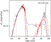 |
Fig. 6. Main (red) and archival (grey) data sets of 1ES 1101−232, as well as the various intrinsic models: SSC (red solid line), e-p-shock (magenta dash-double-dotted line), LHπ (blue dashed line), and LHp (orange dot-dashed line). VHE γ-ray data have been corrected for EBL absorption. The thin grey line marks the host galaxy template of Silva et al. (1998). |
The particle distributions in the SSC model and the LHπ model are cooled, which also holds for the electrons in the LHp model. However, the protons in the LHp model are uncooled, resulting in a softer injection distribution than the electrons.
The jet power is particle dominated in all cases, and all models surpass the inferred upper limit of the accretion disk luminosity. The LHπ model exceeds the Eddington power of a 109 M⊙ black hole, while the LHp model requires at least a black hole of mass 7×10⁸ M⊙ in order to remain sub-Eddington.
This source has also been modelled by other authors. Aharonian et al. (2007b) and Costamante et al. (2018) employed SSC models. Given the difference in the Doppler factors used between each other and with respect to our modelling, the difference in the other parameters is obvious. The e-p-shock model was already considered for this source in Zech & Lemoine (2021). Compared to their work, we require a larger emission region and smaller particle density and magnetic field strength given a slightly different spectral shape in the X-ray domain. Particle acceleration must occur at two shocks in order to achieve a reasonable fit.
Cerruti et al. (2015) produced lepto-hadronic models for this source13. While their LHπ model fits the VHE data, it also suggests a significant Bethe-Heitler component, which would overwhelm our HE γ-ray spectrum even more than our LHπ model already does. This suggests that this model is indeed not a good solution for this source. Their LHp model parameters are very similar to ours.
4.3.4. 1ES 1741+196
Due to its flat HE γ-ray spectrum, we categorise 1ES 1741+196 as an extreme-Syn source. As the e-p-shock model has been set up specifically to describe the very narrow spectral bumps of extreme TeV blazars, it is not applicable to this source in its current form. Nonetheless, the source shows an interesting MWL evolution from state to state. Spectrum 1 indicates a soft optical/UV–X-ray spectrum with αox ∼ 0.1, implying a soft underlying electron distribution with se ∼ 1.8. Surprisingly, the hardening of the synchrotron spectra between the two AstroSat observations is not reflected in the HE γ-ray spectrum. This complicates the interpretation. The models are shown in Fig. 7, while the parameters are listed in Tables B.6–B.8.
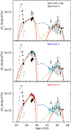 |
Fig. 7. Main (colour) and archival (grey) data sets of 1ES 1741+196, as well as the various intrinsic models (Top: For Spectrum 1 (black). Middle: For Spectrum 2 (blue). Bottom: For Spectrum 3 (red)): SSC (red solid line), LHπ (blue dashed line), and LHp (orange dot-dashed line). VHE γ-ray data have been corrected for EBL absorption. The thin grey line marks the host galaxy template of Silva et al. (1998). |
The three applied models reproduce all three data sets fairly well. In the SSC model and the LHπ model, the particle distributions are cooled. In the LHp model, the proton distribution is uncooled, while the electron distribution is cooled. In turn, the proton injection distribution is softer than the electron distribution.
As mentioned above, the X-ray spectrum shows significant variability, while the γ-ray spectrum remains steady. From Spectrum 1 to Spectrum 2, the X-ray flux rises by at least a factor 3 with a mild subsequent drop to Spectrum 3. The X-ray peak frequency does not seem to shift significantly from state to state, although a clear determination of the peak in Spectrum 1 is not possible. In order to reproduce these changes with the SSC model, the most important change is a higher particle power in addition to a change in the particle spectral index. The radius and the magnetic field change by 50% at most. The escape time factor, ηesc = 400, is very high. An SSC model was also employed by Abeysekara et al. (2016) and Ahnen et al. (2017). However, their X-ray spectra do not show the cut-off that we see, especially with the AstroSat data. Therefore, our electron energy distribution is much more restricted. As we use a higher Doppler factor than either of those earlier works, the differences in radius (ours being smaller) and magnetic field (ours being higher) are reasonable. In the LHπ model and the LHp model, the variations in our spectra can be reconciled easily, with minor changes of at most a factor 2 in the parameters.
In all our cases, the total jet power is dominated by particles and surpasses the inferred upper limit of the accretion disc luminosity. Both the LHπ model and the LHp model exceed the Eddington luminosity of a 109 M⊙ black hole in all three data sets owing to the soft proton distribution requiring a large power.
4.3.5. 1ES 2322–409
This is a classical HBL source with a soft X-ray spectrum. The e-p-shock model is therefore not applied here either. The fits are displayed in Fig. 8, while the parameters are given in Table B.9.
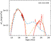 |
Fig. 8. Main (red) and archival (grey) data sets of 1ES 2322−409, as well as the various intrinsic models: SSC (red solid line), LHπ (blue dashed line), and LHp (orange dot-dashed line). VHE γ-ray data have been corrected for EBL absorption. |
The SSC model and the LHp model fit the data very well, while we were not able to find an acceptable fit for the LHπ model. The reason is the low synchrotron peak energy and, in turn, the soft X-ray spectrum. As these are the target photons for the pγ interactions, even a very hard proton distribution would not produce a significant secondary flux from pion decay, which is needed in the HE domain. Additionally, due to the soft X-ray target photon field, γγ pair production also contributes very little to the HE domain. These two effects diminish the synchrotron peak at HE γ-rays, which is produced by secondary electrons from these two interaction channels.
The electron distributions in all models are cooled, while the proton distributions in the LHπ and LHp models are uncooled. Nonetheless, for this source, this implies that the spectral indices of the electron and proton injection distributions are equal in the lepto-hadronic models.
The remaining parameters are well in line with parameters for other HBL sources. This is best exemplified by the fact that the parameters of our SSC model agree very well with the parameter set of Abdalla et al. (2019).
The total jet power is particle dominated in all cases. While the SSC model only barely exceeds the inferred upper limit of the accretion disk luminosity, the LHπ model and the LHp model exceed this limit by orders of magnitude and even exceed the Eddington luminosity of a 109 M⊙ black hole.
Even though this source shows peak frequencies that are more commonly seen in regular HBLs, the low value of the magnetic field strength and high value of the minimum electron Lorentz factor required for the SSC model indicate some common features with extreme TeV blazars.
5. Discussion and conclusions
In this paper, we present an analysis of data for three extreme-TeV sources, one extreme-Syn, and one HBL source observed with AstroSat and other instruments. For the first time, we establish the X-ray peak energy in two sources, namely 1ES 0120+340 and 1ES 1741+196. The former source exhibits extreme-TeV characteristics and is therefore a VHE-γ-ray-detection candidate. A VHE γ-ray detection would strongly constrain the model parameter space. Furthermore, while 1ES 0120+340 and 1ES 1102–232 do not show any variability compared to archival data sets, clear variability is established in RGB J0710+591 and 1ES 1741+196. The HBL 1ES 2322–409 does not show variability in our data sets; however, it is known to be variable at least in the synchrotron component (Abdalla et al. 2019).
RGB J0710+591 exhibits both flux and spectral variability in the X-ray and γ-ray bands. The X-ray long-term light curve (Fig. 2) shows variations on timescales of days to weeks, while a marginally significant high state in the γ-ray band is visible in the first years of observations. The long-lasting downward trend in the X-ray light curve over the following few years of observations is accompanied by a drop in the X-ray peak frequency (Fig. 3). On similar timescales, the γ-ray spectrum softens. Given that neither of the Fermi-LAT spectra connects well to the archival TeV spectrum, the latter energy range might also be variable. Additional observations in that domain should clarify this point. The reproduction of the changes requires non-trivial parameter changes depending on the chosen model, as described in Sect. 4.3.2. While none of the solutions are unique, and different parameter sets might provide equivalent fits, these results suggest that there is no simple physical explanation for these changes.
On the contrary, 1ES 1741+196 shows variability mainly in the X-ray domain, while there is no obvious variability in the optical and γ-ray regimes. The changes in X-ray spectra imply that the electron distribution has to change from one spectrum to the next in order to accommodate the relative change between the optical and X-ray fluxes. This actually makes it complicated to account for the non-changing γ-ray spectrum in a leptonic model, which is reflected in the way the parameters have to be changed. This is the advantage of the LHπ and LHp models, as the proton distribution does not need to be changed. However, the power demand of the lepto-hadronic models is a problem.
Indeed, the modelling results highlight the advantages and disadvantages of the various models. The SSC model is clearly the most conservative in terms of power requirements, but it has some issues with reproducing the full γ-ray spectra in the eHBL sources. The LHp model has no difficulty in reproducing spectra owing to its large number of free parameters, but it has a huge power demand. Similarly, the LHπ model requires a large amount of power and additionally has problems properly reproducing the γ-ray spectra. This is related to the fact that we specifically suppressed the SSC contribution in the LHπ model resulting in an almost flat synchrotron SED of the secondary electrons. Fits with the LHπ model improve when allowing an SSC contribution (e.g. Cerruti et al. 2015). However, this does not reduce the power demand. All three models suffer from the fact that they are not designed to self-consistently explain the very hard particle injection distributions. The LHp model has an additional complication in that the proton and electron injection distributions do not exhibit the same power-law index. However, one would expect the injection distributions from electrons and protons to achieve more or less the same spectral index if they were accelerated at the same shock or through the same process.
This is the benefit of the e-p-shock model, which naturally explains the hard electron distributions as being due to electron–proton co-acceleration at (multiple) shocks. However, by design, this model only works in extreme-TeV sources with a hard intrinsic VHE spectrum. In sources with a softer VHE spectrum (like extreme-Syn sources and classical HBLs), the model is not directly applicable. Additionally in this scenario, one has to assume a large increase of between 102 and 103 in the magnetisation between the upstream and downstream regions in extreme-TeV sources, while the upstream magnetisation is rather low (of the order of 10−6). As pointed out by Tavecchio et al. (2022), such a low magnetisation may be a problem when ascribing the shocks to recollimation, given that 3D MHD simulations indicate that only a single recollimation shock appears for sufficiently low magnetisation because of instabilities that induce turbulence in the jet downstream of the recollimation shock. However, the amplification of the magnetisation in the downstream region due to the particle stream might have an impact on the growth of turbulence. Other factors might also play a role, such as jet stratification or the structure of large-scale magnetic fields.
As is typically observed for extreme blazars, all the objects in our sample require low magnetic fields (order of 10 mG, except for 1ES 1741+196) and high minimum electron Lorentz factors (> 103) in the SSC and e-p-shock models. The HBL 1ES 2322-409 shares these characteristics with the bona fide extreme blazars.
The jet power in all our models (including SSC and e-p-shock) is above the inferred upper limits of the accretion disk luminosities. While in the SSC model this may be due to parameter choices, such a result is in line with the conclusion of Ghisellini et al. (2014), who found this to be a general feature in (high-power) blazars by comparing the observed γ-ray luminosity with inferred accretion disk luminosities.
As mentioned above, HBLs and eHBLs are probably powered by RIAFs, suggesting that the inferred radiation limits underpredict the true accretion power. Nevertheless, it is remarkable that the inferred limits on the disks are on the order of one millionth of the Eddington luminosity of even a 108 M⊙ black hole.
In summary, the AstroSat and MWL observations show that extreme blazars exhibit various characteristics. While some of them are stable, others are variable on timescales of years, as well as on shorter timescales. Also, while RGB J0710+591 varies in both X-rays and γ-rays, 1ES 1741+196 only varies in the X-ray domain. The modelling suggests a preference for leptonic models, because of the power demand; although all of our models exceed the obtained upper limits of the accretion disk luminosity, which is a curious fact. Given that lepto-hadronic models seem unlikely, we do not expect neutrinos to be emitted by these sources. In addition, neutrino production requires photon fields of much greater intensity than those present in these sources (Reimer et al. 2019).
A study like ours would significantly benefit from long-term VHE γ-ray observations by Cherenkov telescopes. Unfortunately, no such data exist at the moment. As VHE γ-rays probe the high-energy peak of extreme blazars, they provide clues that are vital to modelling these sources, as well as valuable insights into their characteristics and especially their variability. Proper MWL campaigns lasting several years will be crucial in order to gain more rigorous insights, which will not only be useful for studies of the sources themselves, but also for related studies, such as those probing the intergalactic magnetic field (Aharonian et al. 2023).
http://astrosat-ssc.iucaa.in/?q=sxtData
https://irsa.ipac.caltech.edu/applications/DUST/
https://fermi.gsfc.nasa.gov/cgi-bin/ssc/LAT/LATDataQuery.cgi
https://www.swift.ac.uk/analysis/uvot/
https://www.swift.ac.uk/analysis/xrt/
https://heasarc.gsfc.nasa.gov/docs/nustar/analysis/
https://heasarc.gsfc.nasa.gov/cgi-bin/Tools/w3nh/w3nh.pl
https://docs.astropy.org/en/stable/api/astropy.stats.bayesian_blocks.html
We made the generic comparisons for consistency with the other sources. However, RGB J0710+591 is the only source in our sample with a mass estimate of the black hole: log MBH = 8.25 ± 0.22 (Woo et al. 2005). The corresponding Eddington luminosity is LEdd = 2.34×1046 erg s−1.
Their HE γ-ray spectrum is rather soft, as the spectrum from the 2FGL catalogue was used, which has very limited statistics.
Acknowledgments
The OneHaLe code is available upon reasonable request to M. Z. This research has used the data of AstroSat mission of the Indian Space Research Organization (ISRO), archived at the Indian Space Science Data Centre (ISSDC). This work has used the data from the Soft X-ray Telescope (SXT) developed at TIFR, Mumbai, and the SXT POC at TIFR is thanked for verifying and releasing the data via the ISSDC data archive and providing the necessary software tools. We acknowledge the High Energy Astrophysics Science Archive Research Center (HEASARC), which is a service of the Astrophysics Science Division at NASA/GSFC for providing data and/or software. This research has made use of the XRT Data Analysis Software (XRTDAS) developed by the ASI Space Science Data Center (SSDC, Italy) and NuSTAR Data Analysis Software (NuSTARDAS) jointly SSDC, Italy and the California Institute of Technology (Caltech, USA). The Fermi Science Support Center (FSSC) team is acknowledged for providing the data and analysis tools. M. Z. acknowledges funding by the Deutsche Forschungsgemeinschaft (DFG, German Research Foundation) – project number 460248186 (PUNCH4NFDI). I. S. acknowledges support by the National Research Foundation of South Africa (Grant Number 132276).
References
- Abdalla, H., Aharonian, F., Ait Benkhali, F., et al. 2019, MNRAS, 482, 3011 [Google Scholar]
- Abdo, A. A., Ackermann, M., Agudo, I., et al. 2010, ApJ, 716, 30 [NASA ADS] [CrossRef] [Google Scholar]
- Abdollahi, S., Acero, F., Ackermann, M., et al. 2020, ApJS, 247, 33 [Google Scholar]
- Abeysekara, A. U., Archambault, S., Archer, A., et al. 2016, MNRAS, 459, 2550 [NASA ADS] [CrossRef] [Google Scholar]
- Acciari, V. A., Aliu, E., Arlen, T., et al. 2010a, ApJ, 715, L49 [NASA ADS] [CrossRef] [Google Scholar]
- Acciari, V. A., Aliu, E., Beilicke, M., et al. 2010b, ApJ, 709, L163 [NASA ADS] [CrossRef] [Google Scholar]
- Acciari, V. A., Ansoldi, S., Antonelli, L. A., et al. 2020, ApJS, 247, 16 [Google Scholar]
- Aguilar-Ruiz, E., Fraija, N., Galván-Gámez, A., & Benítez, E. 2022, MNRAS, 512, 1557 [NASA ADS] [CrossRef] [Google Scholar]
- Aharonian, F., Akhperjanian, A. G., Barres de Almeida, U., et al. 2007a, A&A, 475, L9 [CrossRef] [EDP Sciences] [Google Scholar]
- Aharonian, F., Akhperjanian, A. G., Bazer-Bachi, A. R., et al. 2007b, A&A, 470, 475 [NASA ADS] [CrossRef] [EDP Sciences] [Google Scholar]
- Aharonian, F. A., Khangulyan, D., & Costamante, L. 2008, MNRAS, 387, 1206 [NASA ADS] [CrossRef] [Google Scholar]
- Aharonian, F., Aschersleben, J., Backes, M., et al. 2023, ApJ, 950, L16 [NASA ADS] [CrossRef] [Google Scholar]
- Ahnen, M. L., Ansoldi, S., Antonelli, L. A., et al. 2017, MNRAS, 468, 1534 [NASA ADS] [CrossRef] [Google Scholar]
- Aliu, E., Archambault, S., Arlen, T., et al. 2014, ApJ, 782, 13 [NASA ADS] [CrossRef] [Google Scholar]
- Antia, H. M., Yadav, J. S., Agrawal, P. C., et al. 2017, ApJS, 231, 10 [NASA ADS] [CrossRef] [Google Scholar]
- Arnaud, K. A. 1996, ASP Conf. Ser., 101, 17 [Google Scholar]
- Biteau, J., Prandini, E., Costamante, L., et al. 2020, Nat. Astron., 4, 124 [Google Scholar]
- Blandford, R. D., & Rees, M. J. 1978, Phys. Scr., 17, 265 [CrossRef] [Google Scholar]
- Bloom, S. D., & Marscher, A. P. 1996, ApJ, 461, 657 [NASA ADS] [CrossRef] [Google Scholar]
- Bonnoli, G., Tavecchio, F., Ghisellini, G., & Sbarrato, T. 2015, MNRAS, 451, 611 [NASA ADS] [CrossRef] [Google Scholar]
- Böttcher, M., Dermer, C. D., & Finke, J. D. 2008, ApJ, 679, L9 [CrossRef] [Google Scholar]
- Böttcher, M., Reimer, A., Sweeney, K., & Prakash, A. 2013, ApJ, 768, 54 [Google Scholar]
- Boula, S., & Mastichiadis, A. 2022, A&A, 657, A20 [NASA ADS] [CrossRef] [EDP Sciences] [Google Scholar]
- Cerruti, M., Zech, A., Boisson, C., & Inoue, S. 2015, MNRAS, 448, 910 [Google Scholar]
- Costamante, L., Ghisellini, G., Giommi, P., et al. 2001, A&A, 371, 512 [NASA ADS] [CrossRef] [EDP Sciences] [Google Scholar]
- Costamante, L., Bonnoli, G., Tavecchio, F., et al. 2018, MNRAS, 477, 4257 [NASA ADS] [CrossRef] [Google Scholar]
- Czerny, B. 2019, Universe, 5, 131 [NASA ADS] [CrossRef] [Google Scholar]
- Dermer, C. D., Schlickeiser, R., & Mastichiadis, A. 1992, A&A, 256, L27 [NASA ADS] [Google Scholar]
- Fitzpatrick, E. L. 1999, PASP, 111, 63 [Google Scholar]
- Foffano, L., Prandini, E., Franceschini, A., & Paiano, S. 2019, MNRAS, 486, 1741 [NASA ADS] [CrossRef] [Google Scholar]
- Ghisellini, G., & Maraschi, L. 1989, ApJ, 340, 181 [NASA ADS] [CrossRef] [Google Scholar]
- Ghisellini, G., Tavecchio, F., Maraschi, L., Celotti, A., & Sbarrato, T. 2014, Nature, 515, 376 [NASA ADS] [CrossRef] [Google Scholar]
- Ghodla, S., & Eldridge, J. J. 2023, MNRAS, 523, 1711 [NASA ADS] [CrossRef] [Google Scholar]
- Goswami, P., Sinha, A., Chandra, S., et al. 2020, MNRAS, 492, 796 [NASA ADS] [CrossRef] [Google Scholar]
- Igumenshchev, I. V. 2004, Prog. Theor. Phys. Suppl., 155, 87 [CrossRef] [Google Scholar]
- Kalberla, P. M. W., Burton, W. B., Hartmann, D., et al. 2005, A&A, 440, 775 [NASA ADS] [CrossRef] [EDP Sciences] [Google Scholar]
- Katarzyński, K. 2012, A&A, 537, A47 [NASA ADS] [CrossRef] [EDP Sciences] [Google Scholar]
- Katarzyński, K., Ghisellini, G., Tavecchio, F., Gracia, J., & Maraschi, L. 2006, MNRAS, 368, L52 [Google Scholar]
- Katz, J. I. 1977, ApJ, 215, 265 [NASA ADS] [CrossRef] [Google Scholar]
- Kaufmann, S., Wagner, S. J., Tibolla, O., & Hauser, M. 2011, A&A, 534, A130 [NASA ADS] [CrossRef] [EDP Sciences] [Google Scholar]
- Kumar, A., Ghosh, S. K., Hutchings, J., et al. 2012, SPIE, 8443, 84431N [NASA ADS] [Google Scholar]
- Lefa, E., Rieger, F. M., & Aharonian, F. 2011, ApJ, 740, 64 [NASA ADS] [CrossRef] [Google Scholar]
- Li, W.-J., Xue, R., Long, G.-B., et al. 2022, A&A, 659, A184 [NASA ADS] [CrossRef] [EDP Sciences] [Google Scholar]
- Mannheim, K., & Biermann, P. L. 1992, A&A, 253, L21 [NASA ADS] [Google Scholar]
- Mücke, A., & Protheroe, R. J. 2001, Astropart. Phys., 15, 121 [Google Scholar]
- Reimer, A., Böttcher, M., & Buson, S. 2019, ApJ, 881, 46 [Google Scholar]
- Saito, S., Stawarz, Ł., Tanaka, Y. T., et al. 2013, ApJ, 766, L11 [Google Scholar]
- Scargle, J. D., Norris, J. P., Jackson, B., & Chiang, J. 2013, ApJ, 764, 167 [Google Scholar]
- Shakura, N. I., & Sunyaev, R. A. 1973, A&A, 24, 337 [NASA ADS] [Google Scholar]
- Sikora, M., Begelman, M. C., & Rees, M. J. 1994, ApJ, 421, 153 [Google Scholar]
- Silva, L., Granato, G. L., Bressan, A., & Danese, L. 1998, ApJ, 509, 103 [Google Scholar]
- Singh, K. P., Tandon, S. N., Agrawal, P. C., et al. 2014, SPIE Conf. Ser., 9144, 91441S [Google Scholar]
- Singh, K. P., Stewart, G. C., Chandra, S., et al. 2016, SPIE Conf. Ser., 9905, 99051E [NASA ADS] [Google Scholar]
- Singh, K. P., Stewart, G. C., Westergaard, N. J., et al. 2017, J. Astrophys. Astron., 38, 29 [NASA ADS] [CrossRef] [Google Scholar]
- Tandon, S. N., Subramaniam, A., Girish, V., et al. 2017, AJ, 154, 128 [NASA ADS] [CrossRef] [Google Scholar]
- Tavecchio, F., Ghisellini, G., Foschini, L., et al. 2010, MNRAS, 406, L70 [NASA ADS] [Google Scholar]
- Tavecchio, F., Costa, A., & Sciaccaluga, A. 2022, MNRAS, 517, L16 [NASA ADS] [CrossRef] [Google Scholar]
- Urry, C. M., & Padovani, P. 1995, PASP, 107, 803 [NASA ADS] [CrossRef] [Google Scholar]
- Vaughan, S., Edelson, R., Warwick, R. S., & Uttley, P. 2003, MNRAS, 345, 1271 [Google Scholar]
- Wierzcholska, A., & Wagner, S. J. 2020, MNRAS, 496, 1295 [NASA ADS] [CrossRef] [Google Scholar]
- Wolter, A., Tavecchio, F., Caccianiga, A., Ghisellini, G., & Tagliaferri, G. 2000, A&A, 357, 429 [NASA ADS] [Google Scholar]
- Woo, J.-H., Urry, C. M., van der Marel, R. P., Lira, P., & Maza, J. 2005, ApJ, 631, 762 [Google Scholar]
- Wood, M., Caputo, R., Charles, E., et al. 2017, Int. Cosmic Ray Conf., 301, 824 [Google Scholar]
- Yadav, J. S., Agrawal, P. C., Antia, H. M., et al. 2016, SPIE Conf. Ser., 9905, 99051D [NASA ADS] [Google Scholar]
- Yan, D., Zeng, H., & Zhang, L. 2012, MNRAS, 424, 2173 [NASA ADS] [CrossRef] [Google Scholar]
- Zacharias, M. 2021, Physics, 3, 1098 [NASA ADS] [CrossRef] [Google Scholar]
- Zacharias, M. 2023, A&A, 669, A151 [NASA ADS] [CrossRef] [EDP Sciences] [Google Scholar]
- Zacharias, M., & Wagner, S. J. 2016, A&A, 588, A110 [NASA ADS] [CrossRef] [EDP Sciences] [Google Scholar]
- Zacharias, M., Reimer, A., Boisson, C., & Zech, A. 2022, MNRAS, 512, 3948 [NASA ADS] [CrossRef] [Google Scholar]
- Zacharopoulou, O., Khangulyan, D., Aharonian, F. A., & Costamante, L. 2011, ApJ, 738, 157 [NASA ADS] [CrossRef] [Google Scholar]
- Zech, A., & Lemoine, M. 2021, A&A, 654, A96 [NASA ADS] [CrossRef] [EDP Sciences] [Google Scholar]
Appendix A: Code description
In this section, we provide brief overviews of the codes used for the modelling of our sources.
A.1. Steady-state leptonic one-zone model
The code was developed by Böttcher et al. (2013), and calculates the radiative output of an electron distribution ne(γ) in a homogeneous spherical region with radius R permeated by a tangled magnetic field B. The electrons with Lorentz factor γ obey the steady-state kinetic equation:
![Mathematical equation: $$ \begin{aligned} -\frac{\partial }{\partial {\gamma }}\left[ |\dot{\gamma }(\gamma )|n_{e}(\gamma ) \right] + \frac{n_{e}(\gamma )}{t_{\mathrm{esc}}} = Q_{0} \gamma ^{-s} \; H\left[ \gamma ;\, \gamma _{\mathrm{min}},\, \gamma _{\mathrm{max}} \right] . \end{aligned} $$](/articles/aa/full_html/2024/02/aa48121-23/aa48121-23-eq47.gif) (A.1)
(A.1)
The cooling term  contains various radiative cooling terms, however in our case the most important ones are synchrotron and SSC cooling. The escape timescale is given as a multiple of the light-crossing timescale: tesc = ηescR/c with ηesc > 1. Q0 is the injection rate, and the step function is H[x; a, b] = 1 for a ≤ x ≤ b, and 0 otherwise. Eq. (A.1) has a simple analytical solution in the form of a broken power law:
 (A.2)
(A.2)
 (A.3)
(A.3)
and is equal 0 in all other cases. The break Lorentz factor γbr is derived from the equality of cooling and escape:  . The normalisation of the electron distribution is derived from
 (A.4)
(A.4)
with the injection luminosity in the observer’s frame  , the bulk Lorentz factor Γ, the electron rest mass me, and the speed of light c.
The radiation calculation is performed in the comoving frame of the emission region and is subsequently transformed to the observer’s frame with the Doppler factor δ. We assume the modelling δ = Γ throughout.
A.2. Electron–proton co-acceleration model
The model introduced by Zech & Lemoine (2021) is based on a simple stationary one-zone code combining a population of relativistic electrons and protons in a spherical emission region of radius R, with a homogeneous and isotropic magnetic field of strength B and Doppler factor δ. Both particle distributions are initially described either by a power law with exponential cut-off, with minimum and maximum Lorentz factors γmin, p|e, γmax, p|e, and photon index se|p = 2.2, as expected for acceleration on a mildly relativistic shock. The particle number densities are the same for both populations. The code can also describe the hardened particle distributions expected for reacceleration on consecutive shocks, with nshock being the total number of shocks. This distribution can be approximated by
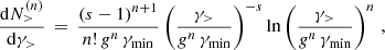 (A.5)
(A.5)
with n = nshock and g ∼ 2 in our scenario.
For electrons and protons accelerated on the same shock front, it can be shown that electrons will be preheated up to a fraction of equipartition as energy is transferred from protons to electrons. This leads to a relation between the minimum Lorentz factors γmin, e ∼ 600γmin, p. We suppose acceleration on mildly relativistic shocks with γsh ∼ 3, leading to γmin, p ∼ 3 and γmin, e ∼ 1800. An additional constraint comes from the fact that particles need to be able to scatter effectively in the microturbulence upstream and downstream of the shock front to allow repeated shock crossings and thus efficient energy gain. This leads to a relation between the minimum and maximum Lorentz factors that depends on the magnetisation σ:  .
.
To achieve acceptable representations of the observed SEDs within a coherent shock acceleration scenario, it is assumed that the magnetisation in the emission region downstream from the shock σrad can become orders of magnitude larger than the upstream magnetisation σ. This is justified through a possible amplification of the magnetic field caused by the flow of accelerated charged particles.
Given the low Lorentz factors of the proton population and its number density, which is equal to that of the electrons, any radiative emission from the protons, although fully modelled by the code, can be completely neglected. The presence of the proton population provides simply a physical justification for the high minimum Lorentz factors of the electrons.
A.3. OneHaLe
The ONEHALE code (Zacharias 2021; Zacharias et al. 2022) is a time-dependent, one-zone hadro-leptonic model calculating the particle distributions and photon spectra in a spherical region with radius R permeated by a tangled magnetic field B. It moves with bulk Lorentz factor Γ, and as above we assume here δ = Γ. The code contains various options for external fields, such as the accretion disk, the broad-line region, the dusty torus and the cosmic microwave background. However, in the application here, we do not consider the broad-line region or the dusty torus, and the accretion disk only serves as a potential contribution to the optical spectrum, but does not play a significant role in the particle–photon interactions.
The particle distribution ni(χ) of species i (protons, charged pions, muons, and electrons including positrons) is given here as a function of normalised momentum χ = pi/mic = γβ with the particle mass mi and  . The distributions are derived from the Fokker-Planck equation
![Mathematical equation: $$ \begin{aligned} \frac{\, \partial n_i(\chi ,t) \,}{\, \partial t \,}&= \frac{\, \partial \,}{\, \partial \chi \,} \left[ \frac{\chi ^2}{(a+2)t_{\rm acc}} \frac{\, \partial n_i(\chi ,t) \,}{\, \partial \chi \,} \right] - \frac{\, \partial \,}{\, \partial \chi \,} \left( \dot{\chi }_i n_i(\chi ,t) \right) \nonumber \\&\quad - \frac{n_i(\chi ,t)}{t_{\rm esc}} - \frac{n_i(\chi , t)}{\gamma t^{*}_{i,\mathrm{decay}}} + Q_i(\chi ,t) . \end{aligned} $$](/articles/aa/full_html/2024/02/aa48121-23/aa48121-23-eq57.gif) (A.6)
(A.6)
The first term on the right-hand-side describes Fermi-II acceleration through momentum diffusion employing hard-sphere scattering. The parameter a is the ratio of shock to Alvèn speed, while tacc is the energy-independent acceleration time scale. The second term contains continuous energy gains and losses. The gain is Fermi-I acceleration described by  , while the loss term contains the radiative and adiabatic processes of each particle species. All charged particles undergo synchrotron and adiabatic cooling, while protons additionally lose energy through Bethe-Heitler pair and pion production. We note that in the code version employed here, the conversion of protons to neutrons is not treated explicitly, but is considered as a continuous energy loss process instead. Electrons additionally undergo inverse-Compton losses, scattering all available internal and external photon fields.
The third term in Eq. (A.6) marks the escape of particles as in Sect. A.1. The fourth term describes the decay of unstable particles, which decay in proper time  . The final term contains the injection of particles. Primary injection of protons and electrons follows a simple power law as in Eq. (A.1) with normalisation
![Mathematical equation: $$ \begin{aligned} Q_{0,i}(t) = \frac{L_{\rm inj,i}(t)}{\frac{4}{3}\pi R^3 m_ic^2}\left[ \int \limits _{\gamma _{\rm min,i}}^{\gamma _{\rm max,i}}\, \mathrm{d} \gamma \, \gamma ^{1-s_i} \right]^{-1} . \end{aligned} $$](/articles/aa/full_html/2024/02/aa48121-23/aa48121-23-eq60.gif) (A.7)
(A.7)
We stress the fact that, in this case, the injection luminosity is given in the comoving frame, and therefore does not include the bulk Lorentz factor as in Eq. (A.4). The primary injection also includes primary acceleration indicating that the acceleration terms in Eq. (A.6) are merely acting as a mild reacceleration with tacc = ηacctesc. The pion injection term directly follows from the proton–photon interactions, while muons are injected from pion decay. Secondary electrons are injected from muon decay, Bethe-Heitler pair production, and γ-γ pair production. Neutral pions decay quickly into γ rays, which is why the resulting radiation is computed directly from their injection spectrum.
As Eq. (A.6) relies on the time-dependent photon spectrum present wihtin the emission region, in each time step we solve the Fokker-Planck equation for all charged particle species, and the radiation transport equation containing terms for photon production, absorption, and escape.
While the code is fully time-dependent, we use it here to calculate steady-state solutions. This is achieved if the total particle densities of protons np and electrons ne each vary less than 10−4 relative to the previous two time steps. The detailed equations of the whole code can be found in Zacharias et al. (2022).
Appendix B: Modelling parameters
In the following tables, we list the parameters of the various models employed in Sect. 4.3. In all tables, the particle injection luminosity in the SSC model is defined in the observer’s frame, while it is defined in the comoving frame in the other models.
Parameters for 1ES 0120+340 for the various models, input (top), inferred jet powers (bottom).
Parameters for RGB J0710+591 for the various models of Spectrum 1, input (top), inferred jet powers (bottom).
Parameters for RGB J0710+591 for the various models of Spectrum 2, input (top), inferred jet powers (bottom).
Parameters for RGB J0710+591 for the various models of Spectrum 3, input (top), inferred jet powers (bottom).
Parameters for 1ES 1101−232 for the various models, input (top), inferred jet powers (bottom).
Parameters for 1ES 1741+196 for the various models of Spectrum 1, input (top), inferred jet powers (bottom).
Parameters for 1ES 1741+196 for the various models of Spectrum 2, input (top), inferred jet powers (bottom).
Parameters for 1ES 1741+196 for the various models of Spectrum 3, input (top), inferred jet powers (bottom).
Parameters for 1ES 2322−409 for the various models, input (top), inferred jet powers (bottom).
All Tables
Best-fit log-parabola model parameters of joint SXT–LAXPC spectrum using TBabs*logpar model.
Source power-law indices of the SED in the optical/UV-to-X-ray part, αox, and the HE γ-ray part, αγ, as well as the time ranges and collected data sets for the modelling.
Total jet powers in erg s−1 for the various model fits, as well as the upper limit on the accretion disk power from the modelling.
Parameters for 1ES 0120+340 for the various models, input (top), inferred jet powers (bottom).
Parameters for RGB J0710+591 for the various models of Spectrum 1, input (top), inferred jet powers (bottom).
Parameters for RGB J0710+591 for the various models of Spectrum 2, input (top), inferred jet powers (bottom).
Parameters for RGB J0710+591 for the various models of Spectrum 3, input (top), inferred jet powers (bottom).
Parameters for 1ES 1101−232 for the various models, input (top), inferred jet powers (bottom).
Parameters for 1ES 1741+196 for the various models of Spectrum 1, input (top), inferred jet powers (bottom).
Parameters for 1ES 1741+196 for the various models of Spectrum 2, input (top), inferred jet powers (bottom).
Parameters for 1ES 1741+196 for the various models of Spectrum 3, input (top), inferred jet powers (bottom).
Parameters for 1ES 2322−409 for the various models, input (top), inferred jet powers (bottom).
All Figures
|
Fig. 1. Combined SXT and LAXPC-20 spectrum of 1ES 0120+340, RGB J0710+591 (A1: black; A2: red), 1ES 1101-232, 1ES 1741+196 (A1: black, A2: red; A3: green), and 1ES 2322-409(SXT only), (from left to right in top and bottom), fitted using the TBabs*logparabola model. |
| In the text | |
|
Fig. 2. Lightcurves of RGB J0710+591 overlaid with the Bayesian blocks representation. Top panel: Fermi-LAT in the energy range 0.3–300 GeV from 2008/09-2021/09 in 300-day bins in units of 10−9 cm−2 s−1. The upper limits correspond to 3σ limits. The dotted line represents the constant-fit. Bottom panel: Swift-XRT (in blue) and AstroSat-SXT (in black) in the energy range 0.3–7 keV in units of 10−11 erg cm−2 s−1. |
| In the text | |
|
Fig. 3. The MWL SEDs of 1ES 0120+340, RGB J0710+591, 1ES 1101–232, 1ES 1741+196, and 1ES 2322–409, respectively, with details given in the legends. The colored spectra follow the definition given in Table 4. |
| In the text | |
|
Fig. 4. Main (red) and archival (grey) data sets of 1ES 0120+340, as well as the various intrinsic models: SSC (red solid line), e-p-shock (magenta dash-double-dotted line), LHπ (blue dashed line), and LHp (orange dot-dashed line). The thin grey line marks the host galaxy template of Silva et al. (1998). |
| In the text | |
|
Fig. 5. Main (color) and archival (grey) data sets of RGB J0710+591, as well as the various intrinsic models (Top: for Spectrum 1 (black); Middle: for Spectrum 2 (blue); Bottom: for Spectrum 3 (red)): SSC (red solid line), e-p-shock (magenta dash-double-dotted line), LHπ (blue dashed line), and LHp (orange dot-dashed line). VHE γ-ray data have been corrected for EBL absorption. The thin grey line marks the host galaxy template of Silva et al. (1998). |
| In the text | |
|
Fig. 6. Main (red) and archival (grey) data sets of 1ES 1101−232, as well as the various intrinsic models: SSC (red solid line), e-p-shock (magenta dash-double-dotted line), LHπ (blue dashed line), and LHp (orange dot-dashed line). VHE γ-ray data have been corrected for EBL absorption. The thin grey line marks the host galaxy template of Silva et al. (1998). |
| In the text | |
|
Fig. 7. Main (colour) and archival (grey) data sets of 1ES 1741+196, as well as the various intrinsic models (Top: For Spectrum 1 (black). Middle: For Spectrum 2 (blue). Bottom: For Spectrum 3 (red)): SSC (red solid line), LHπ (blue dashed line), and LHp (orange dot-dashed line). VHE γ-ray data have been corrected for EBL absorption. The thin grey line marks the host galaxy template of Silva et al. (1998). |
| In the text | |
|
Fig. 8. Main (red) and archival (grey) data sets of 1ES 2322−409, as well as the various intrinsic models: SSC (red solid line), LHπ (blue dashed line), and LHp (orange dot-dashed line). VHE γ-ray data have been corrected for EBL absorption. |
| In the text | |
Current usage metrics show cumulative count of Article Views (full-text article views including HTML views, PDF and ePub downloads, according to the available data) and Abstracts Views on Vision4Press platform.
Data correspond to usage on the plateform after 2015. The current usage metrics is available 48-96 hours after online publication and is updated daily on week days.
Initial download of the metrics may take a while.