| Issue |
A&A
Volume 536, December 2011
|
|
|---|---|---|
| Article Number | A85 | |
| Number of page(s) | 25 | |
| Section | Cosmology (including clusters of galaxies) | |
| DOI | https://doi.org/10.1051/0004-6361/201117294 | |
| Published online | 15 December 2011 | |
Cosmic shear covariance: the log-normal approximation
1
Argelander-Institut für Astronomie, Universität Bonn,
Auf dem Hügel 71,
53121
Bonn,
Germany
e-mail: This email address is being protected from spambots. You need JavaScript enabled to view it.
2
Max-Planck-Institut für Astrophysik, Karl-Schwarzschild-Straße 1, 85741
Garching,
Germany
Received: 19 May 2011
Accepted: 18 October 2011
Abstract
Context. Accurate estimates of the errors on the cosmological parameters inferred from cosmic shear surveys require accurate estimates of the covariance of the cosmic shear correlation functions.
Aims. We seek approximations to the cosmic shear covariance that are as easy to use as the common approximations based on normal (Gaussian) statistics, but yield more accurate covariance matrices and parameter errors.
Methods. We derive expressions for the cosmic shear covariance under the assumption that the underlying convergence field follows log-normal statistics. We also derive a simplified version of this log-normal approximation by only retaining the most important terms beyond normal statistics. We use numerical simulations of weak lensing to study how well the normal, log-normal, and simplified log-normal approximations as well as empirical corrections to the normal approximation proposed in the literature reproduce shear covariances for cosmic shear surveys. We also investigate the resulting confidence regions for cosmological parameters inferred from such surveys.
Results. We find that the normal approximation substantially underestimates the cosmic shear covariances and the inferred parameter confidence regions, in particular for surveys with small fields of view and large galaxy densities, but also for very wide surveys. In contrast, the log-normal approximation yields more realistic covariances and confidence regions, but also requires evaluating slightly more complicated expressions. However, the simplified log-normal approximation, although as simple as the normal approximation, yields confidence regions that are almost as accurate as those obtained from the log-normal approximation. The empirical corrections to the normal approximation do not yield more accurate covariances and confidence regions than the (simplified) log-normal approximation. Moreover, they fail to produce positive-semidefinite data covariance matrices in certain cases, rendering them unusable for parameter estimation.
Conclusions. The log-normal or simplified log-normal approximation should be used in favour of the normal approximation for parameter estimation and parameter error forecasts. More generally, any approximation to the cosmic shear covariance should ensure a positive-(semi)definite data covariance matrix.
Key words: methods: numerical / large-scale structure of Universe / cosmological parameters / gravitational lensing: weak / cosmology: theory / methods: analytical
© ESO, 2011
1. Introduction
In recent years, observations of weak lensing by large-scale structure, called cosmic shear, have become an important tool for studying the Universe. Remarkable constraints on the matter content of the Universe, its expansion history, and the amplitude of the cosmic density fluctuations have been obtained, e.g., from measurements of cosmic shear in the Canada-France-Hawaii Telescope (CFHT) Legacy Survey (Semboloni et al. 2006; Hoekstra et al. 2006; Fu et al. 2008), the 100 deg2 weak-lensing survey (Benjamin et al. 2007), and the Cosmic Evolution Survey (COSMOS, Massey et al. 2007; Schrabback et al. 2010). Future cosmic shear surveys are expected to provide essential information on the properties of the dark matter and the dark energy, and on possible deviations of gravity from General Relativity (Huterer 2010).
Cosmic shear surveys aim at inferring the statistical properties of the convergence and shear field from the observed image shapes of distant galaxies. There are various statistical measures that probe the two-point statistics of the convergence and shear, e.g. the shear correlation functions (Blandford et al. 1991; Kaiser 1992), the shear power spectra (Kaiser 1992), the shear dispersion (Mould et al. 1994), the aperture-mass dispersion (Schneider et al. 1998), the ring statistics (Schneider & Kilbinger 2007), the statistics proposed by Fu & Kilbinger (2010), or the COSEBIs (Schneider et al. 2010). In practice, however, only the shear correlation functions ξ + and ξ− are estimated directly from the data (since they can be estimated most easily), and any other two-point statistics are computed from these estimates. Thus, accurate knowledge of the noise properties of the shear correlation estimators is needed for reliable estimates of the errors on the cosmological parameters inferred from cosmic shear surveys.
The number of independent measurements in a cosmic shear survey is usually too small to permit an good estimate of the full covariance of the measured statistics directly from the data. Therefore, one has to resort to covariance estimates obtained by other means. Supposedly the most accurate, but also computationally by far the most expensive approach is the direct estimation of a cosmic shear covariances from N-body simulations of cosmic structure formation (e.g. Sato et al. 2011b, or this work). This method requires many independent realisations of the survey field. So far, it has been successfully applied to lensing surveys covering a small fraction of the sky, e.g. the Chandra Deep Field South (Hartlap et al. 2009) and the COSMOS field (Schrabback et al. 2010; Semboloni et al. 2011). However, creating sufficiently many realistic mock observations to calculate covariances for future all-sky lensing surveys in various cosmologies and parameter ranges will remain a very challenging computational task in the foreseeable future.
Since reliable estimates for the covariances of cosmic shear two-point statistics from real or mock data are often out of reach, it appears desirable to have simple approximations at hand, which are easy to compute and yield sufficiently accurate covariance matrices and parameter errors. General expressions for the covariance of lensing two-point statistics, including the shear correlation functions, have been derived by Schneider et al. (2002a) and Joachimi et al. (2008) under the assumption of normal (Gaussian) statistics for the shear and convergence field. This normal approximation is relatively easy to apply, and requires no additional information besides the convergence correlation itself and the basic survey parameters. Simulations show, however, that the normal approximation tends to underestimate the covariance of two-point lensing statistics (e.g., Scoccimarro et al. 1999; Cooray & Hu 2001; Van Waerbeke et al. 2001; Sato et al. 2009).
There have been various attempts to improve the normal approximation by amending the resulting expressions for the cosmic shear covariance by scale-dependent correction factors that are calibrated with mock data from structure formation simulations (Van Waerbeke et al. 2001; Semboloni et al. 2007; Sato et al. 2011b). A drawback of this approach is that, while any corrections to the normal approximation depend in a non-trivial way on the assumed cosmology, the correction factors can only be tuned to the particular cosmology of the simulations at hand.
Other approaches towards more accurate lensing statistics are based on halo models (Cooray & Hu 2001; Takada & Jain 2009; Pielorz et al. 2010; Kainulainen & Marra 2011). The resulting expressions for the covariance of lensing two-point statistics require considerable more effort to compute than the corresponding expressions in the normal approximation, even if simplified by fitting formulas (Pielorz et al. 2010). A thorough assessment of the accuracy of the halo model approach to cosmic shear covariances (e.g. by comparing its results with those from large high-resolution simulations of weak lensing) is still outstanding.
Normal random fields are arguably the most simple statistical models for the three dimensional matter distribution and the resulting weak-lensing convergence and shear fields. However, as mentioned above, they fail to accurately describe those fields’ higher-order correlations such as the covariance of two-point correlations. There are few other classes of random fields that allow one to calculate their higher-order correlations analytically. These include log-normal random fields, on which we focus here.
Already Hubble (1934) noted that observed galaxy densities roughly follow a log-normal distribution. Coles & Jones (1991) suggested to describe the three-dimensional matter density distribution in our Universe by a log-normal random field. Later, numerical simulations of cosmic structure formation showed that a log-normal field provides indeed a good description of the one- and two-point statistics of the evolved matter density field, even though a point-wise exponential mapping of the initial Gaussian density field does not describe the evolved density field well (Kofman et al. 1994; Kayo et al. 2001). The one-point probability density function (pdf) of the projected density and lensing convergence are also fitted well by a log-normal pdf (Taruya et al. 2002). Even better fits to the convergence pdf, particularly in the tails of the distribution, can be obtained by generalisations of a log-normal pdf (Das & Ostriker 2006; Takahashi et al. 2011; Joachimi et al. 2011).
In this work, we derive expressions for the cosmic shear covariance under the assumption that the underlying convergence field follows log-normal statistics. Furthermore, we derive a simplified version of this log-normal approximation by only retaining the most important terms beyond normal statistics. In particular the simplified log-normal approximation meets our aim of an expression for the cosmic shear covariance that is as simple as the normal approximation.
We use numerical simulations to show that the log-normal and the simplified log-normal approximations reproduce the shear covariances for cosmic shear surveys much more accurately than the normal approximation. Furthermore, we demonstrate that, in contrast to the normal approximation, the uncertainties in the cosmological parameters inferred from the log-normal and the simplified log-normal approximation are in good agreement with the errors resulting from the covariances we estimated from the numerical simulations. We also show that the covariances and parameter errors in the log-normal approximation have accuracies comparable to or better than those derived from empirical corrections to the normal approximation proposed by Semboloni et al. (2007) and Sato et al. (2011b). In addition, we discuss the problem that approximations to the cosmic shear covariance, in particular those based on empirical fits, may produce covariance matrices that are not positive-semidefinite, which makes their use in parameter estimation at least questionable.
The paper is organised as follows. The theory of estimators for cosmic shear two-point statistics and their noise properties are briefly discussed in Sect. 2. In Sect. 3, we describe our numerical simulations for creating mock lensing surveys and for studying the statistical properties of the convergence and shear. The results of the simulations and the comparison between the different approximations to the cosmic shear covariance are presented in Sect. 4. The main part of the paper concludes with a summary and discussion in Sect. 5. A more detailed discussion about normal and log-normal random fields, and the covariance of estimators for the cosmic shear 2-point correlation can be found in the Appendix.
2. Theory
Here, we briefly discuss weak gravitational lensing, estimators for the cosmic shear correlation functions and their noise properties, and the estimation of cosmological parameters from cosmic shear data. The discussion of the statistical properties of the cosmic shear estimators is based on the real-space approach by Schneider et al. (2002a), but includes log-normal convergence fields in addition to normal convergence fields.
2.1. Gravitational lensing
Gravitational lensing, the deflection of photons from distant sources by the gravity of
intervening matter structures (e.g., Schneider et al.
2006), causes shifts in the observed image positions relative to the sources’ “true”
sky positions. The shifts may be described by a deflection field  (1)which relates the observed image position
θ = (θ1,θ2)
of a point-like source at redshift z to its true angular position
β = (β1(θ,z),β2(θ,z)).
The distortions induced by differential deflection can be quantified by the distortion matrix
(1)which relates the observed image position
θ = (θ1,θ2)
of a point-like source at redshift z to its true angular position
β = (β1(θ,z),β2(θ,z)).
The distortions induced by differential deflection can be quantified by the distortion matrix
 (2)which can be decomposed into a convergence
κ(θ,z), a complex shear
γ(θ,z) = γ1(θ,z) + iγ2(θ,z),
and an asymmetry ω(θ,z).
(2)which can be decomposed into a convergence
κ(θ,z), a complex shear
γ(θ,z) = γ1(θ,z) + iγ2(θ,z),
and an asymmetry ω(θ,z).
We define the effective convergence and shear for a population of sources with normalised
redshift distribution pz(z) by
![Mathematical equation: \begin{eqnarray} \label{eq:df_effective_convergence} \kappa(\vect{\theta}) &=& \int\idiff[]{z}\, p_z(z) \kappa(\vect{\theta}, z) ~~ {\rm and} \\ \label{eq:df_effective_shear} \gamma(\vect{\theta}) &=& \int\idiff[]{z}\, p_z(z) \gamma(\vect{\theta}, z). \end{eqnarray}](/articles/aa/full_html/2011/12/aa17294-11/aa17294-11-eq16.png) The tangential component
γt(θ,ϑ)
and cross component
γ × (θ,ϑ)
of the shear γ(θ) at
position θ with respect to the direction
ϑ are defined by (e.g., Schneider et al. 2002b)
The tangential component
γt(θ,ϑ)
and cross component
γ × (θ,ϑ)
of the shear γ(θ) at
position θ with respect to the direction
ϑ are defined by (e.g., Schneider et al. 2002b)  where
ϕ(ϑ) denotes the polar angle of the
vector ϑ.
where
ϕ(ϑ) denotes the polar angle of the
vector ϑ.
For a statistically homogeneous and isotropic universe, the convergence correlation function
ξκ(ϑ) can be defined by the
expectation (e.g., Blandford et al. 1991; Kaiser 1992)
 (7a)Here, ⟨f⟩ denotes the ensemble
average of a function f over all realisations of the observable universe for a
fixed set of cosmological parameters. The two shear correlation
functions ξ + (ϑ)
and ξ−(ϑ) are defined by
(7a)Here, ⟨f⟩ denotes the ensemble
average of a function f over all realisations of the observable universe for a
fixed set of cosmological parameters. The two shear correlation
functions ξ + (ϑ)
and ξ−(ϑ) are defined by
 (7b)If one neglects higher-order lensing effects (which
are small, cf. Hilbert et al. 2009; Krause & Hirata 2010) and contamination by observational
systematics, the deflection field (1) is a
gradient field, the asymmetry ω vanishes, and the
convergence κ and shear γ are related by (Kaiser 1995)
(7b)If one neglects higher-order lensing effects (which
are small, cf. Hilbert et al. 2009; Krause & Hirata 2010) and contamination by observational
systematics, the deflection field (1) is a
gradient field, the asymmetry ω vanishes, and the
convergence κ and shear γ are related by (Kaiser 1995)  (8)As a consequence (Crittenden et al. 2002),
 ![Mathematical equation: \begin{eqnarray} \label{eq:xi_p_from_xi_kappa} \xi_+ (\vartheta) &=& \xi_{\kappa} (\vartheta) ~~{\rm and} \\ \label{eq:xi_m_from_xi_kappa} \xi_- (\vartheta) &=& \int_0^{\infty}\idiff[]{\vartheta'}\,\vartheta' \KerM (\vartheta,\vartheta') \xi_{\kappa} (\vartheta'), \end{eqnarray}](/articles/aa/full_html/2011/12/aa17294-11/aa17294-11-eq35.png) where
where  (11)Here, H denotes the Heaviside step
function, and δD denotes the Dirac delta function.
(11)Here, H denotes the Heaviside step
function, and δD denotes the Dirac delta function.
2.2. Estimators for the shear correlations and their covariance
A suitable estimator for the shear
γ(θ(i)) at the sky
position θ(i) of a
galaxy i at redshift z(i) from a
sample with redshift
distribution pz(z) is the
observed image ellipticity  .
To lowest order, the observed ellipticity is a sum,
.
To lowest order, the observed ellipticity is a sum,
 (12)of the “true” shear
γ(θ(i),z(i))
and an intrinsic ellipticity ϵ(i), which vanishes
on average. From a survey with Ng galaxies providing shear
estimates
(12)of the “true” shear
γ(θ(i),z(i))
and an intrinsic ellipticity ϵ(i), which vanishes
on average. From a survey with Ng galaxies providing shear
estimates  at positions
θ(1),...,θ(N),
one can estimate the shear correlations ξ ± (ϑ) at
separations ϑ by1
at positions
θ(1),...,θ(N),
one can estimate the shear correlations ξ ± (ϑ) at
separations ϑ by1 (13)Here, the bin window function
  (14)where Δ(ϑ) denotes
the bin width, and
(14)where Δ(ϑ) denotes
the bin width, and  and
and  denote the tangential and cross component,
respectively, of the shear estimated from the shape of galaxy i with respect
to the line joining galaxy i and j.
denote the tangential and cross component,
respectively, of the shear estimated from the shape of galaxy i with respect
to the line joining galaxy i and j.
If (i) the bin width is small compared to the scales on which correlations change; (ii) the
galaxy positions are not correlated with the shear field; (iii) the galaxy redshifts are not
correlated with each other or the shear field; and (iv) the galaxies’ intrinsic ellipticities
are uncorrelated with each other and the shear, the estimators (13) are unbiased (Schneider et al.
2002a),  (15)The covariance of the cosmic shear estimators
determines the accuracy to which one can deduce cosmological parameters from these estimators.
The covariance
(15)The covariance of the cosmic shear estimators
determines the accuracy to which one can deduce cosmological parameters from these estimators.
The covariance  of the estimators (13) for
scales ϑ1 and ϑ2 can then be split
into an ellipticity-noise part
of the estimators (13) for
scales ϑ1 and ϑ2 can then be split
into an ellipticity-noise part  , a mixed part
 , and a cosmic variance part
 :
:  (16)First, we consider the covariance for a single
survey field F with area AF, galaxy density
ng = Ng/AF,
and linear dimensions large compared to ϑ1 and
ϑ2. The ellipticity-noise part
(16)First, we consider the covariance for a single
survey field F with area AF, galaxy density
ng = Ng/AF,
and linear dimensions large compared to ϑ1 and
ϑ2. The ellipticity-noise part
 vanishes for c+−,
and for disjoint bins. Its contribution to the auto-variance of the bin with radius
ϑ depends on the variance
vanishes for c+−,
and for disjoint bins. Its contribution to the auto-variance of the bin with radius
ϑ depends on the variance  of the intrinsic ellipticity and the expected
effective number of galaxy pairs
of the intrinsic ellipticity and the expected
effective number of galaxy pairs  in the bin,
  (17)The mixed part
 contributes to both the auto- and covariance of
bins:
contributes to both the auto- and covariance of
bins: ![Mathematical equation: % subequation 1389 0 \begin{eqnarray} c^{(\epsilon\gamma)}_{++}\left(\vartheta_1, \vartheta_2 \right) &=& \frac{2\sigmaepsilongal^2}{\pi\ngal \AFOV} \int_{0}^{\pi}\!\!\idiff[]{\varphi_1}\, \xi_+\bigl(\lvert \vartheta_2 \uvect{0} - \vartheta_1 \uvect{\varphi_1} \rvert\bigr), \end{eqnarray}](/articles/aa/full_html/2011/12/aa17294-11/aa17294-11-eq75.png) (18a)
(18a)![Mathematical equation: % subequation 1389 1 \begin{eqnarray} c^{(\epsilon\gamma)}_{+-}\left(\vartheta_1, \vartheta_2 \right) &=& \frac{2\sigmaepsilongal^2}{\pi\ngal \AFOV} \int_{0}^{\pi}\!\!\idiff[]{\varphi_1}\, \xi_-\bigl(\lvert \vartheta_2 \uvect{0} - \vartheta_1 \uvect{\varphi_1} \rvert\bigr)\nonumber\\ &&\quad\times \cos\left[4\varphi(\vartheta_2 \uvect{0} - \vartheta_1 \uvect{\varphi_1} )\right] {\rm , and} \end{eqnarray}](/articles/aa/full_html/2011/12/aa17294-11/aa17294-11-eq76.png) (18b)
(18b)![Mathematical equation: % subequation 1389 2 \begin{eqnarray} c^{(\epsilon\gamma)}_{--}\left(\vartheta_1, \vartheta_2 \right) &=& \frac{2\sigmaepsilongal^2}{\pi\ngal \AFOV} \!\! \int_{0}^{\pi}\!\!\idiff[]{\varphi_1} \, \xi_+\bigl(\lvert \vartheta_2 \uvect{0} - \vartheta_1 \uvect{\varphi_1} \rvert\bigr) \cos(4\varphi_1). \end{eqnarray}](/articles/aa/full_html/2011/12/aa17294-11/aa17294-11-eq77.png) (18c)Here,
uϕ denotes a unit vector in the
plane with polar angle ϕ.
(18c)Here,
uϕ denotes a unit vector in the
plane with polar angle ϕ.
Calculating the cosmic variance part  requires knowledge about the 4-point statistics
of the convergence field. If one assumes that the convergence field is a homogeneous and
isotropic normal random field, the cosmic variance parts read (Schneider et al. 2002a)
requires knowledge about the 4-point statistics
of the convergence field. If one assumes that the convergence field is a homogeneous and
isotropic normal random field, the cosmic variance parts read (Schneider et al. 2002a) ![Mathematical equation: \begin{eqnarray} \label{eq:c_gamma_normal} c^{(\gamma)}_{\pm\pm}\left(\vartheta_1, \vartheta_2 \right) &= & \frac{4}{\pi\AFOV}\!\int_{0}^{\rFOV}\idiff[]{\theta_3}\, \theta_3 \int_{0}^{\pi}\idiff[]{\varphi_1}\, \zeta_{\pm}\bigl( \vartheta_1 \uvect{\varphi_1}, \theta_3 \uvect{0} \bigr) \nonumber\\[2mm] &&\quad \times \!\int_{0}^{\pi}\idiff[]{\varphi_2}\, \zeta_{\pm}\bigl( \vartheta_2 \uvect{\varphi_2}, \theta_3 \uvect{0} \bigr) \end{eqnarray}](/articles/aa/full_html/2011/12/aa17294-11/aa17294-11-eq81.png) (19)where
(19)where ![Mathematical equation: % subequation 1463 0 \begin{eqnarray} \zeta_{+}\left( \vtheta, \vtheta' \right) &=& \xi_{+}(\lvert \vtheta' - \vtheta \rvert),\\ \zeta_{-}\left( \vtheta, \vtheta' \right) &=& \xi_{-}(\lvert \vtheta' - \vtheta \rvert) \cos\left[\varphi(\vtheta) - \varphi(\vtheta' - \vtheta) \right], \end{eqnarray}](/articles/aa/full_html/2011/12/aa17294-11/aa17294-11-eq82.png) and
and  denotes the “radius” of the survey field, a scale
similar to the field’s linear dimensions2.
denotes the “radius” of the survey field, a scale
similar to the field’s linear dimensions2.
In this work, we also consider zero-mean shifted log-normal random fields (see Appendix for
details) as models for the convergence field. Such a field κ can be obtained
from a homogeneous and isotropic normal random field n with
mean μ and standard deviation σ by the point-wise
transformation ![Mathematical equation: \begin{equation} \kappa(\vtheta) = \exp\bigl[n(\vtheta)\bigr] - \kappa_0, \end{equation}](/articles/aa/full_html/2011/12/aa17294-11/aa17294-11-eq87.png) (21)which implies a zero-mean shifted log-normal pdf,
(21)which implies a zero-mean shifted log-normal pdf,
![Mathematical equation: \begin{equation} p_\kappa(\kappa) = \begin{cases} \dfrac{\exp\Biggl\{-\dfrac{\bigl[\ln(\kappa / \kappa_0 + 1) + \sigma^2/2 \bigr]^2}{2\sigma^2}\Biggl\} }{\sqrt{2\pi}(\kappa + \kappa_0)\sigma} & {\rm for }\;\; \kappa > -\kappa_0, \\[3mm] 0 & {\rm otherwise.} \end{cases} \label{eq:zero_mean_shifted_log_normal_kappa_pdf} \end{equation}](/articles/aa/full_html/2011/12/aa17294-11/aa17294-11-eq88.png) (22)Choosing the shift
κ0 = exp(μ + σ2/2)
ensures zero mean. Since −κ0 marks the lower limit for all
possible κ, we call κ0 minimum-convergence
parameter.
(22)Choosing the shift
κ0 = exp(μ + σ2/2)
ensures zero mean. Since −κ0 marks the lower limit for all
possible κ, we call κ0 minimum-convergence
parameter.
If the convergence field is well described by a zero-mean shifted log-normal random field,
the cosmic variance term  of the cosmic shear covariance reads (see
Appendix C)
of the cosmic shear covariance reads (see
Appendix C) ![Mathematical equation: \begin{eqnarray} && c^{(\gamma)}_{++}\left(\vartheta_1, \vartheta_2 \right) = \xi_{+}(\vartheta_1) \xi_{+}(\vartheta_2) \frac{8 \pi}{\kappa_0^{2}\AFOV} \int_{0}^{\rFOV}\iidiff[]{\theta_3}\, \theta_3\, \xi_{+}(\theta_3) \nonumber\\&& \quad +\, \frac{4 \eta(\vartheta_1) \xi_{+}(\vartheta_2)}{\kappa_0^2\AFOV} \int_{0}^{\rFOV}\iidiff[]{\theta_3}\, \theta_3\, \xi_{+}(\theta_3) \int_{0}^{\pi}\iidiff[]{\varphi_1}\, \xi_{+}(\lvert \theta_3\uvect{0} - \vartheta_1\uvect{\varphi_1} \rvert) \nonumber\\&& \quad +\, \frac{4 \xi_{+}(\vartheta_1) \eta(\vartheta_2)}{\kappa_0^2\AFOV} \int_{0}^{\rFOV}\iidiff[]{\theta_3}\, \theta_3\, \xi_{+}(\theta_3) \int_{0}^{\pi}\iidiff[]{\varphi_2}\, \xi_{+}(\lvert \theta_3\uvect{0} - \vartheta_2\uvect{\varphi_2} \rvert) \nonumber\\ && \quad +\, \frac{\eta(\vartheta_1)\eta(\vartheta_2)}{2\pi \AFOV} \int_{0}^{\rFOV}\idiff[]{\theta_3}\,\theta_3 \int_{0}^{2\pi}\idiff[]{\varphi_1} \int_{0}^{2\pi}\idiff[]{\varphi_2}\, \nonumber\\&& \quad \times\, \xi_{+}(\lvert \theta_3\uvect{0} - \vartheta_1\uvect{\varphi_1} \rvert) \xi_{+}(\lvert \theta_3\uvect{0} - \vartheta_2\uvect{\varphi_2} \rvert) \nonumber \\&& \quad \times \, \Bigl[ 2 \!+\! 4 \kappa_0^{-2} \xi_{+}(\theta_3) \!+\!\kappa_0^{-4} \xi_{+}(\theta_3) \xi_{+}(\lvert \theta_3\uvect{0} \!-\! \vartheta_1\uvect{\varphi_1}\! -\! \vartheta_2\uvect{\varphi_2} \rvert) \Bigr] \label{eq:c_gamma_pp_log_normal} \end{eqnarray}](/articles/aa/full_html/2011/12/aa17294-11/aa17294-11-eq93.png) (23) with
(23) with
 . We are unable to derive equally “concise”
expressions for the cosmic variance parts
. We are unable to derive equally “concise”
expressions for the cosmic variance parts  and
and  . However, and can be obtained from any given
by an integral transformation with the
kernel (11) (see Appendix C):
. However, and can be obtained from any given
by an integral transformation with the
kernel (11) (see Appendix C): ![Mathematical equation: \begin{eqnarray} \label{eq:c_pp_to_pm}c^{(\gamma)}_{+-}(\vartheta_1,\vartheta_2) &=& \int_0^{\infty}\idiff[]{\vartheta'_2}\,\vartheta'_2\, \KerM (\vartheta_2,\vartheta'_2)c^{(\gamma)}_{++}(\vartheta_1,\vartheta'_2), \\ c^{(\gamma)}_{--}(\vartheta_1,\vartheta_2) &=& \int_0^{\infty}\idiff[]{\vartheta'_1}\,\vartheta'_1\, \KerM(\vartheta_1,\vartheta'_1) \int_0^{\infty}\idiff[]{\vartheta'_2}\,\vartheta'_2\, \KerM(\vartheta_2,\vartheta'_2) \nonumber\\ \label{eq:c_pp_to_mm} &&\quad\times c^{(\gamma)}_{++}(\vartheta'_1,\vartheta'_2). \end{eqnarray}](/articles/aa/full_html/2011/12/aa17294-11/aa17294-11-eq97.png) Equation (23) comprises terms of 2nd to 6th order in
ξκ. If only the quadratic terms, which are also
present in the expression (19), and the
simplest cubic term in ξκ are retained, the cosmic
variance contribution reduces to
Equation (23) comprises terms of 2nd to 6th order in
ξκ. If only the quadratic terms, which are also
present in the expression (19), and the
simplest cubic term in ξκ are retained, the cosmic
variance contribution reduces to ![Mathematical equation: \begin{eqnarray} \label{eq:c_gamma_simplified_log_normal} c^{(\gamma)}_{\pm\pm}\left(\vartheta_1, \vartheta_2 \right) &= & \frac{4}{\pi\AFOV}\!\int_{0}^{\rFOV}\idiff[]{\theta_3}\, \theta_3\, \!\int_{0}^{\pi}\idiff[]{\varphi_1}\, \zeta_{\pm}\bigl( \vartheta_1 \uvect{\varphi_1}, \theta_3 \uvect{0} \bigr) \nonumber \\ &&\quad\times \!\int_{0}^{\pi}\idiff[]{\varphi_2}\, \zeta_{\pm}\bigl( \vartheta_2 \uvect{\varphi_2}, \theta_3 \uvect{0} \bigr) \nonumber \\ &&\quad + \xi_{\pm}(\vartheta_1) \xi_{\pm}(\vartheta_2)\frac{8 \pi}{\kappa_0^{2}\AFOV} \int_{0}^{\rFOV}\idiff[]{\theta_3}\,\theta_3\, \xi_{+}(\theta_3). \end{eqnarray}](/articles/aa/full_html/2011/12/aa17294-11/aa17294-11-eq99.png) (26)In the following, we call the approximation defined
by Eqs. (16)−(19) the normal approximation to the cosmic shear covariance. If Eqs. (23)−(25) are used instead of Eq. (19), we
call the resulting approximation to the cosmic shear covariance the log-normal approximation.
If Eq. (26) is used instead, we call the
resulting approximation the simplified log-normal approximation.
(26)In the following, we call the approximation defined
by Eqs. (16)−(19) the normal approximation to the cosmic shear covariance. If Eqs. (23)−(25) are used instead of Eq. (19), we
call the resulting approximation to the cosmic shear covariance the log-normal approximation.
If Eq. (26) is used instead, we call the
resulting approximation the simplified log-normal approximation.
In general, the convergence field is neither a normal nor a zero-mean shifted log-normal
field. In case one has a large sample of Nr (quasi-)independent
realisations of the survey field with measured correlations
 , one can estimate the mean using the sample mean,
 (27)and the covariance using the sample covariance,
![Mathematical equation: \begin{equation} c_{\pm\pm}\left(\vartheta_1, \vartheta_2 \right) = \frac{1}{N_{\rm r} - 1}\!\!\sum_{r=1}^{N_{\rm r}} \bigl[\est{\xi}_\pm^r(\vartheta_1) - \est{\xi}_\pm(\vartheta_1)\bigr] \bigl[\est{\xi}_\pm^r(\vartheta_2) - \est{\xi}_\pm(\vartheta_2)\bigr]. \end{equation}](/articles/aa/full_html/2011/12/aa17294-11/aa17294-11-eq104.png) (28)For many surveys, the survey area is not a single
field, but consists of several small areas that are far apart from each other on the sky. In
this case, the measurements in each field can be considered independent from the measurements
in the other fields. If all survey fields have similar field areas and galaxy densities, the
covariances for the whole survey can be obtained by computing the covariances for a single
field and dividing the result by the number of fields.
(28)For many surveys, the survey area is not a single
field, but consists of several small areas that are far apart from each other on the sky. In
this case, the measurements in each field can be considered independent from the measurements
in the other fields. If all survey fields have similar field areas and galaxy densities, the
covariances for the whole survey can be obtained by computing the covariances for a single
field and dividing the result by the number of fields.
2.3. Estimation of cosmological parameters
From a set of shear correlation functions
ξ ± (ϑ1),...,ξ ± (ϑNbins)
measured at Nbins angular separations, one can form a data vector
 (29)In one of its simplest forms, Bayesian
model-parameter estimation from a measured cosmic shear data
vector d amounts to a maximum likelihood parameter estimation
assuming a quadratic log-likelihood
(29)In one of its simplest forms, Bayesian
model-parameter estimation from a measured cosmic shear data
vector d amounts to a maximum likelihood parameter estimation
assuming a quadratic log-likelihood ![Mathematical equation: \begin{equation} \loglikelihood(\vect{\pi}|\vect{d}) = -\frac{1}{2}\transposed{\left[\vect{d} - \vect{\mu}(\vect{\pi}) \right]} \matrb{C}_{\rm d}^{-1} \left[\vect{d} - \vect{\mu}(\vect{\pi}) \right] +{\rm const.} \label{eq:quadratic_log_likelihood} \end{equation}](/articles/aa/full_html/2011/12/aa17294-11/aa17294-11-eq109.png) (30)Here,
μ(π) denotes the prediction of
the cosmic shear correlation vector for the model characterized by a set of
Np parameters
π = (π1,...,πNp)t.
If one uses the normal or log-normal approximation to the cosmic shear covariance, the inverse
covariance matrix
(30)Here,
μ(π) denotes the prediction of
the cosmic shear correlation vector for the model characterized by a set of
Np parameters
π = (π1,...,πNp)t.
If one uses the normal or log-normal approximation to the cosmic shear covariance, the inverse
covariance matrix  of the data
vector d reads:
of the data
vector d reads: 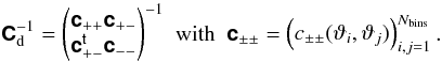 (31)If the cosmic shear covariances
c ± ± are estimated from the sample covariances of
Nr realisations, the inverse covariance can be estimated by (Anderson 2003; Hartlap et al.
2007)
(31)If the cosmic shear covariances
c ± ± are estimated from the sample covariances of
Nr realisations, the inverse covariance can be estimated by (Anderson 2003; Hartlap et al.
2007)  (32)where the correction factor ensures that this
estimate is unbiased if the joint distribution of the measured correlation functions is well
approximated by a multivariate normal distribution. This estimate requires
Nr > (2Nbins + 2).
For smaller Nr, the sample covariance matrix is not invertible, and
other methods are required to estimate the inverse covariance matrix.
(32)where the correction factor ensures that this
estimate is unbiased if the joint distribution of the measured correlation functions is well
approximated by a multivariate normal distribution. This estimate requires
Nr > (2Nbins + 2).
For smaller Nr, the sample covariance matrix is not invertible, and
other methods are required to estimate the inverse covariance matrix.
The parameter set πML maximizing the
(log-)likelihood satisfies ![Mathematical equation: \begin{equation} \vect{0} = \transposed{\left.\parder{\vect{\mu}(\vect{\pi})}{\vect{\pi}}\right|_{\vect{\pi}_{\rm ML}}} \matrb{C}_{\rm d}^{-1} \left[\vect{d} - \vect{\mu}(\vect{\pi}_{\rm ML}) \right]. \end{equation}](/articles/aa/full_html/2011/12/aa17294-11/aa17294-11-eq119.png) (33)A Taylor expansion of
lnL(π|d)
around πML up to second order yields
(33)A Taylor expansion of
lnL(π|d)
around πML up to second order yields 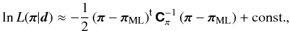 (34)where
![Mathematical equation: \begin{equation} \matrb{C}_{\pi}^{-1} = \begin{pmatrix} \displaystyle\sum_{k,l=1}^{\NBins} \matr{C}^{-1}_{{\rm d},kl} \left[ \dparder{\mu_k}{\pi_i} \dparder{\mu_l}{\pi_j} + (d_k - \mu_k) \dparder{^2 \mu_k}{\pi_i \partial \pi_j} \right]_{\vect{\pi}_{\rm ML}} \end{pmatrix}_{i,j = 1}^{N_{\rm p}} \end{equation}](/articles/aa/full_html/2011/12/aa17294-11/aa17294-11-eq122.png) (35)differs from the Fisher matrix by additional
contributions from second derivatives of μ when
μ(πML) ≠ d.
(35)differs from the Fisher matrix by additional
contributions from second derivatives of μ when
μ(πML) ≠ d.
The equations above show how the covariances and confidence regions of the model parameters
depend on the assumed covariances of the cosmic shear correlation functions in a
maximum-likelihood estimation with a Gaussian likelihood. In a Bayesian analysis with constant
priors on the model parameters, the
likelihood L(π|d)
is proportional to the posterior
distribution p(π|d).
In this case, the above equations also specify how the posterior distribution depends on the
assumed covariance of the cosmic shear correlation functions. For more general prior
distributions p(π), the posterior reads
![Mathematical equation: \begin{equation} p(\vect{\pi}|\vect{d}) = \frac{\likelihood (\vect{\pi}|\vect{d}) p(\vect{\pi})}{ \int\diff[N_{\rm p}]{\vect{\pi}}\, \likelihood (\vect{\pi}|\vect{d}) p(\vect{\pi})}\cdot \label{eq:general_posterior} \end{equation}](/articles/aa/full_html/2011/12/aa17294-11/aa17294-11-eq128.png) (36)
(36)
3. Simulations
We use a numerical approach to assess the performance of predictions for the cosmic shear covariance. By ray-tracing through the Millennium Run (MR), a large N-body simulation of cosmic structure formation by Springel et al. (2005), we create a suite of simulated fields of view with maps of the effective convergence and shear. From these maps, we measure the convergence distribution and the convergence and shear correlations. We then estimate the covariance of the shear correlation functions in different ways: from the measured one- and two-point statistics of the convergence using the normal, log-normal, and simplified log-normal approximation, and from the sample covariance of the shear correlation in the simulated survey fields.
The MR assumes a flat ΛCDM cosmology with a matter density Ωm = 0.25, a baryon density Ωb = 0.045, and a cosmological-constant energy density ΩΛ = 0.75 (in units of the critical density), a Hubble constant h = 0.73 (in units of 100 km s-1 Mpc-1), a primordial spectral index ns = 1 and a normalisation parameter σ8 = 0.9 for the linear density power spectrum. These values also define our fiducial cosmology in the later analysis. The simulation employed a customized version of gadget-2 (Springel 2005) with 1010 particles of 8.6 × 10⁸ h-1 M⊙ in a cube of 500 h-1 Mpc comoving side length, and a comoving force softening length of 5 h-1 kpc.
We employ the multiple-lens-plane ray-tracing algorithm described in Hilbert et al. (2009) to simulate gravitational lensing observations. The ray-tracing algorithm takes into account the gravitational deflection by the dark matter, represented by the dark-matter particles of the MR, and the deflection by the stellar mass in galaxies (for details, see Hilbert et al. 2008) as inferred from the galaxy-formation model of De Lucia & Blaizot (2007).
Using the ray-tracing, we generate 64 fields of view. Each field has an area of 4 × 4 deg2 (yielding a total area of 1024 deg2) and is covered by a regular grid of 40962 pixels (yielding a resolution of 3.5 arcsec). For each pixel, a ray is traced through the MR up to redshift 3.2, and the convergence and shear along the ray is recorded. To study the covariance of smaller survey fields, we also create 256 fields of 2 × 2 deg2 by splitting the 4 × 4 deg2 fields evenly.
The convergence and shear information along the rays is then used to calculate the effective
convergence and shear in the simulated fields for a source population with median redshift
zmedian = 1 and a redshift distribution (Brainerd et al. 1996) ![Mathematical equation: \begin{equation} p_{z}(z)=\frac{3z^2}{2z_0^3}\exp\left[-\left(\frac{z}{z_0}\right)^{3/2} \right],\;\; {\rm where }\; z_0 = \frac{z_{\rm median}}{1.412}\cdot \label{eq:source_redshift_distribution} \end{equation}](/articles/aa/full_html/2011/12/aa17294-11/aa17294-11-eq151.png) (37)The only source of noise (i.e. uncertainties
affecting the estimation of cosmological parameters) in these ellipticity noise-free maps is the
cosmic variance (each field represents only a single finite realization of the underlying
cosmology). To create noisy lensing maps that also incorporate the uncertainties in cosmic shear
surveys arising from the intrinsic shapes of source galaxies, we add Gaussian noise with
standard deviation
(37)The only source of noise (i.e. uncertainties
affecting the estimation of cosmological parameters) in these ellipticity noise-free maps is the
cosmic variance (each field represents only a single finite realization of the underlying
cosmology). To create noisy lensing maps that also incorporate the uncertainties in cosmic shear
surveys arising from the intrinsic shapes of source galaxies, we add Gaussian noise with
standard deviation 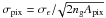 to each pixel (with pixel area
Apix ≈ 3.52 arcsec2) of the simulated shear
fields. We assume an intrinsic galaxy ellipticity distribution with standard deviation
σϵ = 0.4, and we consider surveys with galaxy
densities ng = 25 arcmin-2 and
ng = 100 arcmin-2.
to each pixel (with pixel area
Apix ≈ 3.52 arcsec2) of the simulated shear
fields. We assume an intrinsic galaxy ellipticity distribution with standard deviation
σϵ = 0.4, and we consider surveys with galaxy
densities ng = 25 arcmin-2 and
ng = 100 arcmin-2.
4. Results
4.1. The convergence distribution
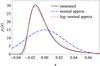 |
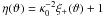
Fig. 1 The pdf pκ(κ) of the convergence κ for sources with median redshift zmedian = 1. The pdf measured from the simulations (solid line) is compared to a zero-mean normal distribution with matching variance (dashed line), and the best-fitting zero-mean shifted log-normal distribution (dotted line). |
We determine the convergence distribution from the simulated fields by binning the ellipticity noise-free convergence values of all field pixels into bins of size 0.002. The resulting probability density function (pdf) of the convergence distribution is shown Fig. 1. For comparison, we also show the pdf of a zero-mean normal distribution, whose variance equals the measured variance of the convergence, and the pdf (22) of the best-fitting zero-mean shifted log-normal distribution, whose parameters κ0 and σ where obtained by a simple least-squares fit. Neither the normal nor the zero-mean shifted log-normal distribution matches the measured convergence distribution perfectly, but (at least visually) the zero-mean shifted log-normal distribution fares far better than the normal distribution. This finding indicates that the log-normal approximation might possibly provide a better approximation to the covariance of the cosmic shear correlation than the normal approximation.
While the normal approximation to the covariance of cosmic shear correlations only needs the convergence correlation as input, the log-normal approximation also requires the minimum-convergence parameter κ0. One could, for example, compute the convergence for an empty beam to a fixed source redshift and use its modulus as κ0. Simulations show, however, that there are no empty lines of sight in a ΛCDM universe (Taruya et al. 2002; Vale & White 2003; Hilbert et al. 2007). We thus use the value κ0 ≈ 0.032 obtained from the fit (22).
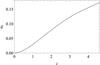 |
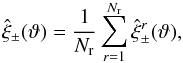
Fig. 2 The minimum-convergence parameter κ0 as a function of source redshift z (obtained from fits to the pdf of the convergence for sources at redshift z). |
The minimum-convergence parameter κ0(z) for sources at a single redshift z, obtained from fits to the measured pdf of the convergence κ(z), is shown in Fig. 2 as a function of source redshift and listed in Table 1 along with the second fit parameter σ and the standard deviation of the convergence. The parameter σ can be interpreted as a measure of non-Gaussianity of the convergence field. The values 0.5 ≲ σ ≲ 1 indicate a moderate degree of non-Gaussianity (Martin et al. 2011).
The redshift dependence of κ0 in the range
0.3 ≤ z ≤ 4 is well described by
 (38)The minimum-convergence parameter for sources at
redshift z = 1 is very similar to the value measured from the source redshift
distribution (37) with median redshift
zmedian = 1. Moreover, the minimum-convergence for
z = 1 and z = 2 are in good agreement with the corresponding
values found by Taruya et al. (2002).
(38)The minimum-convergence parameter for sources at
redshift z = 1 is very similar to the value measured from the source redshift
distribution (37) with median redshift
zmedian = 1. Moreover, the minimum-convergence for
z = 1 and z = 2 are in good agreement with the corresponding
values found by Taruya et al. (2002).
4.2. The convergence and shear correlations
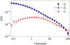 |
Fig. 3 The convergence correlation ξκ(ϑ) (squares) and the cosmic shear correlations ξ + (ϑ) (diamonds) and ξ−(ϑ) (triangles) as functions of the angular scale ϑ for sources with median redshift zmedian = 1 measured from the simulations. Error bars indicate uncertainties on the mean estimated from the field-to-field variance of the simulated fields. Also shown are the analytic fits (see text) to the correlations ξ + (ϑ) (dashed line) and ξ−(ϑ) (dotted line). |
From each ellipticity noise-free simulated 4 × 4 deg2 field, we estimate the convergence correlation ξκ(θ) and the cosmic shear correlations ξ ± using fast Fourier transform (FFT) techniques employing zero-padding and book-keeping of the number of contributing pixel pairs to properly account for the non-periodic field boundaries (see Appendix D for more details). The correlation estimates from all fields are then used to compute the mean correlations and their uncertainties from the field-to-field variance.
The resulting convergence and cosmic shear correlations are shown in Fig. 3. As expected, the measured shear correlation ξ + is almost identical to the measured convergence correlation ξκ. Numerical tests verify furthermore that the measured correlations ξκ and ξ− satisfy the relation (10) well within the error bars.
Computation of the covariance of the cosmic shear correlations in the (log-)normal
approximation involves integrals over the shear correlations. To facilitate the integration, we
approximate the measured correlation functions ξ ± by analytic
expressions  with parameters a1,
a2, b1,
b2, b3, τ1,
τ2, and τ3 obtained from a weighted
least-squared fit. The resulting expressions fit the measured correlations very well,
as Fig. 3 shows.
with parameters a1,
a2, b1,
b2, b3, τ1,
τ2, and τ3 obtained from a weighted
least-squared fit. The resulting expressions fit the measured correlations very well,
as Fig. 3 shows.
4.3. The covariance of the cosmic shear correlation functions
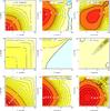 |
Fig. 4 The cosmic variance contributions |
We estimate the cosmic variance contribution to the cosmic shear covariance from the sample
covariance (27) of the measured shear
correlation functions in the ellipticity noise-free simulated fields.
Furthermore, we calculate estimates for within the normal approximation and the
log-normal approximation, using the fits (39b) as inputs for the shear correlation functions. The estimates from the sample
covariance of the 2 × 2 deg2 fields are compared to the corresponding estimates
based on the normal and on the log-normal approximation in Fig. 4.
As is already known from earlier studies (e.g., Semboloni
et al. 2007; Sato et al. 2011b), the normal
approximation grossly underestimates the covariance on scales ≲ 10 arcmin. The reason for this
failure is that the convergence and shear fields are very “non-Gaussian” on such small scales,
where the growth of matter structures is very non-linear.
Or simulations show furthermore that the normal approximation completely fails to reproduce
the measured and on all scales considered. As Eqs. (10), (25), and (24) show, the shear
correlation ξ− and the cosmic variance
parts and at given scales depend on the statistical
properties of the convergence field on all smaller scales. These scales, of course, include the
non-Gaussian scales ≲ 10 arcmin, where the normal assumption fails.
In contrast to the normal approximation, the log-normal approximation yields estimates of the
cosmic variance terms that are very similar in shape and magnitude to
the measured cosmic variance contribution. Differences are noticeable on scales below
a few arcmin, where the log-normal approximation overestimates the covariance. Furthermore, the
log-normal approximation underestimates the covariances
involving ξ− on scales >10 arcmin. The
same holds for the covariances obtained from the simplified log-normal approximation (not
shown), which are almost identical to the covariances from the log-normal approximation.
4.4. Comparison to empirical fits for the cosmic shear covariance
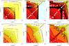 |
Fig. 5 The cosmic variance contributions |


The failure of the normal approximation on small scales has motivated Semboloni et al. (2007) and Sato et al.
(2011b) to develop empirical corrections. Figure 5
shows the covariances resulting from applying the correction factors they proposed for sources
at redshift z = 1 to the cosmic variance part
in the normal approximation3. The estimate based on Semboloni et al.
(2007) overestimates on small scales by a large factor, whereas the
corrections according to Sato et al. (2011b) yield
estimates that underestimate by 20−50%.
Semboloni et al. (2007) and Sato et al. (2011b) do not provide corrections for the cosmic variance
parts or . We thus employ Eqs. (25) and (24) to compute and from the predictions for
. As Fig. 5
shows in comparison to Fig. 4, the estimates based on
Semboloni et al. (2007) fail to reproduce the estimates
from the lensing simulations both quantitatively and qualitatively. On most scales, the
estimate is too large by orders of magnitude. Around the transition scale between the Gaussian
and non-Gaussian regime at 10 arcmin, the estimated covariances show artificially sharp
drops.
The estimates based on Sato et al. (2011b) perform
better. However, they still overpredict the covariances on small scales by a factor of a few,
and underpredict the covariances on large scales. Since the empirical corrections were designed
to yield good estimates of for the range of scales and cosmologies
considered by Semboloni et al. (2007) and Sato et al. (2011b), this indicates that we have used the
corrections outside their range of applicability. For the cosmology and scales considered here,
the log-normal approximation appears to perform better than the empirical corrections.
4.5. Positive-semidefiniteness of the cosmic variance contribution
In the absence of other noise (e.g. ellipticity noise and other sources not considered here),
the cosmic variance part of the cosmic shear covariance represents the full data covariance.
This implies that the actual cosmic variance part of the parameter covariance matrix as well as
its components and are positive-semidefinite regardless of the
statistical properties of the convergence field. Positive-semidefiniteness of the data
covariance is, moreover, an essential requirement for a sound Bayesian parameter inference
employing a quadratic log-likelihood. Thus, a highly desirable property of any approximation to
the cosmic variance contribution is that it yields a positive-semidefinite cosmic variance
part, so that even in cases of high galaxy densities and low ellipticity noise, the full data
covariance remains positive-semidefinite.
In the cases studied here, we encounter a serious problem of the corrections suggested by
Semboloni et al. (2007) and Sato et al. (2011b): both fail to yield positive-semidefinite covariance
parts and . As a consequence, the cosmic variance part of
the data covariance matrix is not positive-semidefinite, but has significantly negative
eigenvalues. This may lead to a non-positive data covariance
matrix Cd, a non-positive parameter covariance
matrix Cπ, and to a breakdown of the
parameter estimation.
Apparently, the empirical corrections do not contain any mechanism ensuring positive-semidefiniteness of the data covariance. Indeed, it seems difficult to devise a valid covariance matrix of correlation functions without strong guidance from, e.g., analytic models.
In contrast, both the normal and the log-normal approximation “should” yield positive-semidefinite covariance matrices by construction, since the resulting matrices are covariance matrices of correlation functions of a (log-)normal field4. Within the simplified log-normal approximation, the cosmic variance part of the covariance matrix is a sum of the cosmic variance part resulting from the normal approximation and another positive-semidefinite matrix, and thus is also expected to be positive-semidefinite. However, due to the employed approximations for finite fields of view and numerical inaccuracies, the normal and (simplified) log-normal approximations may also yield indefinite cosmic variance parts with negative eigenvalues. These negative eigenvalues are found to be essentially consistent with zero, indicating the presence of linear constraints on the data vector (e.g. stemming from the relations (9) and (10)), and of much smaller magnitude than the negative eigenvalues encountered when using the empirical fits. Setting the negative eigenvalues to zero “by hand” does not change the inferred posterior distributions of the parameters significantly for the case of the normal and log-normal approximation, as shown in the following section.
4.6. Error estimates for cosmological parameters from cosmic shear
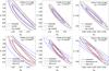 |
Fig. 6 Joint posterior distributions of the mean matter density Ωm and the matter power spectrum normalization σ8 of a flat ΛCDM universe inferred from a cosmic shear survey with ng = 25 arcmin-2 (assuming flat priors for Ωm and σ8, and all other cosmological parameters known). Shown are the 68% (inner) and 95% (outer) confidence contours for a small survey in 5 fields of 2 × 2 deg2 (left panels), a survey in 6 fields of 4 × 4 deg2 (middle panels), and a large survey in a 120 × 120 deg2 field (right panels) obtained when using the covariance matrix measured from our lensing simulations (solid lines), the normal approximation (top, dashed lines), the log-normal approximation (top, dotted lines), the empirical corrections to the normal approximation by Semboloni et al. (2007, bottom, and the corrections by Sato et al. (2011b, bottom. |
To study how the approximations to the cosmic shear covariance affect the inferred accuracy of cosmological-parameter estimation, we consider the scenario that cosmic shear data is used to constrain the parameters Ωm and σ8 of a flat ΛCDM cosmology. To keep the discussion simple, we choose priors that are constant for Ωm ∈ [0.15,0.35] and σ8 ∈ [0.7,1.1] and zero otherwise. Furthermore, we assume the other cosmological parameters known to take the fiducial values: h = 0.73, Ωb = 0.045, and ns = 1.
We assume the cosmic shear correlation functions ξ + (ϑ) and ξ−(ϑ) are measured in 20 logarithmically spaced bins in the range 0.2 arcmin ≤ ϑ ≤ 120 arcmin. The model predictions μ(Ωm,σ8) for the shear correlations are computed using nicaea (Kilbinger et al. 2010). The data vector d containing the measured shear correlations is assumed to coincide with the predicted values for the fiducial cosmology with Ωm = 0.25 and σ8 = 0.9.
As first example, we study the parameter constraints obtained from a small survey with ng = 25 arcmin-2 in 5 fields of 2 × 2 deg2 (i.e. a total area of 20 deg2) similar to the Deep Lens Survey (see, e.g., Kubo et al. 2009). We estimate the inverse covariance matrix directly from the sample covariance of the simulated noisy shear maps using Eq. (32), and combine the estimate with the nicaea predictions to compute the likelihood and the posterior.
In the left panels of Fig. 6, the resulting confidence contours in the (Ωm,σ8)-plane are compared to the contours obtained from the various approximations to the cosmic shear covariance. The normal approximation substantially underestimates the size of the confidence regions, in particular in the direction perpendicular to the major degeneracy. In contrast, the contours based on the log-normal approximation are very similar to the contours based on the measured covariances. The same holds for the simplified log-normal approximation (whose contours are not shown, since they are almost identical to those from the log-normal approximation). Only a slight tilt of the contours based on the (simplified) log-normal approximation against the contours based on the ray-tracing is visible. The corrections proposed by Semboloni et al. (2007) yield confidence regions that are much larger than the regions inferred from the simulations, and are strongly tilted. The confidence regions based on the corrections proposed by Sato et al. (2011b) are noticeably smaller than the regions inferred from the simulations.
As second example, we consider a survey with ng = 25 arcmin-2 in 6 fields of 4 × 4 deg2 (i.e. a total area of 96 deg2) similar to the Canada-France-Hawaii Telescope Wide Synoptic Legacy Survey (Hoekstra et al. 2006). The resulting confidence contours are shown in the middle panels of Fig. 6. As in the first case, the normal approximation underestimates the size of the confidence regions, whereas the (simplified) log-normal approximation yields confidence regions similar to those inferred from our lensing simulations.
As can be seen in the right panels of Fig. 6, the normal approximation substantially underestimates the size of the confidence regions also for very large surveys like the planned Large Synoptic Survey Telescope (LSST) survey (LSST Science Collaborations et al. 2009) or the Euclid survey (Refregier et al. 2010). Even for such large surveys, much cosmological information is contained in the shear correlations on small scales, which are not well described by the normal approximation. The (simplified) log-normal approximation, describing the small scales better, yields confidence regions in much better agreement with the regions inferred from our lensing simulations (using a scaled version of the cosmic covariance measured in the 4 × 4 deg2 fields in combination with analytic expressions for the mixed and ellipticity noise). The contours based on Semboloni et al. (2007) appear much too large and strongly tilted, whereas the contours based on Sato et al. (2011b) appear too small.
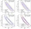 |
Fig. 7 68% (inner) and 95% (outer) confidence contours of the joint posterior distributions of the mean matter density Ωm and the matter power spectrum normalization σ8 of a flat ΛCDM universe inferred from a cosmic shear survey with ng = 70 arcmin-2 in 5 fields of 2 × 2 deg2, obtained using the covariance from our lensing simulations (solid lines), the normal approximation (top, dashed lines), the log-normal approximation (top, dotted lines), the empirical corrections to the normal approximation by Semboloni et al. (2007, bottom, and the corrections by Sato et al. (2011b, bottom. For the left panels, the cosmic covariance parts of the data covariance matrices have be used as given by the approximations. For the right panels, the cosmic variance parts have been modified where needed to ensure positive-semidefiniteness (see text for details). |
In the cases just discussed, both the cosmic variance and the intrinsic ellipticity noise are important sources of error for the inferred parameters. To investigate the case that the cosmic variance is the dominant source of parameter uncertainty, we consider again a survey in 5 fields of 2 × 2 deg2, but with a higher galaxy density ng = 70 arcmin-2. The left panels of Fig. 7 compare confidence contours estimated from the simulations and the contours obtained from the approximations. The normal approximation underestimates the credible parameter regions even more than in the afore discussed cases. The (simplified) log-normal approximation still yields confidence regions comparable in size to those estimated from the simulations, but the shape difference is more apparent (this might become problematic in cases where the compatibility of different cosmological experiments is judged by the overlap of their parameter confidence regions). The confidence regions based on the fit by Semboloni et al. (2007) are of similar size, but strongly tilted.
When using the fits proposed by Sato et al. (2011b), we do not obtain any reasonable confidence contours for the posterior. Both data and parameter covariance matrices are indefinite, and the likelihood features a saddle point at the fiducial parameter values instead of a maximum. The problem can be traced back to the cosmic variance part of the parameter covariance matrix, which is indefinite.
One may approach the problem of negative eigenvalues in the parameter covariance matrix stemming from an indefinite cosmic variance part as follows: using its eigensystem decomposition, the cosmic variance part of the covariance matrix can be specified by an orthogonal set of eigenvectors, which describe the principal directions of scatter in the data vector due to cosmic variance, and the corresponding eigenvalues, which quantify the scatter in these directions. Directions with vanishing scatter indicate linear constraints, which confine all possible data vectors to a lower-dimensional subspace of the full data vector space (in the absence of other sources of scatter). Directions with negative eigenvalues, i.e. “negative scatter”, do not make sense. One may presume, however, these negative eigenvalues stem from numerical inaccuracies in the employed method for computing the cosmic variance, and rather indicate directions with very small positive or vanishing scatter.
To ensure a positive-semidefinite data covariance matrix from the various approximations, we modify the cosmic variance part by replacing any of its negative eigenvalues in its eigensystem decomposition by zero. The resulting confidence contours are shown in the right panels of Fig. 7. There is no visible difference in the contours between the left and right panel for the normal and log-normal approximation, even though their cosmic variance parts have a few negative eigenvalues (which are of tiny magnitude). In contrast, the confidence contours based on the fit by Semboloni et al. (2007) change drastically if the data covariance matrix is modified in the described way. Only after applying the modification, we obtain confidence contours for the correction suggested by Sato et al. (2011b). The parameter confidence regions computed from the modified empirical corrections are much smaller than the confidence regions estimated from the simulations.
5. Summary and discussion
Accurate estimates for the covariance of cosmic shear correlation functions are essential for reliable estimates of the errors on the cosmological parameters inferred from cosmic shear surveys. In this work, we developed two approximations to the cosmic shear covariance based on the statistics of log-normal random fields. We used numerical simulations of cosmic shear surveys to assess the performance of this log-normal and simplified log-normal approximation and to compare them to the widely used normal approximation to the cosmic shear covariance (Schneider et al. 2002a).
We find that the normal approximation to the cosmic shear covariance substantially underestimates the inferred parameter confidence regions, in particular for surveys with small fields of view and large galaxy densities, but also for very large “all sky” surveys (like the proposed Euclid or LSST lensing surveys). The log-normal approximation yields much more realistic confidence regions at the price of slightly more complicated expressions for the cosmic variance contribution to the cosmic shear covariance. In contrast, the simplified log-normal approximation is as simple as the normal approximation, yet appears as accurate as the log-normal approximation. Moreover, the simplified log-normal approximation is simpler than several proposed approximations based on halo models (e.g., Takada & Jain 2009; Pielorz et al. 2010). The simplified log-normal approximation is also more general than approximations based on empirical fits to numerical simulations (Semboloni et al. 2007; Sato et al. 2011b).
A particular advantage of the normal and (simplified) log-normal approximation over the empirical fits suggested by Semboloni et al. (2007) and Sato et al. (2011b) is that the former yield positive-semidefinite data covariance matrices by construction, whereas the latter may fail to do so. A positive-semidefinite data covariance matrix is, however, essential for a sound parameter estimation employing a quadratic log-likelihood.
A disadvantage of the (simplified) log-normal approximation in comparison to the normal approximation is the need for providing a minimum-convergence parameter κ0. The value of this parameter depends on the assumed cosmology as well as the source redshift distribution of the weak-lensing survey. However, computing κ0 does not require more effort than computing the expected shear correlation functions (which are needed in any case). Estimates for κ0 from simulations, for example, require much fewer realisations than estimates for the full cosmic shear covariance.
Because of its comparable simplicity and much better accuracy, one should consider the simplified log-normal approximation in favour of the normal approximation, e.g. for the parameter estimation from current surveys, or for parameter error forecasts for future surveys. For the analysis of observed cosmic shear data from future large and deep surveys, however, better descriptions of the cosmic shear covariance will be required.
In this work, we concentrated on the covariance of the cosmic shear correlations ξ ± and the resulting errors on cosmological parameters. In future work, one should adapt the (simplified) log-normal approximation to derive covariances for other lensing two-point statistics (e.g. the COSEBIs introduced by Schneider et al. 2010). The (simplified) log-normal approximation could also be generalized to provide covariances for tomographic shear surveys. Furthermore, one could consider the approximation of a log-normal convergence field for predictions of higher-order shear correlations and their covariances.
One should also investigate cosmic shear covariances for convergence fields that are more general transformations of normal random random fields (as considered, e.g., by Das & Ostriker 2006; Joachimi et al. 2011). Such work should also take into account the non-Gaussianity and cosmology-dependence of the cosmic shear likelihood (Eifler et al. 2009; Hartlap et al. 2009; Schneider & Hartlap 2009; Sato et al. 2011a; Joachimi & Taylor 2011). Finally, one should investigate further to what extent the matter density field or the convergence field can be described by a transformed normal random field (see, e.g., Neyrinck et al. 2009; Seo et al. 2011; Yu et al. 2011; Joachimi et al. 2011) and what the physical reasons behind the successes and limits of such a description are.
See Appendix C for a detailed discussion of cosmic shear estimators and their noise properties, which also considers a more general estimator with non-uniform weights for the galaxies.
Schneider et al. (2002a) and Joachimi et al. (2008) assume θF ≈ ∞ for simplicity. This is justified for sufficiently large fields, where correlations on scales larger than the field are negligible, and extending the integration boundary of θ3 in Eq. (19) to infinity does not affect the integral significantly. For small survey fields, however, this may lead to an overestimation of the cosmic covariance, which was observed by Sato et al. (2011b) in computer experiments with Gaussian convergence fields.
The corrections by Sato et al. (2011b) assume
explicitly that the normal prediction Eq. (19) is computed with θF = ∞ (as in Schneider et al. 2002a). We thus apply their correction factor to the normal
prediction computed assuming θF = ∞ instead of
 . Moreover we extend the range of the fit
correction F defined in Eq. (B1) to all scales where
F > 1 to avoid discontinuities in the covariance.
. Moreover we extend the range of the fit
correction F defined in Eq. (B1) to all scales where
F > 1 to avoid discontinuities in the covariance.
This certainly holds if the cosmic shear correlations assumed in the computation of the covariances are valid correlation functions of a (log-)normal field, which we checked for our calculations.
Readers interested in a rigorous definition of a normal random field should consult the standard literature on measure theory.
The actual prefactor depends on the particular FFT implementation used.
Acknowledgments
This work was supported by the DFG within the Priority Programme 1177 under the projects SCHN 342/6 and WH 6/3 and the Transregional Collaborative Research Centre TRR 33 “The Dark Universe”.
References
- Anderson, T. W. 2003, an introduction to multivariate statistical analysis, 3rd edn. (Hoboken, New Jersey: John Wiley & Sons, Inc.) [Google Scholar]
- Benjamin, J., Heymans, C., Semboloni, E., et al. 2007, MNRAS, 381, 702 [NASA ADS] [CrossRef] [Google Scholar]
- Blandford, R. D., Saust, A. B., Brainerd, T. G., & Villumsen, J. V. 1991, MNRAS, 251, 600 [NASA ADS] [Google Scholar]
- Brainerd, T. G., Blandford, R. D., & Smail, I. 1996, ApJ, 466, 623 [NASA ADS] [CrossRef] [Google Scholar]
- Coles, P., & Jones, B. 1991, MNRAS, 248, 1 [NASA ADS] [CrossRef] [Google Scholar]
- Cooray, A., & Hu, W. 2001, ApJ, 554, 56 [NASA ADS] [CrossRef] [Google Scholar]
- Crittenden, R. G., Natarajan, P., Pen, U.-L., & Theuns, T. 2002, ApJ, 568, 20 [NASA ADS] [CrossRef] [Google Scholar]
- Das, S., & Ostriker, J. P. 2006, ApJ, 645, 1 [NASA ADS] [CrossRef] [Google Scholar]
- De Lucia, G., & Blaizot, J. 2007, MNRAS, 375, 2 [NASA ADS] [CrossRef] [Google Scholar]
- Eifler, T., Schneider, P., & Hartlap, J. 2009, A&A, 502, 721 [NASA ADS] [CrossRef] [EDP Sciences] [Google Scholar]
- Frigo, M., & Johnson, S. G. 2005, Proc. IEEE, 93, 216 [Google Scholar]
- Fu, L., & Kilbinger, M. 2010, MNRAS, 401, 1264 [NASA ADS] [CrossRef] [Google Scholar]
- Fu, L., Semboloni, E., Hoekstra, H., et al. 2008, A&A, 479, 9 [Google Scholar]
- Hartlap, J., Simon, P., & Schneider, P. 2007, A&A, 464, 399 [NASA ADS] [CrossRef] [EDP Sciences] [Google Scholar]
- Hartlap, J., Schrabback, T., Simon, P., & Schneider, P. 2009, A&A, 504, 689 [NASA ADS] [CrossRef] [EDP Sciences] [Google Scholar]
- Hilbert, S., White, S. D. M., Hartlap, J., & Schneider, P. 2007, MNRAS, 382, 121 [NASA ADS] [CrossRef] [Google Scholar]
- Hilbert, S., White, S. D. M., Hartlap, J., & Schneider, P. 2008, MNRAS, 386, 1845 [NASA ADS] [CrossRef] [Google Scholar]
- Hilbert, S., Hartlap, J., White, S. D. M., & Schneider, P. 2009, A&A, 499, 31 [NASA ADS] [CrossRef] [EDP Sciences] [Google Scholar]
- Hoekstra, H., Mellier, Y., van Waerbeke, L., et al. 2006, ApJ, 647, 116 [NASA ADS] [CrossRef] [Google Scholar]
- Hubble, E. 1934, ApJ, 79, 8 [NASA ADS] [CrossRef] [Google Scholar]
- Huterer, D. 2010, General Relativity and Gravitation, 42, 2177 [NASA ADS] [CrossRef] [Google Scholar]
- Joachimi, B., & Taylor, A. N. 2011, MNRAS, 416, 1010 [NASA ADS] [CrossRef] [Google Scholar]
- Joachimi, B., Schneider, P., & Eifler, T. 2008, A&A, 477, 43 [NASA ADS] [CrossRef] [EDP Sciences] [Google Scholar]
- Joachimi, B., Taylor, A. N., & Kiessling, A. 2011, MNRAS, 1390 [Google Scholar]
- Kainulainen, K., & Marra, V. 2011, Phys. Rev. D, 83, 023009 [NASA ADS] [CrossRef] [Google Scholar]
- Kaiser, N. 1992, ApJ, 388, 272 [NASA ADS] [CrossRef] [Google Scholar]
- Kaiser, N. 1995, ApJ, 439, L1 [NASA ADS] [CrossRef] [Google Scholar]
- Kayo, I., Taruya, A., & Suto, Y. 2001, ApJ, 561, 22 [NASA ADS] [CrossRef] [Google Scholar]
- Kilbinger, M., Benabed, K., McCracken, H. J., & Fu, L. 2010, NumerIcal Cosmology And lEnsing cAlculations (NICAEA) version 2.3, http://www2.iap.fr/users/kilbinge/nicaea/ [Google Scholar]
- Kofman, L., Bertschinger, E., Gelb, J. M., Nusser, A., & Dekel, A. 1994, ApJ, 420, 44 [NASA ADS] [CrossRef] [Google Scholar]
- Krause, E., & Hirata, C. M. 2010, A&A, 523, A28 [NASA ADS] [CrossRef] [EDP Sciences] [Google Scholar]
- Kubo, J. M., Khiabanian, H., Dell’ Antonio, I. P., Wittman, D., & Tyson, J. A. 2009, ApJ, 702, 980 [NASA ADS] [CrossRef] [Google Scholar]
- LSST Science Collaborations, Abell, P. A., Allison, J., et al. 2009 [arXiv:0912.0201] [Google Scholar]
- Martin, S., Schneider, P., & Simon, P. 2011, A&A, submitted [arXiv:1109.0944] [Google Scholar]
- Massey, R., Rhodes, J., Leauthaud, A., et al. 2007, ApJS, 172, 239 [NASA ADS] [CrossRef] [MathSciNet] [Google Scholar]
- Mould, J., Blandford, R., Villumsen, J., et al. 1994, MNRAS, 271, 31 [NASA ADS] [Google Scholar]
- Neyrinck, M. C., Szapudi, I., & Szalay, A. S. 2009, ApJ, 698, L90 [NASA ADS] [CrossRef] [Google Scholar]
- Pielorz, J., Rödiger, J., Tereno, I., & Schneider, P. 2010, A&A, 514, A79 [NASA ADS] [CrossRef] [EDP Sciences] [Google Scholar]
- Refregier, A., Amara, A., Kitching, T. D., et al. 2010 [arXiv:1001.0061] [Google Scholar]
- Sato, M., Hamana, T., Takahashi, R., et al. 2009, ApJ, 701, 945 [NASA ADS] [CrossRef] [Google Scholar]
- Sato, M., Ichiki, K., & Takeuchi, T. T. 2011a, Phys. Rev. D, 83, 023501 [NASA ADS] [CrossRef] [Google Scholar]
- Sato, M., Takada, M., Hamana, T., & Matsubara, T. 2011b, ApJ, 734, 76 [NASA ADS] [CrossRef] [Google Scholar]
- Schneider, P., & Hartlap, J. 2009, A&A, 504, 705 [NASA ADS] [CrossRef] [EDP Sciences] [Google Scholar]
- Schneider, P., & Kilbinger, M. 2007, A&A, 462, 841 [NASA ADS] [CrossRef] [EDP Sciences] [Google Scholar]
- Schneider, P., van Waerbeke, L., Jain, B., & Kruse, G. 1998, MNRAS, 296, 873 [NASA ADS] [CrossRef] [Google Scholar]
- Schneider, P., van Waerbeke, L., Kilbinger, M., & Mellier, Y. 2002a, A&A, 396, 1 [NASA ADS] [CrossRef] [EDP Sciences] [Google Scholar]
- Schneider, P., van Waerbeke, L., & Mellier, Y. 2002b, A&A, 389, 729 [NASA ADS] [CrossRef] [EDP Sciences] [Google Scholar]
- Schneider, P., Kochanek, C., & Wambsganss, J. 2006, Gravitational Lensing: Strong, Weak and Micro, Saas-Fee Advanced Course 33 (Berlin: Springer) [Google Scholar]
- Schneider, P., Eifler, T., & Krause, E. 2010, A&A, 520, A116 [NASA ADS] [CrossRef] [EDP Sciences] [Google Scholar]
- Schrabback, T., Hartlap, J., Joachimi, B., et al. 2010, A&A, 516, A63 [NASA ADS] [CrossRef] [EDP Sciences] [Google Scholar]
- Scoccimarro, R., Zaldarriaga, M., & Hui, L. 1999, ApJ, 527, 1 [NASA ADS] [CrossRef] [Google Scholar]
- Semboloni, E., Mellier, Y., van Waerbeke, L., et al. 2006, A&A, 452, 51 [NASA ADS] [CrossRef] [EDP Sciences] [Google Scholar]
- Semboloni, E., van Waerbeke, L., Heymans, C., et al. 2007, MNRAS, 375, L6 [NASA ADS] [CrossRef] [Google Scholar]
- Semboloni, E., Schrabback, T., van Waerbeke, L., et al. 2011, MNRAS, 410, 143 [NASA ADS] [CrossRef] [Google Scholar]
- Seo, H.-J., Sato, M., Dodelson, S., Jain, B., & Takada, M. 2011, ApJ, 729, L11 [NASA ADS] [CrossRef] [Google Scholar]
- Springel, V. 2005, MNRAS, 364, 1105 [NASA ADS] [CrossRef] [Google Scholar]
- Springel, V., White, S. D. M., Jenkins, A., et al. 2005, Nature, 435, 629 [NASA ADS] [CrossRef] [PubMed] [Google Scholar]
- Takada, M., & Jain, B. 2009, MNRAS, 395, 2065 [NASA ADS] [CrossRef] [Google Scholar]
- Takahashi, R., Oguri, M., Sato, M., & Hamana, T. 2011, ApJ, 742, 15 [NASA ADS] [CrossRef] [Google Scholar]
- Taruya, A., Takada, M., Hamana, T., Kayo, I., & Futamase, T. 2002, ApJ, 571, 638 [NASA ADS] [CrossRef] [Google Scholar]
- Vale, C., & White, M. 2003, ApJ, 592, 699 [NASA ADS] [CrossRef] [Google Scholar]
- Van Waerbeke, L., Hamana, T., Scoccimarro, R., Colombi, S., & Bernardeau, F. 2001, MNRAS, 322, 918 [NASA ADS] [CrossRef] [Google Scholar]
- Yu, Y., Zhang, P., Lin, W., Cui, W., & Fry, J. N. 2011, Phys. Rev. D, 84, 023523 [NASA ADS] [CrossRef] [Google Scholar]
Appendix A: Normal random fields
Consider a non-degenerate homogeneous and isotropic normal random field n in
D dimensions5. This implies that the
probability density function (pdf) of the field values
n = n(x) at any single point
x ∈ RD is given by ![Mathematical equation: \appendix \setcounter{section}{1} \begin{equation} p_n(n;\mu,\sigma) = \frac{1}{\sqrt{2\pi} \sigma}\exp\left[-\frac{\left(n - \mu\right)^2}{2\sigma^2}\right], \label{eq:normal_pdf} \end{equation}](/articles/aa/full_html/2011/12/aa17294-11/aa17294-11-eq211.png) (A.1)where μ and
σ2 denote the position-independent mean and variance of the random
variable n(x). Moreover, the joint pdf of the
field values
n = (n1,...,nN)t = (n(x1),...,n(xN))t
at a set of N mutually distinct points
x1,...,xN
is given by the pdf of a non-degenerate multivariate normal distribution:
(A.1)where μ and
σ2 denote the position-independent mean and variance of the random
variable n(x). Moreover, the joint pdf of the
field values
n = (n1,...,nN)t = (n(x1),...,n(xN))t
at a set of N mutually distinct points
x1,...,xN
is given by the pdf of a non-degenerate multivariate normal distribution: ![Mathematical equation: \appendix \setcounter{section}{1} \begin{equation} p_{\vect{n}} \big(\vect{n};\vect{\mu},\matrb{\Sigma}\big) = \frac{1}{(2\pi)^{N/2}\sqrt{\det\matrb{\Sigma}}} \exp\left[-\frac{1}{2}\transposed{(\vect{n} - \vect{\mu})} \matrb{\Sigma}^{-1}(\vect{n} - \vect{\mu}) \right]. \label{eq:normal_field_multivariate_pdf} \end{equation}](/articles/aa/full_html/2011/12/aa17294-11/aa17294-11-eq216.png) (A.2)Here,
μ = ⟨n⟩ = μ1
with
1 = (1,...,1)t
in accordance with the requirement of homogeneity. The covariance
matrix Σ is a positive-definite real symmetric matrix, whose
elements Σij are given by the two-point
correlations ξn,ij of the
field n. Since the field is homogeneous and isotropic, the two-point
correlation ξn,ij
of field values at points xi
and xj depends only on their
separation, i.e.
(A.2)Here,
μ = ⟨n⟩ = μ1
with
1 = (1,...,1)t
in accordance with the requirement of homogeneity. The covariance
matrix Σ is a positive-definite real symmetric matrix, whose
elements Σij are given by the two-point
correlations ξn,ij of the
field n. Since the field is homogeneous and isotropic, the two-point
correlation ξn,ij
of field values at points xi
and xj depends only on their
separation, i.e.  (A.3)where
ξn(ϑ) denotes the correlation
function of the field n at separation ϑ. In particular, the
diagonal elements of Σ are given by the
variance σ2,
i.e. Σii = ξ(0) = σ2.
(A.3)where
ξn(ϑ) denotes the correlation
function of the field n at separation ϑ. In particular, the
diagonal elements of Σ are given by the
variance σ2,
i.e. Σii = ξ(0) = σ2.
Using the joint pdf (A.2), the expectation
value ⟨f(n)⟩ of a
function f(n) depending on the field values
n = (n(x1),...,n(xN))t
at N positions
x1,...,xN
can be written as ![Mathematical equation: \appendix \setcounter{section}{1} \begin{equation} \EV{f(\vect{n})} = \int_{\R^N}\!\!\diff[N]{\vect{n}}\, \frac{1}{(2\pi)^{N/2}\sqrt{\det\matrb{\Sigma}}} \exp\left[ -\frac{1}{2}\transposed{(\vect{n} - \vect{\mu})} \matrb{\Sigma}^{-1}(\vect{n} - \vect{\mu})\right] f(\vect{n}). \end{equation}](/articles/aa/full_html/2011/12/aa17294-11/aa17294-11-eq231.png) (A.4)The moment-generating function for the field values
n = (n1,...,nN)t
at N mutually distinct points
x1,...,xN
is defined as the map
(A.4)The moment-generating function for the field values
n = (n1,...,nN)t
at N mutually distinct points
x1,...,xN
is defined as the map  (A.5)For a normal random field,
![Mathematical equation: \appendix \setcounter{section}{1} \begin{eqnarray} M_{\vect{n}}( \vect{t} ) = \EV{\exp(\transposed{\vect{t}} \vect{n})} &= & \int_{\R^N}\!\!\diff[N]{\vect{n}}\, \frac{1}{(2\pi)^{N/2}\sqrt{\det\matrb{\Sigma}}} \exp\left[ -\frac{1}{2}\transposed{(\vect{n} - \vect{\mu})} \matrb{\Sigma}^{-1}(\vect{n} - \vect{\mu}) + \transposed{\vect{t}} \vect{n} \right] \nonumber\\ &=& \int_{\R^N}\!\!\diff[N]{\vect{n}}\, \frac{1}{(2\pi)^{N/2}\sqrt{\det\matrb{\Sigma}}} \exp\left[ -\frac{1}{2}\transposed{\left(\vect{n} - \vect{\mu} - \matrb{\Sigma} \vect{t} \right)} \matrb{\Sigma}^{-1} \left(\vect{n} - \vect{\mu} - \matrb{\Sigma} \vect{t} \right) + \transposed{\vect{t}} \vect{\mu} +\frac{1}{2} \transposed{\vect{t}} \matrb{\Sigma} \vect{t} \right] = \exp\left[\transposed{\vect{t}} \vect{\mu} + \frac{1}{2} \transposed{\vect{t}} \matrb{\Sigma} \vect{t} \right]. \end{eqnarray}](/articles/aa/full_html/2011/12/aa17294-11/aa17294-11-eq234.png) (A.6)Using
Mn, the
m1...mN-point
correlation function composed of powers
m1,...,mN
of the field values
n1,...,nN
can be computed by
(A.6)Using
Mn, the
m1...mN-point
correlation function composed of powers
m1,...,mN
of the field values
n1,...,nN
can be computed by ![Mathematical equation: \appendix \setcounter{section}{1} \begin{eqnarray} \EV{n_1^{m_1}\ldots n_N^{m_N}} &= \left. \frac{\partial^{m_1\cdots m_N} M_{\vect{n}}(\vect{t})}{\partial t_1^{m_1}\ldots\partial t_N^{m_N}}\right|_{\vect{t}=\vect{0}} = \left. \frac{\partial^{m_1\cdots m_N}}{\partial t_1^{m_1} \cdots \partial t_N^{m_N}} \exp\left[\transposed{\vect{t}}\vect{\mu} + \frac{1}{2} \transposed{\vect{t}} \matrb{\Sigma} \vect{t} \right] \right|_{\vect{t}=\vect{0}}. \end{eqnarray}](/articles/aa/full_html/2011/12/aa17294-11/aa17294-11-eq239.png) (A.7)For example,
(A.7)For example,  In a similar manner, one can compute expectation
values for products of powers
k1,...,kN
of exponentiated field
values exp(n1),...,exp(nN):
In a similar manner, one can compute expectation
values for products of powers
k1,...,kN
of exponentiated field
values exp(n1),...,exp(nN):
![Mathematical equation: \appendix \setcounter{section}{1} \begin{eqnarray} \label{eq:ev_log_prod} \EV{\exp(n_1)^{k_1}\cdots \exp(n_N)^{k_N}} &=& \EV{\exp\left( \transposed{\vect{k}}\vect{n} \right)} = \exp\left[\transposed{\vect{k}}\vect{\mu} + \frac{1}{2} \transposed{\vect{k}} \matrb{\Sigma} \vect{k} \right] = \exp\bigg[\sum_{i=1}^{N}\left(k_i \mu + k_i^2 \frac{\sigma^2}{2}\right) + \sum_{i<j} k_i k_j \xi_n\big(|\vect{x}_i - \vect{x}_j|\big) \bigg] \nonumber\\&& = \lambda^{\transposed{\vect{k}}\vect{1}} \eta_0^{\transposed{\vect{k}}(\vect{k}-\vect{1})/2} \prod_{i<j} \eta_{ij}^{k_i k_j}, \end{eqnarray}](/articles/aa/full_html/2011/12/aa17294-11/aa17294-11-eq243.png) (A.11)where
λ = exp(μ + σ2/2),
k = (k1,...,kN)t,
(A.11)where
λ = exp(μ + σ2/2),
k = (k1,...,kN)t,
 , and
ηij = η(| xi − xj|)
with
η(r) = exp[ξn(r)].
In particular,
, and
ηij = η(| xi − xj|)
with
η(r) = exp[ξn(r)].
In particular, 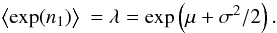 (A.12)
Appendix B: Zero-mean shifted log-normal random fields
A zero-mean shifted log-normal homogeneous and isotropic random field z can
be defined via ![Mathematical equation: \appendix \setcounter{section}{2} \begin{equation} z : \R^D \to \R : \vect{x} \mapsto z(\vect{x}) = \exp\big[n(\vect{x})\big] - \lambda, \end{equation}](/articles/aa/full_html/2011/12/aa17294-11/aa17294-11-eq250.png) (B.1)where n is a homogeneous and
isotropic normal field with mean μ and
variance σ2, and the shift
λ = exp(μ + σ2/2)
to ensure vanishing mean for z. The one-point distribution of the random
field z reads
(B.1)where n is a homogeneous and
isotropic normal field with mean μ and
variance σ2, and the shift
λ = exp(μ + σ2/2)
to ensure vanishing mean for z. The one-point distribution of the random
field z reads ![Mathematical equation: \appendix \setcounter{section}{2} \begin{equation} p_z(z; \lambda, \sigma) = \begin{cases} \dfrac{1}{\sqrt{2\pi}(z + \lambda)\sigma} \exp\Biggl\{-\dfrac{\bigl[\ln\left(z / \lambda + 1\right) + \sigma^2/2 \bigr]^2}{2\sigma^2}\Biggr\} & {\rm for }\;\; z > - \lambda {\rm , ~~and}\\ 0 & {\rm otherwise.} \end{cases} \label{eq:zero_mean_shifted_log_normal_pdf} \end{equation}](/articles/aa/full_html/2011/12/aa17294-11/aa17294-11-eq251.png) (B.2)The negative of the shift λ marks
the lower limit for possible values for z.
(B.2)The negative of the shift λ marks
the lower limit for possible values for z.
The N-point correlation of z can be deduced from the
two-point correlation of the underlying normal field n as follows. First note
that an
m1...mN-point
correlation function of z composed of powers
m1,...,mN
of the field values
z1,...,zN
at N mutually distinct points
x1,...,xN
can be written as: ![Mathematical equation: \appendix \setcounter{section}{2} \begin{eqnarray} \label{eq:shifted_log_prod_to_sum_of_log_prod} \EV{z_1^{m_1}\ldots z_N^{m_N}} = \EV{\prod_{i=1}^{N} \left[\exp(n_i) - \lambda\right]^{m_i}} = \EV{\prod_{i=1}^{N} \sum_{k_i = 0}^{m_i} \binom{m_i}{k_i} (-\lambda)^{m_i - k_i} \exp(n_i)^{k_i}} = \sum_{k_1 = 0}^{m_1} \binom{m_1}{k_1} \ldots\sum_{k_N = 0}^{m_N} \binom{m_N}{k_N} (-\lambda)^{ \transposed{(\vect{m} - \vect{k})}\vect{1}} \EV{\exp\bigl(\transposed{\vect{k}} \vect{n}\bigr)}, \end{eqnarray}](/articles/aa/full_html/2011/12/aa17294-11/aa17294-11-eq254.png) (B.3)where
k = (k1,...,kN)t
and
m = (m1,...,mN)t.
Combining the results of Eqs. (B.3) and (A.11), one obtains
(B.3)where
k = (k1,...,kN)t
and
m = (m1,...,mN)t.
Combining the results of Eqs. (B.3) and (A.11), one obtains
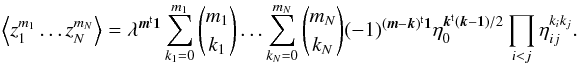 (B.4)For example,
 ![Mathematical equation: \appendix \setcounter{section}{2} \begin{eqnarray} \label{eq:zero_shifted_log_normal_2p_correlation} &&\EV{z_1 z_2} = \lambda^2 \bigl[\eta_{12} - 1 \bigr] = \lambda^2 \bigl\{\exp\big[\xi_n\big(|\vect{x}_i - \vect{x}_j|\big)\big] - 1 \bigr\} = \xi_z\big(|\vect{x}_i - \vect{x}_j|\big), \end{eqnarray}](/articles/aa/full_html/2011/12/aa17294-11/aa17294-11-eq258.png) (B.5)
(B.5)![Mathematical equation: \appendix \setcounter{section}{2} \begin{eqnarray} &&\EV{z_1 z_2 z_3} = \lambda^3 \bigl[ \eta_{12}\eta_{13}\eta_{23} - \eta_{12} - \eta_{13} - \eta_{23} + 2 \bigr] {\rm , and} \end{eqnarray}](/articles/aa/full_html/2011/12/aa17294-11/aa17294-11-eq259.png) (B.6)
(B.6)![Mathematical equation: \appendix \setcounter{section}{2} \begin{eqnarray} \label{eq:zero_shifted_log_normal_4p_correlation} &&\EV{z_1 z_2 z_3 z_4} = \lambda^4 \bigl[ \eta_{12}\eta_{13}\eta_{14} \eta_{23} \eta_{24} \eta_{34} - \eta_{12}\eta_{13}\eta_{23} - \eta_{12}\eta_{14}\eta_{24} - \eta_{13}\eta_{14}\eta_{34} - \eta_{23}\eta_{24}\eta_{34} + \eta_{12} + \eta_{13} + \eta_{14} + \eta_{23} + \eta_{24} + \eta_{34} - 3 \bigr]. \end{eqnarray}](/articles/aa/full_html/2011/12/aa17294-11/aa17294-11-eq260.png) (B.7)From Eq. (B.5) follows that the correlation functions
ξz(r) and
ξn(r) are related via
(B.7)From Eq. (B.5) follows that the correlation functions
ξz(r) and
ξn(r) are related via
![Mathematical equation: \appendix \setcounter{section}{2} \begin{equation} \xi_z(r) = \lambda^2 \bigl\{\exp\big[\xi_n(r)\big] - 1 \bigr\} \qquad\Leftrightarrow\qquad \xi_n(r) = \ln\big[\lambda^{-2} \xi_z(r) + 1\big]. \end{equation}](/articles/aa/full_html/2011/12/aa17294-11/aa17294-11-eq263.png) (B.8)The correlation function
ξz(r) and the function
η(r) = exp[ξn(r)]
are related via
(B.8)The correlation function
ξz(r) and the function
η(r) = exp[ξn(r)]
are related via ![Mathematical equation: \appendix \setcounter{section}{2} \begin{equation} \xi_z(r) = \lambda^2 \bigl[\eta(r) - 1 \bigr] \qquad\Leftrightarrow\qquad \eta(r) = \lambda^{-2}\xi_z(r) + 1. \label{eq:xi_z_of_r_from_eta_of_r} \end{equation}](/articles/aa/full_html/2011/12/aa17294-11/aa17294-11-eq264.png) (B.9)Using these relations, one obtains, e.g.
(B.9)Using these relations, one obtains, e.g.
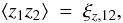 (B.10)
![Mathematical equation: \appendix \setcounter{section}{2} \begin{eqnarray} \label{eq:zero_shifted_log_normal_3p_correlation_of_xi} \EV{z_1 z_2 z_3} &=& \lambda^{-1}\left[\xi_{z,12}\xi_{z,13} + \xi_{z,12}\xi_{z,23} + \xi_{z,13} \xi_{z,23}\right] + \lambda^{-3} \xi_{z,12} \xi_{z,13} \xi_{z,23} {\rm , and} \end{eqnarray}](/articles/aa/full_html/2011/12/aa17294-11/aa17294-11-eq266.png) (B.11)
(B.11)![Mathematical equation: \appendix \setcounter{section}{2} \begin{eqnarray} \label{eq:zero_shifted_log_normal_4p_correlation_of_xi} \EV{z_1 z_2 z_3 z_4} &=& \xi_{z,12}\xi_{z,34} + \xi_{z,13}\xi_{z,24} + \xi_{z,14} \xi_{z,23} + \lambda^{-2}\left[\xi_{z,12}\xi_{z,13}\xi_{z,14} + \xi_{z,12}\xi_{z,13}\xi_{z,24} + \xi_{z,12}\xi_{z,13}\xi_{z,34} + \ldots\right] \nonumber\\ &&\qquad\qquad\quad + \lambda^{-4}\left[\xi_{z,12}\xi_{z,13}\xi_{z,14} \xi_{z,23} + \ldots\right] + \lambda^{-6}\left[\xi_{z,12}\xi_{z,13}\xi_{z,14} \xi_{z,23} \xi_{z,24} + \ldots\right] + \lambda^{-8}\xi_{z,12}\xi_{z,13}\xi_{z,14}\xi_{z,23}\xi_{z,24}\xi_{z,34}. \end{eqnarray}](/articles/aa/full_html/2011/12/aa17294-11/aa17294-11-eq267.png) (B.12)
(B.12)
Appendix C: Statistical properties of the shear-correlation estimator
In this section, we give a detailed discussion of approximations to the noise properties of the commonly used shear-correlation estimators (13). The discussion loosely follows the real-space approach of Schneider et al. (2002a). In contrast to previous works, we do not restrict the discussion to Gaussian shear fields. Instead, we first derive expressions for the covariance of the shear-correlation estimators for the case of a general convergence field, and then discuss the special cases of normal and zero-mean shifted log-normal convergence fields.
C.1. Basic assumptions and definitions
To obtain analytical expressions for the statistical properties of the shear-correlation estimator, we consider an ensemble of weak-lensing surveys with Ng galaxies in a rectangular field F with area AF, which implies a galaxy number density ng = Ng/AF. To keep the computations simple, we make the following additional assumptions:
-
The number of galaxies is large, i.e. Ng ≫ 1.
-
Periodic boundary conditions are assumed for the distortion field (i.e. we neglect effects of field boundaries and distortions caused by structures outside the survey area).
-
The shear field γ is generated by a convergence field κ in the survey field (i.e. we neglect B-mode shear).
-
The convergence field κ is a realisation of a statistically homogeneous and isotropic random field (we ignore that the assumption of statistical isotropy is in conflict with the assumption of periodic boundary conditions).
-
The galaxy positions θ(1),...,θ(N) are uniformly and independently distributed in the survey field (i.e. we neglect correlations between the galaxy positions).
-
The galaxy redshifts z(1),...,z(N) are identically and independently distributed according to a redshift distribution pz(z) (i.e. we neglect correlations between the galaxy redshifts).
-
The observed image ellipticity
 of each galaxy is a sum of its intrinsic ellipticity
ϵ(i) and the shear
γ(i) = γ(θ(i),z(i))
at the galaxy’s position θ(i) and
redshift z(i).
of each galaxy is a sum of its intrinsic ellipticity
ϵ(i) and the shear
γ(i) = γ(θ(i),z(i))
at the galaxy’s position θ(i) and
redshift z(i). -
The intrinsic ellipticities ϵ(1),...,ϵ(N) are identically and independently distributed and are not correlated with the shear field (i.e. we neglect intrinsic alignments). The joint distribution of the two components
 and
and  of each intrinsic ellipticity
ϵ(i) is isotropic with vanishing mean and
variance
of each intrinsic ellipticity
ϵ(i) is isotropic with vanishing mean and
variance  per dimension (i.e. we neglect complications
due to non-isotropic intrinsic ellipticity distributions caused, e.g, by insufficient PSF
corrections).
per dimension (i.e. we neglect complications
due to non-isotropic intrinsic ellipticity distributions caused, e.g, by insufficient PSF
corrections).
The Fourier transform  of a real function
f(θ) on the survey field is defined by the
relations:
of a real function
f(θ) on the survey field is defined by the
relations: ![Mathematical equation: \appendix \setcounter{section}{3} \begin{eqnarray} \ft{f}(\vell) &=& \frac{1}{\AFOV}\int_{\FOV}\idiff[2]{\vtheta} \ee^{-\ii \vell \cdot \vtheta} f(\vtheta) \qquad\Leftrightarrow\qquad f(\vtheta) = \sum_{\vell} \ee^{\ii \vell \cdot \vtheta} \ft{f}(\vell). \end{eqnarray}](/articles/aa/full_html/2011/12/aa17294-11/aa17294-11-eq279.png) (C.1)Expectation values
(C.1)Expectation values
 of observables
  are obtained by computing the following (formal) average:
 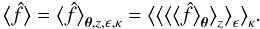 (C.2)Here,
  denotes the ensemble average over the realisations of the convergence field,
 denotes the average over the intrinsic ellipticities,
![Mathematical equation: \appendix \setcounter{section}{3} \begin{equation} \bEV{\est{f}}_{\zgal} = \int\idiff[]{\zgal^{(1)}} p_z\bigl(\zgal^{(1)}\bigr) \ldots \int\diff[]{\zgal^{(\Ngal)}}p_z\bigl(\zgal^{(\Ngal)}\bigr) \est{f}\bigl(\thetagal^{(1)},\ldots\bigr) \end{equation}](/articles/aa/full_html/2011/12/aa17294-11/aa17294-11-eq285.png) (C.3)denotes the average over the galaxy redshifts, and
(C.3)denotes the average over the galaxy redshifts, and
![Mathematical equation: \appendix \setcounter{section}{3} \begin{equation} \bEV{\est{f}}_{\thetagal} = \frac{1}{\AFOV^{\Ngal}}\int_{\FOV}\idiff[2]{\thetagal^{(1)}} \cdots \int_{\FOV}\idiff[2]{\thetagal^{(\Ngal)}} \est{f}\bigl(\thetagal^{(1)},\ldots\bigr) \end{equation}](/articles/aa/full_html/2011/12/aa17294-11/aa17294-11-eq286.png) (C.4)denotes the ensemble average over the galaxy
positions. We assume that the order of the averages does not matter for all observables of
interest.
(C.4)denotes the ensemble average over the galaxy
positions. We assume that the order of the averages does not matter for all observables of
interest.
The tangential component
γt(θ,ϑ,z)
and cross component
γ × (θ,ϑ,z)
of the shear γ(θ,z) at
position θ and redshift z with respect to the
direction ϑ are defined by (e.g. Schneider et al. 2002b)  (C.5)where
ϕ(ϑ) denotes the polar angle of the
vector ϑ.
(C.5)where
ϕ(ϑ) denotes the polar angle of the
vector ϑ.
We denote the tangential and cross component of the shear
γ(i) = γ(θ(i),z(i))
at position θ(i) and redshift
z(i) of a galaxy i with respect
to the direction
ϕ(i,j) = ϕ(θ(j) − θ(i))
towards a galaxy j at position
θ(j) by
 (C.6)Similar definitions are made for the tangential and
cross component of the intrinsic and observed image ellipticity:
(C.6)Similar definitions are made for the tangential and
cross component of the intrinsic and observed image ellipticity:
 (C.7)
(C.7) (C.8)Furthermore, we define the source-redshift averaged
convergence κ(θ) and shear
γ(θ) as in Eqs. (3) and (4). From the assumption that the shear field is generated by the convergence field
follows that the convergence and the Cartesian shear components are related in Fourier
space by:
(C.8)Furthermore, we define the source-redshift averaged
convergence κ(θ) and shear
γ(θ) as in Eqs. (3) and (4). From the assumption that the shear field is generated by the convergence field
follows that the convergence and the Cartesian shear components are related in Fourier
space by: ![Mathematical equation: \appendix \setcounter{section}{3} \begin{equation} \ft{\gamma}_1(\vell) = \cos\bigl[2\varphi(\vell)\bigr] \ft{\kappa}(\vell) \qquad{\rm and}\qquad \ft{\gamma}_2(\vell) = \sin\bigl[2\varphi(\vell)\bigr] \ft{\kappa}(\vell). \label{eq:relation_ft_kappa_gamma} \end{equation}](/articles/aa/full_html/2011/12/aa17294-11/aa17294-11-eq298.png) (C.9)We define the tangential and cross components of
the effective shear as in Eqs. (5) and (6). With these definitions,
(C.9)We define the tangential and cross components of
the effective shear as in Eqs. (5) and (6). With these definitions,  (C.10)
![Mathematical equation: \appendix \setcounter{section}{3} \begin{eqnarray} \label{eq:gtgt_m_gxgx_to_cartesian} \gammat(\vtheta,\vvartheta)\gammat(\vtheta + \vvartheta,\vvartheta) - \gammax(\vtheta,\vvartheta)\gammax(\vtheta + \vvartheta,\vvartheta) &=& \cos\bigl[4\varphi(\vvartheta)\bigr]\bigl[ \gamma_1(\vtheta)\gamma_1(\vtheta + \vvartheta) - \gamma_2(\vtheta)\gamma_2(\vtheta + \vvartheta) \bigr] \nonumber\\ &&\quad + \sin\bigl[4\varphi(\vvartheta)\bigr]\bigl[ \gamma_1(\vtheta)\gamma_2(\vtheta + \vvartheta) + \gamma_2(\vtheta)\gamma_1(\vtheta + \vvartheta) \bigr]. \end{eqnarray}](/articles/aa/full_html/2011/12/aa17294-11/aa17294-11-eq300.png) (C.11)
(C.11)
C.2. Correlation functions and their relations
There exist well-known relations between the two-point correlations of the convergence and the shear, e.g. Eqs. (9) and (10). We wish to derive similar relations between the four-point correlations of the convergence and the four-point correlations of the shear, which appear in the covariance of the cosmic shear estimators (13). Achieving this task for general convergence fields requires relations between the convergence and the shear that hold not only for the ensemble mean, but for every realisation of the convergence field.
For every realisation, we define “empirical” correlations based on spatial averages:
![Mathematical equation: \appendix \setcounter{section}{3} \begin{equation} \spavxi_{\kappa} (\vtheta) = \frac{1}{\AFOV} \int_{\FOV} \idiff[2]{\vtheta'} \kappa(\vtheta') \kappa(\vtheta' +\vtheta) \qquad{\rm and}\qquad \spavxi_{\pm} (\vtheta) = \frac{1}{\AFOV} \int_{\FOV} \idiff[2]{\vtheta'} \left[\gammat(\vtheta',\vtheta) \gammat(\vtheta' +\vtheta,\vtheta) \pm \gammax(\vtheta',\vtheta) \gammax(\vtheta' + \vtheta,\vtheta) \right]. \label{eq:df_empirical_correlations} \end{equation}](/articles/aa/full_html/2011/12/aa17294-11/aa17294-11-eq301.png) (C.12)From the convolution theorem and the relations
(C.9)−(C.11) follows that for every realisation,
(C.12)From the convolution theorem and the relations
(C.9)−(C.11) follows that for every realisation,
![Mathematical equation: \appendix \setcounter{section}{3} \begin{eqnarray} \spavxi_{+} (\vtheta) &=& \frac{1}{\AFOV} \int_{\FOV} \idiff[2]{\vtheta'} \left[\gamma_1(\vtheta') \gamma_1(\vtheta' +\vtheta) + \gamma_2(\vtheta') \gamma_2(\vtheta' + \vtheta) \right] = \sum_{\vell} \ee^{\ii \vell \cdot \vtheta} \left\{\cos\bigl[2\varphi(\vell)\bigr]^2 + \sin\bigl[2\varphi(\vell)\bigr]^2 \right\} \ft{\kappa}^*(\vell) \ft{\kappa}(\vell) = \sum_{\vell} \ee^{\ii \vell \cdot \vtheta} \ft{\kappa}^*(\vell) \ft{\kappa}(\vell) \nonumber\\[3mm] &=& \spavxi_{\kappa}(\vtheta) {\rm , and} \\[3mm] \spavxi_{-} (\vtheta) &= & \frac{1}{\AFOV} \int_{\FOV} \idiff[2]{\vtheta'} \Bigl\{ \cos\bigl[4 \varphi(\vtheta)\bigr] \left[\gamma_1(\vtheta') \gamma_1(\vtheta' +\vtheta) - \gamma_2(\vtheta') \gamma_2(\vtheta' + \vtheta) \right] + \sin\bigl[4 \varphi(\vtheta)\bigr] \left[\gamma_1(\vtheta') \gamma_2(\vtheta' +\vtheta) - \gamma_2(\vtheta') \gamma_1(\vtheta' + \vtheta) \right] \Bigr\} \nonumber\\[3mm] &=& \sum_{\vell} \ee^{\ii \vell \cdot \vtheta} \left\{\cos\bigl[4 \varphi(\vtheta)\bigr]\cos\bigl[2\varphi(\vell)\bigr]^2 - \cos\bigl[4 \varphi(\vtheta)\bigr]\sin\bigl[2\varphi(\vell)\bigr]^2 + 2 \sin\bigl[4 \varphi(\vtheta)\bigr]\sin\bigl[2\varphi(\vell)\bigr]\cos\bigl[2\varphi(\vell)\bigr] \right\} \ft{\kappa}^*(\vell)\ft{\kappa}(\vell) \nonumber \\[3mm] &=& \sum_{\vell} \ee^{\ii \vell \cdot \vtheta} \cos\bigl[4 \varphi(\vell) - 4 \varphi(\vtheta)\bigr] \ft{\kappa}^*(\vell)\ft{\kappa}(\vell) = \sum_{\vell} \ee^{\ii \vell \cdot \vtheta} \cos\bigl[4 \varphi(\vell) - 4 \varphi(\vtheta)\bigr] \frac{1}{\AFOV} \int_{\FOV} \idiff[2]{\vtheta'} \ee^{- \ii \vell \cdot \vtheta'} \spavxi_{\kappa} (\vtheta'). \end{eqnarray}](/articles/aa/full_html/2011/12/aa17294-11/aa17294-11-eq302.png) This can be written as
This can be written as ![Mathematical equation: \appendix \setcounter{section}{3} \begin{equation} \spavxi_{\pm} (\vtheta) = \int_{\FOV} \idiff[2]{\vtheta'} \spavKerPM(\vtheta,\vtheta') \spavxi_{\kappa} (\vtheta') \label{eq:relation_xi_xi_realisation} \end{equation}](/articles/aa/full_html/2011/12/aa17294-11/aa17294-11-eq303.png) (C.15)with the kernels
(C.15)with the kernels
![Mathematical equation: \appendix \setcounter{section}{3} \begin{eqnarray} \spavKerP(\vtheta, \vtheta') &=& \DiracDelta(\vtheta - \vtheta') \qquad{\rm and}\qquad \spavKerM(\vtheta, \vtheta') = \frac{1}{\AFOV} \sum_{\vell} \ee^{\ii \vell \cdot (\vtheta - \vtheta') } \cos\bigl[4\varphi(\vell) - 4 \varphi(\vtheta) \bigr], \end{eqnarray}](/articles/aa/full_html/2011/12/aa17294-11/aa17294-11-eq304.png) (C.16)where δD denotes the
(in this case two-dimensional) Dirac delta “function”. The relations (C.15) between the empirical convergence and shear
correlations are valid for every realisation. They will provide us with the tools to translate
the four-point correlations of the shear into four-point correlations of the convergence. Of
course, they can also be used to derive the familiar relations between the two-point
correlations of the shear and the convergence.
(C.16)where δD denotes the
(in this case two-dimensional) Dirac delta “function”. The relations (C.15) between the empirical convergence and shear
correlations are valid for every realisation. They will provide us with the tools to translate
the four-point correlations of the shear into four-point correlations of the convergence. Of
course, they can also be used to derive the familiar relations between the two-point
correlations of the shear and the convergence.
The ensemble-average convergence and shear correlations are defined by (e.g., Blandford et al. 1991; Kaiser
1992):  (C.17)The statistical isotropy of the convergence field
implies that its correlation ξκ, and thus, the
shear correlations ξ ± are isotropic. As a consequence of the
relations (C.15),
(C.17)The statistical isotropy of the convergence field
implies that its correlation ξκ, and thus, the
shear correlations ξ ± are isotropic. As a consequence of the
relations (C.15), ![Mathematical equation: \appendix \setcounter{section}{3} \begin{equation} \xi_{\pm} (\vvartheta) = \int_{0}^{\rFOV}\idiff[]{\vartheta'}\vartheta' \KerPM(\vartheta,\vartheta') \xi_{\kappa} (\vartheta') \label{eq:relation_xi_xi} \end{equation}](/articles/aa/full_html/2011/12/aa17294-11/aa17294-11-eq307.png) (C.18)with the survey field’s “radius”
and the kernels (e.g., Crittenden et al. 2002)
(C.18)with the survey field’s “radius”
and the kernels (e.g., Crittenden et al. 2002) ![Mathematical equation: \appendix \setcounter{section}{3} \begin{eqnarray} \KerP(\vartheta,\vartheta') &= &\frac{1}{\vartheta'}\DiracDelta(\vartheta - \vartheta') {\rm , and} \\ \KerM(\vartheta,\vartheta') &&\approx \int_{0}^{2\pi}\idiff[]{\varphi'}\, \spavKerM( \vartheta \uvect{0}, \vartheta' \uvect{\varphi'}) = \frac{1}{\AFOV} \sum_{\vell} \ee^{\ii \lvert\vell\rvert \vartheta \cos[\varphi(\vell)] } \cos\bigl[4\varphi(\vell)\bigr] \int_{0}^{2\pi}\idiff[]{\varphi'}\ee^{- \ii \lvert\vell\rvert \vartheta' \cos[\varphi(\vell) - \varphi']} \approx \int_{0}^{\infty}\idiff[]{\ell}\,\ell J_4(\ell \vartheta) J_0(\ell \vartheta') \nonumber\\&=& \frac{1}{\vartheta'}\DiracDelta(\vartheta - \vartheta') + \left(\frac{4}{\vartheta^2} - \frac{12\vartheta^{\prime 2}}{\vartheta^4}\right) H(\vartheta - \vartheta'), \end{eqnarray}](/articles/aa/full_html/2011/12/aa17294-11/aa17294-11-eq308.png) where J denotes the Bessel
function of the first kind, H the Heaviside step function, and
δD the Dirac delta function.
where J denotes the Bessel
function of the first kind, H the Heaviside step function, and
δD the Dirac delta function.
Combining the relations (C.18) between the
convergence correlation ξκ and the shear
correlation functions ξ ± with similar relations between
ξκ and the correlations of the shear
components γi, one may derive (e.g., Kaiser 1992; Schneider
et al. 2002a)
![Mathematical equation: \appendix \setcounter{section}{3} % subequation 5831 0 \begin{eqnarray} && \xi_{+} \bigl(\lvert\vvartheta\rvert\bigr) = \EV{\gamma_1(\vtheta)\gamma_1(\vtheta+\vvartheta)} + \EV{\gamma_2(\vtheta)\gamma_2(\vtheta + \vvartheta)},\\ && \xi_{-} \bigl(\lvert\vvartheta\rvert\bigr) = \cos\bigl[ 4 \varphi(\vtheta) \bigr] \bigl[ \EV{\gamma_1(\vtheta)\gamma_1(\vtheta+\vvartheta)} - \EV{\gamma_2(\vtheta)\gamma_2(\vtheta+\vvartheta)} \bigr] +2 \sin\bigl[ 4 \varphi(\vtheta) \bigr] \EV{\gamma_1(\vtheta)\gamma_2(\vtheta+\vvartheta)},\hspace*{2.5cm}\\ && \EV{\gamma_1(\vtheta, z)\gamma_1(\vtheta+\vvartheta)} = \frac{1}{2}\Bigl\{ \xi_{+} \bigl(\lvert\vvartheta\rvert\bigr) + \cos\bigl[ 4 \varphi(\vtheta) \bigr] \xi_{-} \bigl(\lvert\vvartheta\rvert\bigr) \Bigr\},\\ && \EV{\gamma_2(\vtheta, z)\gamma_2(\vtheta+\vvartheta)} = \frac{1}{2}\Bigl\{ \xi_{+} \bigl(\lvert\vvartheta\rvert\bigr) - \cos\bigl[ 4 \varphi(\vtheta) \bigr] \xi_{-} \bigl(\lvert\vvartheta\rvert\bigr) \Bigr\} {\rm , and}\\ && \EV{\gamma_1(\vtheta, z)\gamma_2(\vtheta+\vvartheta)} = \frac{1}{2} \sin\bigl[ 4 \varphi(\vtheta) \bigr] \xi_{-} \bigl(\lvert\vvartheta\rvert\bigr). \end{eqnarray}](/articles/aa/full_html/2011/12/aa17294-11/aa17294-11-eq311.png) (C.19)
(C.19)
C.3. The shear correlation estimators
We consider the following estimators  of the shear correlations ξ ± (ϑ) at
separations ϑ:
of the shear correlations ξ ± (ϑ) at
separations ϑ: 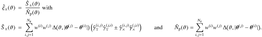 (C.22)Here,
w(i) denotes a statistical weight for the galaxy
i (which we assume to be uncorrelated with any other quantity of interest),
and Δ(ϑ,θ) denotes the bin window function (14) for a bin centred on ϑ with width
Δ(ϑ) (which we assume to be small compared to the scale on
which correlations change). Furthermore, and denote the tangential and cross component,
respectively, of the shear
estimated from the shape of galaxy i with respect to the direction
ϕ(i,j) = ϕ(θ(j) − θ(i))
defined by the positions θ(i) and
θ(j) of
galaxies i and j.
(C.22)Here,
w(i) denotes a statistical weight for the galaxy
i (which we assume to be uncorrelated with any other quantity of interest),
and Δ(ϑ,θ) denotes the bin window function (14) for a bin centred on ϑ with width
Δ(ϑ) (which we assume to be small compared to the scale on
which correlations change). Furthermore, and denote the tangential and cross component,
respectively, of the shear
estimated from the shape of galaxy i with respect to the direction
ϕ(i,j) = ϕ(θ(j) − θ(i))
defined by the positions θ(i) and
θ(j) of
galaxies i and j.
Since  for i ≠ j, the
estimator (C.22) is an unbiased estimator of
ξ ± (ϑ) (e.g., Schneider et al. 2002b):
for i ≠ j, the
estimator (C.22) is an unbiased estimator of
ξ ± (ϑ) (e.g., Schneider et al. 2002b):  (C.23)The sum
  appearing in the denominator of the shear correlation estimators (C.22) can be interpreted as the effective number of
galaxy pairs in the bin centred on ϑ. The expected effective number of pairs
Np(ϑ) in the bin reads
appearing in the denominator of the shear correlation estimators (C.22) can be interpreted as the effective number of
galaxy pairs in the bin centred on ϑ. The expected effective number of pairs
Np(ϑ) in the bin reads ![Mathematical equation: \appendix \setcounter{section}{3} \begin{eqnarray} \label{eq:mean_norm_sum} \MeanNormSum(\vartheta) &= & \EV{\NormSum(\vartheta)} = \sum_{i,j=1}^{\Ngal} \wgal^{(i)}\wgal^{(j)} \frac{1}{\AFOV^{\Ngal}}\int_{\FOV}\idiff[2]{\thetagal^{(1)}}\ldots \int_{\FOV}\idiff[2]{\thetagal^{(\Ngal)}}\, \Delta\bigl(\vartheta, \lvert \thetagal^{(j)} - \thetagal^{(i)} \rvert \bigr) \approx \frac{\ABin(\vartheta)}{\AFOV} \PairSum, \end{eqnarray}](/articles/aa/full_html/2011/12/aa17294-11/aa17294-11-eq322.png) (C.24)where
(C.24)where
![Mathematical equation: \appendix \setcounter{section}{3} \begin{equation} \ABin(\vartheta) = \frac{1}{\AFOV}\int_{\FOV}\idiff[2]{\vtheta} \int_{\FOV}\idiff[2]{\vtheta'} \Delta\bigl(\vartheta, \lvert \vtheta' - \vtheta \rvert \bigr) = 2 \pi \vartheta \varDelta(\vartheta) \end{equation}](/articles/aa/full_html/2011/12/aa17294-11/aa17294-11-eq323.png) (C.25)denote the effective bin area and
(C.25)denote the effective bin area and
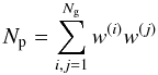 (C.26)denotes the effective total number of pairs. In the
case of uniform weights w(i) = 1
∀i, the effective number of pairs
(C.26)denotes the effective total number of pairs. In the
case of uniform weights w(i) = 1
∀i, the effective number of pairs  , and the expectation (C.24) reduces to:
 (C.27)
C.4. The covariance of the shear correlation estimators
We denote the covariance of the estimators (C.22) by:
 (C.28)To calculate c ± ± ,
we first neglect the randomness in the effective number of galaxy pairs
:
(C.28)To calculate c ± ± ,
we first neglect the randomness in the effective number of galaxy pairs
:
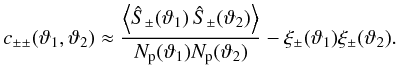 (C.29)The term
 (C.30)is then decomposed into three sums, exploiting the
symmetry of the galaxy indices and the fact that only terms with even powers of intrinsic
ellipticities contribute:
(C.30)is then decomposed into three sums, exploiting the
symmetry of the galaxy indices and the fact that only terms with even powers of intrinsic
ellipticities contribute:  (C.31)The second sum comprises terms involving two or
three distinct galaxies. The third sum contains terms involving two to four distinct galaxies.
Since all galaxies are statistically indistuingishable apart from their
weights w(i), all averages
⟨Δ(ϑ1,|θ(j) − θ(i)|)...⟩
in the same sum involving the same number of galaxies yield the same contribution to the
covariance. However, terms with different numbers of galaxies involved yield different
contributions. We neglected these differences, and thereby the noise due to the finite
sampling of the shear field in position and redshift by the galaxies (which is justified for
large Ng):
(C.31)The second sum comprises terms involving two or
three distinct galaxies. The third sum contains terms involving two to four distinct galaxies.
Since all galaxies are statistically indistuingishable apart from their
weights w(i), all averages
⟨Δ(ϑ1,|θ(j) − θ(i)|)...⟩
in the same sum involving the same number of galaxies yield the same contribution to the
covariance. However, terms with different numbers of galaxies involved yield different
contributions. We neglected these differences, and thereby the noise due to the finite
sampling of the shear field in position and redshift by the galaxies (which is justified for
large Ng): 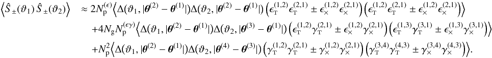 (C.32)The effective pair numbers
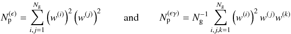 (C.33)introduced here as abbreviations become identical
to
(C.33)introduced here as abbreviations become identical
to  for uniform weights.
The covariance obtained by combining Eqs. (C.29) and (C.32) is then split into
three parts, with each part containing one of the three sums in the r.h.s. of Eq. (C.32):  (C.34)The ellipticity-noise part
 consists of all terms containing intrinsic
ellipticities, but no shear:
consists of all terms containing intrinsic
ellipticities, but no shear:  (C.35)This ellipticity-noise part obviously vanishes for
disjoint bins. The mixed part
(C.35)This ellipticity-noise part obviously vanishes for
disjoint bins. The mixed part  comprises all terms containing products of shear
and intrinsic ellipticities:
comprises all terms containing products of shear
and intrinsic ellipticities:  (C.36)The cosmic variance part
 contains all terms involving only shear:
 (C.37)We proceed by evaluating the three covariance parts
, , and for particular choices of the signs under
various assumptions about the statistics of the convergence field.
(C.37)We proceed by evaluating the three covariance parts
, , and for particular choices of the signs under
various assumptions about the statistics of the convergence field.
C.4.1. The ellipticity-noise contribution
As mentioned above,  vanishes for disjoint bins. The
ellipticity-noise contribution to the covariance of
ξ ± (ϑ) evaluates to:
vanishes for disjoint bins. The
ellipticity-noise contribution to the covariance of
ξ ± (ϑ) evaluates to:
![Mathematical equation: \appendix \setcounter{section}{3} \begin{eqnarray} c_{\pm\pm}^{(\epsilon)}(\vartheta, \vartheta) &=& \frac{2\PairSum^{(\epsilon)}}{\MeanNormSum(\vartheta)^2} \frac{\ABin(\vartheta)}{\AFOV} \Bigl\langle \left( \epsilongalt^{(1,2)} \epsilongalt^{(2,1)} \pm \epsilongalx^{(1,2)} \epsilongalx^{(2,1)} \right) \left( \epsilongalt^{(1,2)} \epsilongalt^{(2,1)} \pm \epsilongalx^{(1,2)} \epsilongalx^{(2,1)} \right) \Bigr\rangle = \frac{2\PairSum^{(\epsilon)}}{\MeanNormSum(\vartheta)^2} \frac{\ABin(\vartheta)}{\AFOV} \left[ \frac{\sigmaepsilongal^4}{4} + (\pm 1)(\pm 1) \frac{\sigmaepsilongal^4}{4} \right]\cdot \end{eqnarray}](/articles/aa/full_html/2011/12/aa17294-11/aa17294-11-eq346.png) (C.38)Hence, the ellipticity-noise part also vanishes
for non-matching signs. For uniform weights,
(C.38)Hence, the ellipticity-noise part also vanishes
for non-matching signs. For uniform weights,
 (C.39)
C.4.2. The mixed contribution
The mixed part (C.36) comprises all terms
containing products of shear and intrinsic ellipticities. After using the relations (C.19) and some trigonometry, these reduce to:
 (C.40)
 (C.41)
 (C.42)Hence,
![Mathematical equation: \appendix \setcounter{section}{3} \begin{eqnarray} c_{++}^{(\epsilon\gamma)}(\vartheta_1, \vartheta_2) &=& \frac{4 \Ngal \PairSum^{(\epsilon\gamma)}}{\MeanNormSum(\vartheta_1)\,\MeanNormSum(\vartheta_2)} \frac{1}{\AFOV^3}\int_{\FOV}\diff[2]{\thetagal^{(1)}}\int_{\FOV}\diff[2]{\thetagal^{(2)}}\int_{\FOV}\diff[2]{\thetagal^{(3)}} \Delta\bigl(\vartheta_1, \lvert \thetagal^{(2)} - \thetagal^{(1)} \rvert \bigr) \Delta\bigl(\vartheta_2, \lvert \thetagal^{(3)} - \thetagal^{(1)} \rvert \bigr) \frac{\sigmaepsilongal^2}{2} \xi_{+}\bigl(\lvert \thetagal^{(3)} - \thetagal^{(2)} \rvert \bigr) \nonumber\\&=& \frac{2\sigmaepsilongal^2\Ngal \PairSum^{(\epsilon\gamma)}}{\AFOV^2\MeanNormSum(\vartheta_1)\,\MeanNormSum(\vartheta_2)} \int_{\FOV}\diff[2]{\thetagal^{(2)}}\int_{\FOV}\diff[2]{\thetagal^{(3)}} \Delta\bigl(\vartheta_1, \lvert \thetagal^{(2)} \rvert \bigr) \Delta\bigl(\vartheta_2, \lvert \thetagal^{(3)} \rvert \bigr) \xi_{+}\bigl(\lvert \thetagal^{(3)} - \thetagal^{(2)} \rvert \bigr) \nonumber\\&=& \frac{ \Ngal^2 \PairSum^{(\epsilon\gamma)} }{ \PairSum^2} \frac{2\sigmaepsilongal^2}{\pi \ngal \AFOV} \int_{0}^{\pi}\idiff[]{\varphi_1} \xi_{+}\bigl(\lvert \vartheta_2 \uvect{0} - \vartheta_1 \uvect{\varphi_1} \rvert \bigr). \end{eqnarray}](/articles/aa/full_html/2011/12/aa17294-11/aa17294-11-eq351.png) (C.43)Here,
uϕ denotes a unit vector with
polar angle ϕ. Similar calculations yield:
(C.43)Here,
uϕ denotes a unit vector with
polar angle ϕ. Similar calculations yield:
![Mathematical equation: \appendix \setcounter{section}{3} \begin{eqnarray} c_{+-}^{(\epsilon\gamma)}(\vartheta_1, \vartheta_2) &=& \frac{ \Ngal^2 \PairSum^{(\epsilon\gamma)} }{ \PairSum^2} \frac{2\sigmaepsilongal^2}{\pi \ngal \AFOV} \int_{0}^{\pi}\idiff[]{\varphi_1} \xi_{-}\bigl(\lvert \vartheta_2 \uvect{0} - \vartheta_1 \uvect{\varphi_1} \rvert \bigr) \cos\bigl[4\varphi\bigl(\vartheta_2 \uvect{\varphi_2} - \vartheta_1 \uvect{\varphi_1}\bigr) \bigr] {\rm , and} \end{eqnarray}](/articles/aa/full_html/2011/12/aa17294-11/aa17294-11-eq352.png) (C.44)
(C.44)![Mathematical equation: \appendix \setcounter{section}{3} \begin{eqnarray} c_{--}^{(\epsilon\gamma)}(\vartheta_1, \vartheta_2) &=& \frac{ \Ngal^2 \PairSum^{(\epsilon\gamma)} }{ \PairSum^2} \frac{2\sigmaepsilongal^2}{\pi \ngal \AFOV} \int_{0}^{\pi}\idiff[]{\varphi_1} \xi_{+}\bigl(\lvert \vartheta_2 \uvect{0} - \vartheta_1 \uvect{\varphi_1} \rvert \bigr) \cos\bigl(4\varphi_1 \bigr). \end{eqnarray}](/articles/aa/full_html/2011/12/aa17294-11/aa17294-11-eq353.png) (C.45)For uniform weights, this reduces to:
(C.45)For uniform weights, this reduces to:
![Mathematical equation: \appendix \setcounter{section}{3} \begin{eqnarray} c_{++}^{(\epsilon\gamma)}(\vartheta_1, \vartheta_2) &=& \frac{2\sigmaepsilongal^2}{\pi \ngal \AFOV} \int_{0}^{\pi}\idiff[]{\varphi_1} \xi_{+}\bigl(\lvert \vartheta_2 \uvect{0} - \vartheta_1 \uvect{\varphi_1} \rvert \bigr), \end{eqnarray}](/articles/aa/full_html/2011/12/aa17294-11/aa17294-11-eq354.png) (C.46)
(C.46)![Mathematical equation: \appendix \setcounter{section}{3} \begin{eqnarray} c_{+-}^{(\epsilon\gamma)}(\vartheta_1, \vartheta_2) &=& \frac{2\sigmaepsilongal^2}{\pi \ngal \AFOV} \int_{0}^{\pi}\idiff[]{\varphi_1} \xi_{-}\bigl(\lvert \vartheta_2 \uvect{0} - \vartheta_1 \uvect{\varphi_1} \rvert \bigr) \cos\bigl[4\varphi\bigl(\vartheta_2 \uvect{\varphi_2} - \vartheta_1 \uvect{\varphi_1}\bigr) \bigr] {\rm , and} \end{eqnarray}](/articles/aa/full_html/2011/12/aa17294-11/aa17294-11-eq355.png) (C.47)
(C.47)![Mathematical equation: \appendix \setcounter{section}{3} \begin{eqnarray} c_{--}^{(\epsilon\gamma)}(\vartheta_1, \vartheta_2) &=& \frac{2\sigmaepsilongal^2}{\pi \ngal \AFOV} \int_{0}^{\pi}\idiff[]{\varphi_1} \xi_{+}\bigl(\lvert \vartheta_2 \uvect{0} - \vartheta_1 \uvect{\varphi_1} \rvert \bigr) \cos\bigl(4\varphi_1 \bigr). \end{eqnarray}](/articles/aa/full_html/2011/12/aa17294-11/aa17294-11-eq356.png) (C.48)
(C.48)
C.4.3. The cosmic variance contribution for general convergence fields
To calculate the cosmic variance contribution to the covariance, we exploit the
relations (C.15) between the empirical
correlation functions (C.12) to transform the
four-point correlations of the shear in the cosmic variance part (C.37) into four-point correlations of the
convergence: ![Mathematical equation: \appendix \setcounter{section}{3} \begin{eqnarray} \label{eq:c_pmpm_gamma_general_derivation} c_{\pm\pm}^{(\gamma)}(\vartheta_1, \vartheta_2) &=& \frac{1}{\AFOV^2\ABin(\vartheta_1)\ABin(\vartheta_2)} \int_{\FOV}\idiff[2]{\thetagal^{(1)}} \int_{\FOV}\idiff[2]{\thetagal^{(2)}} \int_{\FOV}\idiff[2]{\thetagal^{(3)}} \int_{\FOV}\idiff[2]{\thetagal^{(4)}} \Delta\bigl(\vartheta_1, \lvert \thetagal^{(2)} - \thetagal^{(1)} \rvert \bigr) \Delta\bigl(\vartheta_2, \lvert \thetagal^{(4)} - \thetagal^{(3)} \rvert \bigr) \nonumber\\&&\quad\times \Bigl\langle \Bigl[ \gammat\bigl(\thetagal^{(1)}, \thetagal^{(2)} - \thetagal^{(1)}\bigr) \gammat\bigl(\thetagal^{(2)}, \thetagal^{(2)} - \thetagal^{(1)}\bigr) \pm \gammax\bigl(\thetagal^{(1)}, \thetagal^{(2)} - \thetagal^{(1)}\bigr) \gammax\bigl(\thetagal^{(2)}, \thetagal^{(2)} - \thetagal^{(1)}\bigr) \Bigr] \nonumber\\&&\quad\times\phantom{\Bigl\langle} \Bigl[ \gammat\bigl(\thetagal^{(3)}, \thetagal^{(4)} - \thetagal^{(3)}\bigr) \gammat\bigl(\thetagal^{(4)}, \thetagal^{(4)} - \thetagal^{(3)}\bigr) \pm \gammax\bigl(\thetagal^{(3)}, \thetagal^{(4)} - \thetagal^{(3)}\bigr) \gammax\bigl(\thetagal^{(4)}, \thetagal^{(4)} - \thetagal^{(3)}\bigr) \Bigr] \Bigr\rangle_{\kappa} \, - \, \xi_{\pm}(\vartheta_1)\xi_{\pm}(\vartheta_2) \nonumber\\&=& \frac{1}{\ABin(\vartheta_1)\ABin(\vartheta_2)} \int_{\FOV}\idiff[2]{\thetagal^{(2)}} \int_{\FOV}\idiff[2]{\thetagal^{(4)}} \Delta\bigl(\vartheta_1, \lvert \thetagal^{(2)} \rvert \bigr) \Delta\bigl(\vartheta_2, \lvert \thetagal^{(4)} \rvert \bigr) \nonumber\\&&\quad\times \Biggl\langle \frac{1}{\AFOV}\int_{\FOV}\idiff[2]{\thetagal^{(1)}} \Bigl[ \gammat\bigl(\thetagal^{(1)}, \thetagal^{(2)}\bigr) \gammat\bigl(\thetagal^{(1)} + \thetagal^{(2)}, \thetagal^{(2)}\bigr) \pm \gammax\bigl(\thetagal^{(1)}, \thetagal^{(2)}\bigr) \gammax\bigl(\thetagal^{(1)} + \thetagal^{(2)}, \thetagal^{(2)}\bigr) \Bigr] \nonumber\\&&\quad\times\phantom{\Biggl\langle} \frac{1}{\AFOV}\int_{\FOV}\idiff[2]{\thetagal^{(3)}} \Bigl[ \gammat\bigl(\thetagal^{(3)}, \thetagal^{(4)}\bigr) \gammat\bigl(\thetagal^{(3)} + \thetagal^{(4)}, \thetagal^{(4)}\bigr) \pm \gammax\bigl(\thetagal^{(3)}, \thetagal^{(4)}\bigr) \gammax\bigl(\thetagal^{(3)} + \thetagal^{(4)}, \thetagal^{(4)}\bigr) \Bigr] \Biggr\rangle_{\kappa} \,-\, \xi_{\pm}(\vartheta_1)\xi_{\pm}(\vartheta_2) \nonumber\\&=& \frac{1}{\AFOV^2\ABin(\vartheta_1)\ABin(\vartheta_2)} \int_{\FOV}\idiff[2]{\thetagal^{(1)}} \int_{\FOV}\idiff[2]{\thetagal^{(2)}} \int_{\FOV}\idiff[2]{\thetagal^{(3)}} \int_{\FOV}\idiff[2]{\thetagal^{(4)}} \Delta\left(\vartheta_1, \lvert \thetagal^{(2)} \rvert \right) \Delta\left(\vartheta_2, \lvert \thetagal^{(4)} \rvert \right) \nonumber\\&&\quad\times \int_{\FOV}\idiff[2]{\thetagal^{(2)\prime}} \spavKerPM\bigl(\thetagal^{(2)}, \thetagal^{(2)\prime}\bigr) \int_{\FOV}\idiff[2]{\thetagal^{(4)\prime}} \spavKerPM\bigl(\thetagal^{(4)}, \thetagal^{(4)\prime}\bigr) \EV{ \kappa\bigl(\thetagal^{(1)}\bigr)\kappa\bigl(\thetagal^{(1)} + \thetagal^{(2)\prime} \bigr) \kappa\bigl(\thetagal^{(3)}\bigr)\kappa\bigl(\thetagal^{(3)} + \thetagal^{(4)\prime} \bigr) }_{\kappa} \,-\, \xi_{\pm}(\vartheta_1)\xi_{\pm}(\vartheta_2). \end{eqnarray}](/articles/aa/full_html/2011/12/aa17294-11/aa17294-11-eq357.png) (C.49)From the properties of the kernels
(C.49)From the properties of the kernels
 and G ± follows that
![Mathematical equation: \appendix \setcounter{section}{3} \begin{eqnarray} && \frac{1}{\ABin(\vartheta_1)} \int_{\FOV}\idiff[2]{\thetagal^{(2)}} \Delta\bigl(\vartheta_1, \lvert \thetagal^{(2)} \rvert \bigr) \int_{\FOV}\idiff[2]{\thetagal^{(2)\prime}} \spavKerPM\bigl(\thetagal^{(2)}, \thetagal^{(2)\prime}\bigr) f\bigl(\thetagal^{(2)\prime},\ldots\bigr)= \nonumber\\&&\quad \frac{1}{\ABin(\vartheta_1)} \int_{0}^{\rFOV}\idiff{\varthetagal^{(2)}} \varthetagal^{(2)} \int_{0}^{2\pi}\idiff{\varphigal^{(2)}} \int_{0}^{\rFOV}\idiff{\varthetagal^{(2)\prime}} \varthetagal^{(2)\prime} \int_{0}^{2\pi}\idiff{\varphigal^{(2)\prime}} \Delta\bigl(\vartheta_1, \varthetagal^{(2)} \bigr) \spavKerPM\bigl(\varthetagal^{(2)} \uvect{\varphigal^{(2)}}, \varthetagal^{(2)\prime} \uvect{\varphigal^{(2)\prime}}\bigr) f\bigl(\varthetagal^{(2)\prime} \uvect{\varphigal^{(2)\prime}}, \ldots\bigr) \nonumber\\&=& \frac{1}{2 \pi} \int_{0}^{2\pi}\idiff{\varphigal^{(2)}} \int_{0}^{\rFOV}\idiff{\varthetagal^{(2)\prime}} \varthetagal^{(2)\prime} \int_{0}^{2\pi}\idiff{\varphigal^{(2)\prime}} \spavKerPM\bigl(\vartheta_1 \uvect{0}, \varthetagal^{(2)\prime} \uvect{\varphigal^{(2)}}\bigr) f\bigl(\varthetagal^{(2)\prime} \uvect{\varphigal^{(2)\prime}}, \ldots\bigr) \nonumber\\&=& \frac{1}{2 \pi} \int_{0}^{\rFOV}\idiff{\varthetagal^{(2)\prime}} \varthetagal^{(2)\prime} \KerPM\bigl(\vartheta_1, \varthetagal^{(2)\prime}\bigr) \int_{0}^{2\pi}\idiff{\varphigal^{(2)\prime}} f\bigl(\varthetagal^{(2)\prime} \uvect{\varphigal^{(2)\prime}}, \ldots\bigr) \nonumber\\&=& \int_{0}^{\rFOV}\idiff{\vartheta'_1} \vartheta'_1 \KerPM \bigl(\vartheta_1, \vartheta'_1\bigr) \frac{1}{\ABin(\vartheta'_1)} \int_{\FOV}\idiff{\thetagal^{(2)\prime}} \Delta\bigl(\vartheta'_1, \lvert \thetagal^{(2)\prime} \rvert \bigr) f\bigl(\thetagal^{(2)\prime}, \ldots\bigr). \end{eqnarray}](/articles/aa/full_html/2011/12/aa17294-11/aa17294-11-eq360.png) (C.50)Thus, any contribution
can be computed from a given
(C.50)Thus, any contribution
can be computed from a given
 via a simple integral transform:
  (C.51)
C.4.4. The cosmic variance contribution for normal convergence fields
For a normal convergence field,  (C.52)and thus (exploiting the symmetries of the
integrands),
(C.52)and thus (exploiting the symmetries of the
integrands), ![Mathematical equation: \appendix \setcounter{section}{3} \begin{eqnarray} \label{eq:c_pp_gamma_normal} c_{\pm\pm}^{(\gamma)}(\vartheta_1, \vartheta_2) &&= \frac{1}{\AFOV^2\ABin(\vartheta_1)\ABin(\vartheta_2)} \int_{\FOV}\idiff[2]{\thetagal^{(1)}} \int_{\FOV}\idiff[2]{\thetagal^{(2)}} \int_{\FOV}\idiff[2]{\thetagal^{(3)}} \int_{\FOV}\idiff[2]{\thetagal^{(4)}} \Delta\left(\vartheta_1, \lvert \thetagal^{(2)} \rvert \right) \Delta\left(\vartheta_2, \lvert \thetagal^{(4)} \rvert \right) \nonumber\\ &&\quad\times \int_{\FOV}\idiff[2]{\thetagal^{(2)\prime}} \spavKerPM\bigl(\thetagal^{(2)}, \thetagal^{(2)\prime}\bigr) \int_{\FOV}\idiff[2]{\thetagal^{(4)\prime}} \spavKerPM\bigl(\thetagal^{(4)}, \thetagal^{(4)\prime}\bigr) \Bigl[ \xi_\kappa\bigl(\lvert \thetagal^{(2)\prime} \rvert\bigr) \xi_\kappa\bigl(\lvert \thetagal^{(4)\prime} \rvert\bigr) \nonumber\\ &&\quad + \xi_\kappa\bigl(\lvert \thetagal^{(3)} - \thetagal^{(1)} \rvert\bigr) \xi_\kappa\bigl(\lvert \thetagal^{(4)\prime} + \thetagal^{(3)} - \thetagal^{(2)\prime} - \thetagal^{(1)} \rvert\bigr) + \xi_\kappa\bigl(\lvert \thetagal^{(4\prime)} + \thetagal^{(3)} - \thetagal^{(1)} \rvert\bigr) \xi_\kappa\bigl(\lvert \thetagal^{(3)} - \thetagal^{(2\prime)} - \thetagal^{(1)} \rvert\bigr) \Bigr] \,-\, \xi_{\pm}(\vartheta_1)\xi_{\pm}(\vartheta_2) \nonumber\\ &&=\frac{2}{\AFOV\ABin(\vartheta_1)\ABin(\vartheta_2)} \int_{\FOV}\idiff[2]{\thetagal^{(2)}} \int_{\FOV}\idiff[2]{\thetagal^{(3)}} \int_{\FOV}\idiff[2]{\thetagal^{(4)}} \Delta\bigl(\vartheta_1, \lvert \thetagal^{(2)} \rvert \bigr) \Delta\bigl(\vartheta_2, \lvert \thetagal^{(4)} \rvert \bigr) \nonumber\\ &&\quad\times \int_{\FOV}\idiff[2]{\thetagal^{(2)\prime}} \spavKerPM\bigl(\thetagal^{(2)}, \thetagal^{(2)\prime}\bigr) \int_{\FOV}\idiff[2]{\thetagal^{(4)\prime}} \spavKerPM\bigl(\thetagal^{(4)}, \thetagal^{(4)\prime}\bigr) \xi_\kappa\bigl(\lvert \thetagal^{(3)} - \thetagal^{(2\prime)} \rvert\bigr) \xi_\kappa\bigl(\lvert \thetagal^{(3)} - \thetagal^{(4\prime)} \rvert\bigr). \end{eqnarray}](/articles/aa/full_html/2011/12/aa17294-11/aa17294-11-eq364.png) (C.53)Now, we make use of the following identity:
(C.53)Now, we make use of the following identity:
![Mathematical equation: \appendix \setcounter{section}{3} \begin{eqnarray} \label{eq:spav_xi_kappa_to_xi_m_shifted_argument} \int_{\FOV}\idiff[2]{\vtheta'}\,\spavKerM(\vtheta, \vtheta') \xi_{\kappa}(|\vtheta'' - \vtheta'|) &=& \int_{\FOV}\idiff[2]{\vtheta'}\,\spavKerM(\vtheta, \vtheta'' - \vtheta') \xi_{\kappa}(|\vtheta'|) \nonumber\\ &=& \int_{\FOV}\idiff[2]{\vtheta'}\, \frac{1}{\AFOV} \sum_{\vell} \ee^{\ii \vell \cdot (\vtheta - \vtheta'' + \vtheta')} \cos\bigl[4\varphi(\vell) - 4 \varphi(\vtheta)\bigr] \xi_{\kappa}(|\vtheta'|) \nonumber\\ &=& \cos\bigl[4\varphi(\vtheta) - 4 \varphi(\vtheta'' - \vtheta)\bigr] \int_{\FOV}\idiff[2]{\vtheta'}\, \frac{1}{\AFOV} \sum_{\vell} \ee^{\ii \vell \cdot (\vtheta'' - \vtheta - \vtheta')} \cos\bigl[4\varphi(\vell) - 4 \varphi(\vtheta'' - \vtheta)\bigr] \xi_{\kappa}(|\vtheta'|) \nonumber\\ &&\quad+ \sin\bigl[4\varphi(\vtheta) - 4 \varphi(\vtheta'' - \vtheta)\bigr] \int_{\FOV}\idiff[2]{\vtheta'}\, \frac{1}{\AFOV} \sum_{\vell} \ee^{\ii \vell \cdot (\vtheta'' - \vtheta - \vtheta')} \sin\bigl[4\varphi(\vell) - 4 \varphi(\vtheta'' - \vtheta)\bigr] \xi_{\kappa}(|\vtheta'|) \nonumber\\ &=& \cos\bigl[4\varphi(\vtheta) - 4 \varphi(\vtheta'' - \vtheta)\bigr] \xi_{-}(|\vtheta'' - \vtheta|). \end{eqnarray}](/articles/aa/full_html/2011/12/aa17294-11/aa17294-11-eq365.png) (C.54)This can be generalized to:
(C.54)This can be generalized to: ![Mathematical equation: \appendix \setcounter{section}{3} \begin{eqnarray} \label{eq:spav_xi_to_xi_shifted_argument} &&\int_{\FOV}\idiff[2]{\vtheta'}\,\spavKerPM(\vtheta, \vtheta') \xi_{\kappa}(|\vtheta'' - \vtheta'|) = \zeta_{\pm}(\vtheta, \vtheta'') {\rm , where} \end{eqnarray}](/articles/aa/full_html/2011/12/aa17294-11/aa17294-11-eq366.png) (C.55)
(C.55)![Mathematical equation: \appendix \setcounter{section}{3} \begin{eqnarray} &&\zeta_{+}(\vtheta, \vtheta'') = \xi_{+}(|\vtheta'' - \vtheta|) \quad{\rm and}\qquad \zeta_{-}(\vtheta, \vtheta'') = \xi_{-}(|\vtheta'' - \vtheta|) \cos\bigl[4\varphi(\vtheta) - 4 \varphi(\vtheta'' - \vtheta)\bigr]. \end{eqnarray}](/articles/aa/full_html/2011/12/aa17294-11/aa17294-11-eq367.png) (C.56)Hence,
(C.56)Hence,
![Mathematical equation: \appendix \setcounter{section}{3} \begin{eqnarray} c_{\pm\pm}^{(\gamma)}(\vartheta_1, \vartheta_2) &=& \frac{2}{\AFOV\ABin(\vartheta_1)\ABin(\vartheta_2)} \int_{\FOV}\idiff[2]{\thetagal^{(2)}} \int_{\FOV}\idiff[2]{\thetagal^{(3)}} \int_{\FOV}\idiff[2]{\thetagal^{(4)}} \Delta\bigl(\vartheta_1, \lvert \thetagal^{(2)} \rvert \bigr) \Delta\bigl(\vartheta_2, \lvert \thetagal^{(4)} \rvert \bigr) \zeta_{\pm}\bigl(\thetagal^{(2\prime)}, \thetagal^{(3)} \bigr) \zeta_{\pm}\bigl(\thetagal^{(4\prime)}, \thetagal^{(3)} \bigr) \nonumber\\ &=& \frac{4}{\pi\AFOV} \int_{0}^{\rFOV}\idiff{\theta_3} \theta_3 \int_{0}^{\pi}\idiff{\varphi_1} \zeta_\pm\bigl(\lvert \vartheta_1 \uvect{\varphi_1}, \theta_3 \uvect{0} \rvert\bigr) \int_{0}^{\pi}\idiff{\varphi_2} \zeta_\pm\bigl(\lvert \vartheta_2 \uvect{\varphi_2}, \theta_3 \uvect{0} \rvert\bigr). \end{eqnarray}](/articles/aa/full_html/2011/12/aa17294-11/aa17294-11-eq368.png) (C.57)
(C.57)
C.4.5. The cosmic variance contribution for zero-mean shifted log-normal convergence fields
For zero-mean shifted log-normal convergence fields, one can use Eq. (B.12) to obtain ![Mathematical equation: \appendix \setcounter{section}{3} \begin{eqnarray} \label{eq:kappa_covariance_log_normal} && \Bigl\langle \kappa\bigl(\thetagal^{(1)}\bigr) \kappa\bigl(\thetagal^{(1)} + \thetagal^{(2)} \bigr) \kappa\bigl(\thetagal^{(3)}\bigr) \kappa\bigl(\thetagal^{(3)} + \thetagal^{(4)} \bigr) \Bigr\rangle_{\kappa}= \nonumber\\[3mm] && \qquad \xi_\kappa\bigl(\lvert \thetagal^{(2)} \rvert\bigr) \xi_\kappa\bigl(\lvert \thetagal^{(4)} \rvert\bigr) + \xi_\kappa\bigl(\lvert \thetagal^{(3)} - \thetagal^{(1)} \rvert\bigr) \xi_\kappa\bigl(\lvert \thetagal^{(4)} + \thetagal^{(3)} - \thetagal^{(2)} - \thetagal^{(1)} \rvert\bigr) + \xi_\kappa\bigl(\lvert \thetagal^{(4)} + \thetagal^{(3)} - \thetagal^{(1)} \rvert\bigr) \xi_\kappa\bigl(\lvert \thetagal^{(3)} - \thetagal^{(2)} - \thetagal^{(1)} \rvert\bigr) \nonumber\\[3mm] &&\quad + \kappa_0^{-2}\left[ \xi_\kappa\bigl(\lvert \thetagal^{(2)} \rvert\bigr) \xi_\kappa\bigl(\lvert \thetagal^{(3)} - \thetagal^{(1)} \rvert\bigr) \xi_\kappa\bigl(\lvert \thetagal^{(4)} + \thetagal^{(3)} - \thetagal^{(1)} \rvert\bigr) + \ldots \right] \nonumber\\[3mm] &&\quad + \kappa_0^{-4}\left[ \xi_\kappa\bigl(\lvert \thetagal^{(2)} \rvert\bigr) \xi_\kappa\bigl(\lvert \thetagal^{(3)} - \thetagal^{(1)} \rvert\bigr) \xi_\kappa\bigl(\lvert \thetagal^{(4)} + \thetagal^{(3)} - \thetagal^{(1)} \rvert\bigr) \xi_\kappa\bigl(\lvert \thetagal^{(3)} - \thetagal^{(2)} - \thetagal^{(1)} \rvert\bigr) + \ldots \right] \nonumber\\[3mm] &&\quad + \kappa_0^{-6}\left[ \xi_\kappa\bigl(\lvert \thetagal^{(2)} \rvert\bigr) \xi_\kappa\bigl(\lvert \thetagal^{(3)} - \thetagal^{(1)} \rvert\bigr) \xi_\kappa\bigl(\lvert \thetagal^{(4)} + \thetagal^{(3)} - \thetagal^{(1)} \rvert\bigr) \xi_\kappa\bigl(\lvert \thetagal^{(3)} - \thetagal^{(2)} - \thetagal^{(1)} \rvert\bigr) \xi_\kappa\bigl(\lvert \thetagal^{(4)} + \thetagal^{(3)} - \thetagal^{(2)} - \thetagal^{(1)} \rvert\bigr) + \ldots \right] \nonumber\\[3mm] &&\quad + \kappa_0^{-8} \xi_\kappa\bigl(\lvert \thetagal^{(2)} \rvert\bigr) \xi_\kappa\bigl(\lvert \thetagal^{(3)} - \thetagal^{(1)} \rvert\bigr) \xi_\kappa\bigl(\lvert \thetagal^{(4)} + \thetagal^{(3)} - \thetagal^{(1)} \rvert\bigr) \xi_\kappa\bigl(\lvert \thetagal^{(3)} - \thetagal^{(2)} - \thetagal^{(1)} \rvert\bigr) \xi_\kappa\bigl(\lvert \thetagal^{(4)} + \thetagal^{(3)} - \thetagal^{(2)} - \thetagal^{(1)} \rvert\bigr) \xi_\kappa\bigl(\lvert \thetagal^{(4)} \rvert\bigr). \end{eqnarray}](/articles/aa/full_html/2011/12/aa17294-11/aa17294-11-eq369.png) (C.58)This reveals that the covariance for a zero-mean
shifted log-normal convergence field equals the covariance for a normal convergence field
(which consists of products of up to two correlation functions) plus “corrections” involving
products of three to six correlation functions. Inserting the correlation (C.58) into the general expression (C.51) for the cosmic
variance contribution yields (again exploiting symmetries of the integrands)
(C.58)This reveals that the covariance for a zero-mean
shifted log-normal convergence field equals the covariance for a normal convergence field
(which consists of products of up to two correlation functions) plus “corrections” involving
products of three to six correlation functions. Inserting the correlation (C.58) into the general expression (C.51) for the cosmic
variance contribution yields (again exploiting symmetries of the integrands) ![Mathematical equation: \appendix \setcounter{section}{3} \begin{eqnarray} \label{eq:c_pp_gamma_log_normal} c_{++}^{(\gamma)}(\vartheta_1, \vartheta_2) &=& \frac{1}{\AFOV^2\ABin(\vartheta_1)\ABin(\vartheta_2)} \int_{\FOV}\idiff[2]{\thetagal^{(1)}} \int_{\FOV}\idiff[2]{\thetagal^{(2)}} \int_{\FOV}\idiff[2]{\thetagal^{(3)}} \int_{\FOV}\idiff[2]{\thetagal^{(4)}} \Delta\bigl(\vartheta_1, \lvert \thetagal^{(2)} \rvert \bigr) \Delta\bigl(\vartheta_2, \lvert \thetagal^{(4)} \rvert \bigr) \nonumber\\&&\quad\times \Biggl[ \xi_\kappa\bigl(\lvert \thetagal^{(3)} - \thetagal^{(1)} \rvert\bigr) \xi_\kappa\bigl(\lvert \thetagal^{(4)} + \thetagal^{(3)} - \thetagal^{(2)} - \thetagal^{(1)} \rvert\bigr) + \xi_\kappa\bigl(\lvert \thetagal^{(4)} + \thetagal^{(3)} - \thetagal^{(1)} \rvert\bigr) \xi_\kappa\bigl(\lvert \thetagal^{(3)} - \thetagal^{(2)} - \thetagal^{(1)} \rvert\bigr) + \ldots \Biggr] \nonumber\\&=& \frac{1}{\AFOV \ABin(\vartheta_1)\ABin(\vartheta_2)} \int_{\FOV}\idiff[2]{\thetagal^{(2)}}\int_{\FOV}\idiff[2]{\thetagal^{(4)}} \int_{\FOV}\idiff[2]{\thetagal^{(3)}}\, \Delta\bigl(\vartheta_1, \lvert \thetagal^{(2)} \rvert \bigr) \Delta\bigl(\vartheta_2, \lvert \thetagal^{(4)} \rvert \bigr) \biggl\{ 4 \kappa_0^{-2} \xi_{\kappa}(\lvert \thetagal^{(2)}\rvert) \xi_{\kappa}(\lvert \thetagal^{(4)}\rvert) \xi_{\kappa}(\lvert \thetagal^{(3)}\rvert) \nonumber\\&&\quad\quad + 2 \kappa_0^{-4} \bigl[\kappa_0^2 + \xi_{\kappa}(\lvert \thetagal^{(2)}\rvert)\bigr] \xi_{\kappa}(\lvert \thetagal^{(4)}\rvert) \xi_{\kappa}(\lvert \thetagal^{(3)}\rvert) \xi_{\kappa}(\lvert \thetagal^{(3)} - \thetagal^{(2)} \rvert) \nonumber\\&&\quad\quad + 2 \kappa_0^{-4} \bigl[\kappa_0^2 + \xi_{\kappa}(\lvert \thetagal^{(4)}\rvert)\bigr] \xi_{\kappa}(\lvert \thetagal^{(2)}\rvert) \xi_{\kappa}(\lvert \thetagal^{(3)}\rvert) \xi_{\kappa}(\lvert \thetagal^{(3)} - \thetagal^{(4)} \rvert) \nonumber\\&&\quad\quad + 2 \kappa_0^{-4} \bigl[\kappa_0^2 + \xi_{\kappa}(\lvert \thetagal^{(2)}\rvert)\bigr] \bigl[\kappa_0^2 + \xi_{\kappa}(\lvert \thetagal^{(4)}\rvert)\bigr] \xi_{\kappa}(\lvert \thetagal^{(3)} - \thetagal^{(2)} \rvert) \xi_{\kappa}(\lvert \thetagal^{(3)} - \thetagal^{(4)} \rvert) \nonumber\\&&\quad\quad + 4 \kappa_0^{-6} \bigl[\kappa_0^2 + \xi_{\kappa}(\lvert \thetagal^{(2)}\rvert)\bigr] \bigl[\kappa_0^2 + \xi_{\kappa}(\lvert \thetagal^{(4)}\rvert)\bigr] \xi_{\kappa}(\lvert \thetagal^{(3)}\rvert) \xi_{\kappa}(\lvert \thetagal^{(3)} - \thetagal^{(2)} \rvert) \xi_{\kappa}(\lvert \thetagal^{(3)} - \thetagal^{(4)} \rvert) \nonumber\\&&\quad\quad + \kappa_0^{-8} \bigl[\kappa_0^2 + \xi_{\kappa}(\lvert \thetagal^{(2)}\rvert)\bigr] \bigl[\kappa_0^2 + \xi_{\kappa}(\lvert \thetagal^{(4)}\rvert)\bigr] \xi_{\kappa}(\lvert \thetagal^{(3)} \rvert) \xi_{\kappa}(\lvert \thetagal^{(3)} - \thetagal^{(2)}\rvert) \xi_{\kappa}(\lvert \thetagal^{(3)} - \thetagal^{(4)} \rvert) \xi_{\kappa}(\lvert \thetagal^{(3)} - \thetagal^{(2)} - \thetagal^{(4)} \rvert) \biggr\} \nonumber\\&&= \quad4 \kappa_0^{-2}\xi_{+}(\vartheta_1) \xi_{+}(\vartheta_2) \frac{2 \pi}{\AFOV} \int_{0}^{\rFOV}\idiff[]{\theta_3}\,\theta_3 \xi_{+}(\theta_3) \nonumber\\&&\quad + 2 \kappa_0^{-4} \bigl[\kappa_0^2 + \xi_{+}(\vartheta_1)\bigr] \xi_{+}(\vartheta_2) \frac{2}{\AFOV} \int_{0}^{\rFOV}\idiff[]{\theta_3}\, \theta_3 \xi_{+}(\theta_3) \int_{0}^{\pi}\idiff[]{\varphi_1}\, \xi_{+}(\lvert \theta_3\uvect{0} - \vartheta_1\uvect{\varphi_1} \rvert) \nonumber\\&&\quad + 2 \kappa_0^{-4} \xi_{+}(\vartheta_1) \bigl[\kappa_0^2 + \xi_{+}(\vartheta_2)\bigr] \frac{2}{\AFOV} \int_{0}^{\rFOV}\idiff[]{\theta_3}\, \theta_3 \xi_{+}(\theta_3) \int_{0}^{\pi}\idiff[]{\varphi_2}\, \xi_{+}(\lvert \theta_3\uvect{0} - \vartheta_2\uvect{\varphi_2} \rvert) \nonumber\\&&\quad + 2 \kappa_0^{-4} \bigl[\kappa_0^2 + \xi_{+}(\vartheta_1)\bigr] \bigl[\kappa_0^2 + \xi_{+}(\vartheta_2)\bigr] \frac{2}{\pi \AFOV} \int_{0}^{\rFOV}\idiff[]{\theta_3}\, \theta_3 \int_{0}^{\pi}\idiff[]{\varphi_1}\, \xi_{+}(\lvert \theta_3\uvect{0} - \vartheta_1\uvect{\varphi_1} \rvert) \int_{0}^{\pi}\idiff[]{\varphi_2}\, \xi_{+}(\lvert \theta_3\uvect{0} - \vartheta_2\uvect{\varphi_2} \rvert) \nonumber\\&&\quad + 4 \kappa_0^{-6} \bigl[\kappa_0^2 + \xi_{+}(\vartheta_1)\bigr] \bigl[\kappa_0^2 + \xi_{+}(\vartheta_2)\bigr] \frac{2}{\pi \AFOV} \int_{0}^{\rFOV}\idiff[]{\theta_3} \, \theta_3 \xi_{+}(\theta_3) \int_{0}^{\pi}\idiff[]{\varphi_1} \, \xi_{+}(\lvert \theta_3\uvect{0} - \vartheta_1\uvect{\varphi_1} \rvert) \int_{0}^{\pi}\idiff[]{\varphi_2}\, \xi_{+}(\lvert \theta_3\uvect{0} - \vartheta_2\uvect{\varphi_2} \rvert) \nonumber\\&&\quad +\kappa_0^{-8} \bigl[\kappa_0^2 + \xi_{+}(\vartheta_1)\bigr] \bigl[\kappa_0^2 + \xi_{+}(\vartheta_2)\bigr] \frac{1}{2\pi \AFOV} \int_{0}^{\rFOV}\idiff[]{\theta_3} \, \theta_3 \xi_{+}(\theta_3) \, \int_{0}^{2\pi}\idiff[]{\varphi_1} \, \xi_{+}(\lvert \theta_3\uvect{0} - \vartheta_1\uvect{\varphi_1} \rvert) \int_{0}^{2\pi}\idiff[]{\varphi_2}\, \xi_{+}(\lvert \theta_3\uvect{0} - \vartheta_2\uvect{\varphi_2} \rvert) \nonumber\\&&\quad\qquad\times \xi_{+}(\lvert \theta_3\uvect{0} - \vartheta_1\uvect{\varphi_1} - \vartheta_2\uvect{\varphi_2} \rvert). \end{eqnarray}](/articles/aa/full_html/2011/12/aa17294-11/aa17294-11-eq370.png) (C.59)The expressions for
(C.59)The expressions for
 and
and  can then be computed by combining Eqs. (C.51) and (C.59).
The expression (C.59) for a zero-mean
shifted log-normal convergence field is considerably more complicated than the corresponding
expression (C.53) for a normal convergence
field. If one only takes into account those terms in Eq. (C.59) that are also present in the case of a normal convergence field, and
the simplest term  , one obtains
![Mathematical equation: \appendix \setcounter{section}{3} \begin{equation} c^{(\gamma)}_{\pm\pm}\left(\vartheta_1, \vartheta_2 \right) = \frac{4}{\pi\AFOV} \int_{0}^{\rFOV}\idiff{\theta_3}\, \theta_3 \int_{0}^{\pi}\idiff{\varphi_1}\, \zeta_\pm\bigl(\lvert \vartheta_1 \uvect{\varphi_1}, \theta_3 \uvect{0} \rvert\bigr) \int_{0}^{\pi}\idiff{\varphi_2}\, \zeta_\pm\bigl(\lvert \vartheta_2 \uvect{\varphi_2}, \theta_3 \uvect{0} \rvert\bigr) \,+\, \xi_{\pm}(\vartheta_1) \xi_{\pm}(\vartheta_2)\frac{8 \pi}{\kappa_0^{2}\AFOV} \int_{0}^{\rFOV}\idiff[]{\theta_3}\,\theta_3\, \xi_{+}(\theta_3). \end{equation}](/articles/aa/full_html/2011/12/aa17294-11/aa17294-11-eq374.png) (C.60)
(C.60)
C.5. Shear correlation covariances for surveys comprised of several fields
So far, we have discussed the case of a survey with a single rectangular field of view. If instead the survey consists of several independent fields of the same shape and size, and with the same galaxy density, the covariances for the whole survey can be obtained by (i) computing the covariances for a single field; and (ii) dividing the result by the number of fields.
The expressions derived here for the cosmic shear covariance depend on the survey geometry
via the survey field area AF. Its inverse
 acts as an overall factor. Furthermore, the
linear dimension θF of the survey field enters as upper limit on
integrals of correlation functions. Thus, the covariances for a survey do not only depend on
the total survey area, but also on the shapes, sizes, and relative separations of the
individual fields comprising the survey (in contrast to similar expressions derived by Schneider et al. 2002a; Joachimi et al. 2008). For example, the covariances for a survey with one
4 deg2 field usually differ from the covariances for a survey with 4 independent
fields of 1 deg2.
acts as an overall factor. Furthermore, the
linear dimension θF of the survey field enters as upper limit on
integrals of correlation functions. Thus, the covariances for a survey do not only depend on
the total survey area, but also on the shapes, sizes, and relative separations of the
individual fields comprising the survey (in contrast to similar expressions derived by Schneider et al. 2002a; Joachimi et al. 2008). For example, the covariances for a survey with one
4 deg2 field usually differ from the covariances for a survey with 4 independent
fields of 1 deg2.
Appendix D: Computing shear correlations with fast Fourier transform methods
Our ray-tracing simulations provide us with the convergence and shear at positions forming a square mesh. Thus, fast Fourier transform (FFT) methods to compute their correlations are the obvious choice. Such FFT methods are so simple and efficient that they may be the best choice even for shear data sampled at irregular positions in fields with gaps and otherwise complicated geometry (as in real shear surveys), where projection of the data onto a regular mesh is required as an intermediate step.
As an illustrative example, we first revise how to use FFT methods to compute the two-point correlation of the projected galaxy density. Assume, the density contrast δg(θ) = (ng(θ) − ⟨ng⟩)/⟨ng⟩, with ng denoting the projected galaxy density and ⟨ng⟩ denoting the mean projected galaxy density, is known on a subset of points θi of a rectangular non-periodic mesh (θi), e.g. from a counts-in-cells. Some of the mesh points are allowed to have no data. To avoid aliasing, the mesh is first extended to a mesh twice as large as the original mesh in each dimension by adding mesh points around the original mesh. Let Npix denote the number of mesh points of the padded mesh.
An array
w = (w1,...,wNpix)
with a layout commensurate with the padded mesh geometry is used to store the window
function w, which holds the information on which array entries contain valid
density data and what their statistical weights (e.g. due to varying completeness) are. For
example, 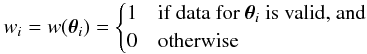 (D.1)for uniform weights. Furthermore, the weighted
density contrast data
(D.1)for uniform weights. Furthermore, the weighted
density contrast data 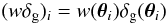 (D.2)on the mesh points
θi of the padded mesh are stored in
an array
wδg
with the same geometry as the window array w.
(D.2)on the mesh points
θi of the padded mesh are stored in
an array
wδg
with the same geometry as the window array w.
An FFT algorithm (such as, e.g., provided by FFTW, Frigo
& Johnson 2005) is used to compute the discrete Fourier transform (DFT)
 of the window array6:
  (D.3)The squared modulus of resulting array elements is
then computed,
(D.3)The squared modulus of resulting array elements is
then computed,  (D.4)and transformed back to configuration space to
obtain the spatial auto-correlation
(D.4)and transformed back to configuration space to
obtain the spatial auto-correlation  of the window function array:
  (D.5)Here,
 (D.6)The auto-correlation
 of the weighted density contrast is computed in the same way with FFTs. Finally, the
correlations are binned into radial bins to obtain the text-book counts-in-cells
Landy-&-Szalay estimator for the angular two-point
correlation ξgal of galaxies:
of the weighted density contrast is computed in the same way with FFTs. Finally, the
correlations are binned into radial bins to obtain the text-book counts-in-cells
Landy-&-Szalay estimator for the angular two-point
correlation ξgal of galaxies:
 (D.7)where Δ(ϑ,θ) denotes the bin
function (14).
(D.7)where Δ(ϑ,θ) denotes the bin
function (14).
With the same approach, one can calculate estimates for convergence and shear correlations.
One creates arrays w, wκ,
wγ1,
and
wγ2
storing the values of the window function and the weighted convergence and shear components on
the points θi of the padded mesh. One
then uses FFTs to compute the auto-correlation  of the window function, the auto-correlation
  of the weighted convergence, and the auto- and cross-correlations
 of the weighted shear components. Finally, the correlations are binned into radial bins to
estimate the isotropic correlations:
of the weighted shear components. Finally, the correlations are binned into radial bins to
estimate the isotropic correlations:  (D.8)
(D.8)![Mathematical equation: \appendix \setcounter{section}{4} \begin{eqnarray} \est{\xi}_+(\vartheta) &=& \frac{\sum_i \Delta\bigl(\vartheta, \lvert \vtheta_i\rvert \bigr) \left[\bar{S}_{\vect{w\gamma_1}, \vect{w\gamma_1}, i} + \bar{S}_{\vect{w\gamma_2}, \vect{w\gamma_2}, i} \right]} {\sum_i \Delta\bigl(\vartheta, \lvert \vtheta_i\rvert \bigr) \bar{S}_{\vect{w}, \vect{w}, i}} \nonumber\\&=& \frac{\sum_{ij} \Delta\bigl(\vartheta, \lvert \vtheta_j - \vtheta_i \rvert \bigr) w(\vtheta_i) w(\vtheta_j) \left[ \gammat(\vtheta_i, \vtheta_j - \vtheta_i) \gammat(\vtheta_j, \vtheta_j - \vtheta_i) + \gammax(\vtheta_i, \vtheta_j - \vtheta_i) \gammax(\vtheta_j, \vtheta_j - \vtheta_i) \right]} {\sum_{ij} \Delta\bigl(\vartheta, \lvert \vtheta_j - \vtheta_i \rvert \bigr) w(\vtheta_i) w(\vtheta_j)}, \end{eqnarray}](/articles/aa/full_html/2011/12/aa17294-11/aa17294-11-eq406.png) (D.9)
(D.9)![Mathematical equation: \appendix \setcounter{section}{4} \begin{eqnarray} \est{\xi}_-(\vartheta) &=& \frac{\sum_i \Delta\bigl(\vartheta, \lvert \vtheta_i\rvert \bigr) \left\{ \cos\bigl[4 \varphi(\vtheta_i)\bigr] \bar{S}_{\vect{w\gamma_1}, \vect{w\gamma_1}, i} - \cos\bigl[4 \varphi(\vtheta_i)\bigr] \bar{S}_{\vect{w\gamma_2}, \vect{w\gamma_2}, i} +2\sin\bigl[4 \varphi(\vtheta_i)\bigr] \bar{S}_{\vect{w\gamma_1}, \vect{w\gamma_2}, i} \right\}} {\sum_i \Delta\bigl(\vartheta, \lvert \vtheta_i\rvert \bigr) \bar{S}_{\vect{w}, \vect{w}}(\vtheta_i)} \nonumber\\&=& \frac{\sum_{ij} \Delta\bigl(\vartheta, \lvert \vtheta_j - \vtheta_i \rvert \bigr) w(\vtheta_i) w(\vtheta_j) \left[ \gammat(\vtheta_i, \vtheta_j - \vtheta_i) \gammat(\vtheta_j, \vtheta_j - \vtheta_i) - \gammax(\vtheta_i, \vtheta_j - \vtheta_i) \gammax(\vtheta_j, \vtheta_j - \vtheta_i) \right]} {\sum_{ij} \Delta\bigl(\vartheta, \lvert \vtheta_j - \vtheta_i \rvert \bigr) w(\vtheta_i) w(\vtheta_j)}\cdot \end{eqnarray}](/articles/aa/full_html/2011/12/aa17294-11/aa17294-11-eq407.png) (D.10)FFT methods can also be used to compute
galaxy-galaxy lensing statistics. For example, an estimator for the average tangential shear
profile ⟨γt⟩(ϑ) around a sample of lens
galaxies as measured in a sample of source galaxies reads:
(D.10)FFT methods can also be used to compute
galaxy-galaxy lensing statistics. For example, an estimator for the average tangential shear
profile ⟨γt⟩(ϑ) around a sample of lens
galaxies as measured in a sample of source galaxies reads:
![Mathematical equation: \appendix \setcounter{section}{4} \begin{equation} \bEV{\est{\gammat}}(\vartheta) = - \frac{\sum_i \Delta\bigl(\vartheta, \lvert \vtheta_i\rvert \bigr)\left\{ \cos\bigl[2 \varphi(\vtheta_i)\bigr] \bar{S}_{\vect{w_{{\rm l}} n_{{\rm l}}}, \vect{w_{{\rm s}} n_{{\rm s}} \gamma_1}, i} + \sin\bigl[2 \varphi(\vtheta_i)\bigr] \bar{S}_{\vect{w_{{\rm l}} n_{{\rm l}}}, \vect{w_{{\rm s}} n_{{\rm s}} \gamma_2}, i} \right\}} {\sum_i \Delta\bigl(\vartheta, \lvert \vtheta_i\rvert \bigr) \bar{S}_{\vect{w_{{\rm l}} n_{{\rm l}}}, \vect{w_{{\rm s}} n_{{\rm s}}}, i}}, \end{equation}](/articles/aa/full_html/2011/12/aa17294-11/aa17294-11-eq409.png) (D.11)where wl,
nl, ws, and
ns denote the weights and densities of the lens and source galaxy
samples.
(D.11)where wl,
nl, ws, and
ns denote the weights and densities of the lens and source galaxy
samples.
All Tables
All Figures
|
Fig. 1 The pdf pκ(κ) of the convergence κ for sources with median redshift zmedian = 1. The pdf measured from the simulations (solid line) is compared to a zero-mean normal distribution with matching variance (dashed line), and the best-fitting zero-mean shifted log-normal distribution (dotted line). |
| In the text | |
|
Fig. 2 The minimum-convergence parameter κ0 as a function of source redshift z (obtained from fits to the pdf of the convergence for sources at redshift z). |
| In the text | |
|
Fig. 3 The convergence correlation ξκ(ϑ) (squares) and the cosmic shear correlations ξ + (ϑ) (diamonds) and ξ−(ϑ) (triangles) as functions of the angular scale ϑ for sources with median redshift zmedian = 1 measured from the simulations. Error bars indicate uncertainties on the mean estimated from the field-to-field variance of the simulated fields. Also shown are the analytic fits (see text) to the correlations ξ + (ϑ) (dashed line) and ξ−(ϑ) (dotted line). |
| In the text | |
|
Fig. 4 The cosmic variance contributions |
| In the text | |
|
Fig. 5 The cosmic variance contributions |
| In the text | |
|
Fig. 6 Joint posterior distributions of the mean matter density Ωm and the matter power spectrum normalization σ8 of a flat ΛCDM universe inferred from a cosmic shear survey with ng = 25 arcmin-2 (assuming flat priors for Ωm and σ8, and all other cosmological parameters known). Shown are the 68% (inner) and 95% (outer) confidence contours for a small survey in 5 fields of 2 × 2 deg2 (left panels), a survey in 6 fields of 4 × 4 deg2 (middle panels), and a large survey in a 120 × 120 deg2 field (right panels) obtained when using the covariance matrix measured from our lensing simulations (solid lines), the normal approximation (top, dashed lines), the log-normal approximation (top, dotted lines), the empirical corrections to the normal approximation by Semboloni et al. (2007, bottom, and the corrections by Sato et al. (2011b, bottom. |
| In the text | |
|
Fig. 7 68% (inner) and 95% (outer) confidence contours of the joint posterior distributions of the mean matter density Ωm and the matter power spectrum normalization σ8 of a flat ΛCDM universe inferred from a cosmic shear survey with ng = 70 arcmin-2 in 5 fields of 2 × 2 deg2, obtained using the covariance from our lensing simulations (solid lines), the normal approximation (top, dashed lines), the log-normal approximation (top, dotted lines), the empirical corrections to the normal approximation by Semboloni et al. (2007, bottom, and the corrections by Sato et al. (2011b, bottom. For the left panels, the cosmic covariance parts of the data covariance matrices have be used as given by the approximations. For the right panels, the cosmic variance parts have been modified where needed to ensure positive-semidefiniteness (see text for details). |
| In the text | |
Current usage metrics show cumulative count of Article Views (full-text article views including HTML views, PDF and ePub downloads, according to the available data) and Abstracts Views on Vision4Press platform.
Data correspond to usage on the plateform after 2015. The current usage metrics is available 48-96 hours after online publication and is updated daily on week days.
Initial download of the metrics may take a while.