| Issue |
A&A
Volume 535, November 2011
|
|
|---|---|---|
| Article Number | A107 | |
| Number of page(s) | 18 | |
| Section | Galactic structure, stellar clusters and populations | |
| DOI | https://doi.org/10.1051/0004-6361/201117373 | |
| Published online | 21 November 2011 | |
A spectroscopic survey of thick disc stars outside the solar neighbourhood⋆,⋆⋆
1
Université de Nice Sophia Antipolis, CNRS, Observatoire de la Côte d’Azur,
Cassiopée UMR 6202,
BP 4229,
06304
Nice,
France
e-mail: georges.kordopatis@oca.eu
2
Institute of Astronomy, University of Cambridge,
Madingley Road,
Cambridge
CB3 0HA,
UK
3
Johns Hopkins University, Baltimore, MD, USA
4
Kapteyn Astronomical Institute, University of Groningen,
PO Box 800,
9700 AV
Groningen, The
Netherlands
5
Departamento de Astronomía y Astrofísica, Pontificia Universidad
Católica de Chile, Av. Vicuña
Mackenna 4860, Casilla 306, Santiago 22, Chile
6
Université de Strasbourg, Observatoire Astronomique,
Strasbourg,
France
Received:
30
May
2011
Accepted:
3
October
2011
Context. In the era of large spectroscopic surveys, Galactic archaeology aims to understand the formation and evolution of the Milky Way by means of large datasets. In particular, the kinematic and chemical study of the thick disc can give valuable information on the merging history of the Milky Way.
Aims. Our aim is to detect and characterise the Galactic thick disc chemically and dynamically by analysing F, G, and K stars, whose atmospheres reflect their initial chemical composition.
Methods. We performed a spectroscopic survey of nearly 700 stars probing the Galactic thick disc far from the solar neighbourhood towards the Galactic coordinates (l ~ 277°, b ~ 47°). The derived effective temperatures, surface gravities and overall metallicities were then combined with stellar evolution isochrones, radial velocities and proper motions to derive the distances, kinematics and orbital parameters of the sample stars. The targets belonging to each Galactic component (thin disc, thick disc, halo) were selected either on their kinematics or according to their position above the Galactic plane, and the vertical gradients were also estimated.
Results. We present here atmospheric parameters, distances and kinematics for this sample and a comparison of our kinematic and metallicity distributions with the Besançon model of the Milky Way. The thick disc far from the solar neighbourhood is found to differ only slightly from the thick disc properties as derived in the solar vicinity. For regions where the thick disc dominates (1 ≲ Z ≲ 4 kpc), we measured vertical velocity and metallicity trends of ∂Vφ/∂Z = 19 ± 8 km s-1 kpc-1 and ∂ [M/H] /∂Z = −0.14 ± 0.05 dex kpc-1, respectively. These trends can be explained as a smooth transition between the different Galactic components, although intrinsic gradients could not be excluded. In addition, a correlation ∂Vφ/∂ [M/H] = −45 ± 12 km s-1 dex-1 between the orbital velocity and the metallicity of the thick disc is detected. This gradient is inconsistent with the SDSS photometric survey analysis, which did not detect any such trend, and challenges radial migration models of thick disc formation. Estimations of the scale heights and scale lengths for different metallicity bins of the thick disc result in consistent values, with hR ~ 3.4 ± 0.7 kpc, and hZ ~ 694 ± 45 pc, showing no evidence of relics of destroyed massive satellites.
Key words: Galaxy: evolution / Galaxy: kinematics and dynamics / stars: abundances / methods: observational
Based on VLT/FLAMES observations collected at the European Southern Observatory, proposals 075.B-0610-A & 077.B-0.382.
Full Tables 1, 2, and 4 are only available at the CDS via anonymous ftp to cdsarc.u-strasbg.fr (130.79.128.5) or via http://cdsarc.u-strasbg.fr/viz-bin/qcat?J/A+A/535/A107
© ESO, 2011
1. Introduction
In the paradigm of a dark energy and dark matter dominated Universe, the process of disc galaxy formation is still very poorly understood. For instance, the creation of the Galactic thick disc still remains a riddle. Was it formed by the accretion of satellites that have deposited their debris in a roughly planar configuration (Abadi et al. 2003), or was the thin disc heated after successive small accretions as suggested for example by Villalobos & Helmi (2008)? Did the thick disc stars form in situ, through heating of the thin disc by gas rich mergers and starburst during the merger process (Brook et al. 2004), or did they migrate because of resonances with the spiral arms (and the central bar), as suggested for example by Schönrich & Binney (2009) or Loebman et al. (2011)?
To answer these questions, we would ideally like to tag or associate the visible components of the Galaxy to parts of the proto-Galactic hierarchy. All necessary constraints can be obtained from a detailed analysis of the chemical abundances of cool and intermediate temperature stars. Indeed, F, G, and K type dwarf stars are particularly useful to study Galactic evolution, because they are both numerous and long-lived, and their atmospheres reflect their initial chemical composition. However, a direct measurement of their spatial distribution requires accurate estimates of stellar distances, which is a delicate step involving (if the parallax is not available) the determination of precise stellar parameters (effective temperatures, surface gravities and metal content).
That is the reason why most spectroscopic surveys of the thick disc up to now are restricted to the solar neighbourhood (within about a 500 pc radius), except for those with relatively few stars in their samples. Nevertheless, detailed metallicity measurements based on such spectroscopic observations of kinematically selected thick disc stars revealed in several studies a clear distinction in chemical elements ratios between the metal-poor tails of the thin and the thick discs (Edvardsson et al. 1993; Bensby & Feltzing 2006; Reddy et al. 2006; Fuhrmann 2008; Ruchti et al. 2010; Navarro et al. 2011). Stars belonging to the latter are α-enhanced, suggesting a rapid formation of the thick disc and a distinct chemical history. Indeed, the [α/Fe] chemical index is commonly used to trace the star formation time-scale in a system in terms of the distinct roles played by supernovae (SNe) of different types in the Galactic enrichment. The α-elements are produced mainly during Type II SNe explosions of massive stars (M > 8 M⊙) on a short time-scale (~107 years), whereas iron is also produced by Type Ia SNe of less massive stars on a much longer time-scale (~109 years).
On the other hand, photometric surveys such as the SDSS (York et al. 2000) explore a much larger volume, but suffer from greater uncertainties in the derived parameters. Based on photometric metallicities and distances of more than 2 million F/G stars up to 8 kpc from the Sun, Ivezić et al. (2008) suggested that the transition between the thin and the thick disc can be modelled as smooth, vertical shifts of metallicity and velocity distributions, challenging the view of two distinct populations that was introduced by Gilmore & Reid (1983).
The goal of this paper is to put additional constraints on the vertical properties of the thick disc. For that purpose, we spectroscopically explored the stellar contents outside the solar neighbourhood using the Ojha et al. (1996) catalogue. The authors of that survey photometrically observed several thousands of stars towards the direction of Galactic antirotation. They provide the Johnson U, B, V magnitudes as well as the proper motions for most of the targets up to V ~ 18.5 mag. We selected 689 of them based on their magnitudes to probe the Galactic thick disc, and observed them using the VLT/FLAMES GIRAFFE spectrograph in the LR08 setup (covering the infrared ionized calcium triplet).
The line-of-sight (l ~ 277°, b ~ 47°) was chosen in accordance to results found by Gilmore et al. (2002) towards (l ~ 270°, b ~ −45°) and (l ~ 270°, b ~ 33°) that were confirmed by Wyse et al. (2006) towards (l ~ 260°, b ~ −23°), (l ~ 104°, b ~ 45°), (l ~ 86°, b ~ 35°), which state that thick disc stars farther than 2 kpc from the Sun seem to have a rotational lag greater than the canonical thick disc. Indeed, it is commonly accepted that the latter lags the local standard of rest (LSR) by ~50 km s-1, whereas the authors cited above found a lag twice as high (~100 km s-1) at long distances. Because the angular momentum is essentially a conserved quantity in galaxy formation, this lagging sub-population has been suggested by the authors to be the remnants of the last major merger of the Milky Way, back to z ~ 2.
For the analysis of this very substantial sample of FLAMES spectra we used the pipeline presented in Kordopatis et al. (2011, hereafter Paper I). It allowed us to obtain the effective temperature (Teff), the surface gravity (log g) and the overall metallicity1 ([M/H]) for the stars of our sample. They were combined with the proper motions and the (B − V) colours of the Ojha catalogue and our derived radial velocities. Those parameters were then used to estimate the distances, galactocentric positions and kinematics, as well as the orbital parameters (eccentricities, apocentric and pericentric distances, angular momenta) of our targets.
The structure of this paper is as follows. The observed stellar sample is presented in the next section together with the data reduction and the radial velocity derivation. The method used to determine the atmospheric parameters is reviewed in Sect. 3. In Sect. 4 the estimates for the atmospheric parameters, the distances and the kinematics are presented. In Sect. 5 a clean sample of stars is selected, whose stars are analysed in Sect. 6 with respect to their distance above the Galactic plane; then we compare them to the Besançon model of the Milky Way (Robin et al. 2003). The Galactic components, chosen with a probabilistic approach and according to their distance above the Galactic plane, are also characterised and discussed in relation with thick disc formation scenarios. Finally, we estimate in Sect. 7 the radial scale lengths and scale heights of the thin disc and the thick disc.
2. Observations, data reduction and radial velocity derivation
The observations were obtained with VLT/FLAMES feeding the GIRAFFE spectrograph in MEDUSA mode, that allows a simultaneous allocation of 132 fibres (including sky). The GIRAFFE low-resolution grating LR08 (8206–9400 Å, R ~ 6500, sampling = 0.2 Å) was used during ESO observing periods 75 and 77 (2005 and 2006, respectively). One of the interesting points of that configuration is that it contains the Gaia/RVS wavelength range (8475–8745 Å), and is similar to its low-resolution mode (R ~ 7000).
In that wavelength range the IR Ca ii triplet (8498.02, 8542.09, 8662.14 Å) is predominant for most spectral types and luminosity classes even for very metal-poor stars (see, for example Zwitter et al. 2004). In addition, these strong features are still detectable even at low signal-to-noise ratio (S/N), allowing a good radial velocity (Vrad) derivation and an overall metallicity estimation. Paschen lines (for example 8502.5, 8545.4, 8598.4, 8665.0 Å) are visible for stars hotter than G3. The Mg i (8807 Å) line, which is a useful indicator of surface gravity (see Ruck & Smith 1993), is also visible even for low S/N. Finally, molecular lines such as TiO and CN can be seen for cooler stars.
The 689 stars of our sample were selected only from their V-magnitudes and the availability of proper motions measurements in the catalogue of Ojha et al. (1996). They were faint enough to probe the Galactic thick disc and bright enough to have acceptable S/N (mV ≤ 18.5 mag). To fill all available fibres of MEDUSA, brighter stars in the Ojha catalogue were added to our survey (mV ≥ 14), resulting in a bimodal distribution in magnitudes. We made no colour selection, which resulted in a wide range of both log g and Teff as we will show in Sects. 3 and 4. The magnitude precisions range from 0.02 mag for the brightest, to 0.05 mag for the faintest stars (Ojha et al. 1996). Associated errors for the proper motions are estimated to be 2 mas year-1.
Eight different fields were observed with two exposures each. The spectra were reduced using the Gasgano ESO GIRAFFE pipeline2 (version 2.3.0, Izzo et al. 2004) with optimal extraction. The sky-lines were removed from our spectra using the software developed by M. Irwin (Battaglia et al. 2006), which is optimal for the wavelength range around the IR Ca ii triplet. For each field the four fibres that were allocated to the sky were combined to obtain a median sky spectrum and separate the continuum from the sky-line components. Then, the latter was cross-correlated to the object spectrum (which was also split into continuum and line components) to match the object sky-line intensities and positions. Afterwards, the sky was subtracted by finding the optimal scale factor between the masked sky-line and the object spectrum. Individual exposures were then cross-correlated using IRAF to put them on the same reference frame and to be summed. Before summing them, the cosmic rays and the remaining residual sky-lines were removed by comparing the flux levels of the individual exposures.
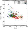 |
Fig. 1 Radial velocity uncertainties versus the (B − V) colour for the final catalogue (479 stars), as selected in Sect. 5. Dots with different colours refer to different metallicity ranges. |
To measure the radial velocities we used a binary mask of a K0 type star at the LR08 resolution (available from the Geneva observatory with the girBLDRS routine, see Royer et al. 2002). The cross-correlation function (CCF) between the observed spectra and the binary mask was computed, extracting from the position of the peak the Vrad value. The spectral features corresponding to the full-width at half-maximum (FWHM) of the Ca ii triplet and the Mg i (8807 Å) lines were added manually into this binary mask, because we found that otherwise the cross-correlation routine did not converge for the lowest S/N spectra (where the spectral lines are hard to identify). The wider lines added to the binary mask play a dominant role in the cross-correlation method. This implies that no particular concern has to be raised about errors caused by possible template mismatches. The only expected effect is a decrease in the precision of the Vrad estimates, owing to a broader CCF. Nevertheless, as shown in Paper I, the derivation of the atmospheric parameters is not altered as long as the uncertainties in Vrad are less then ~7–8 km s-1. We found in our survey that the mean error on the Vrad is 4.70 km s-1 and the standard deviation of the error distribution is 1.3 km s-1. In Fig. 1 we plot the estimated errors on the radial velocities versus the (B − V) colour of the targets. A colour code was added according to the derived metallicity of the stars (as found in Sect. 3). The largest errors are found for the hotter and the most metal-poor stars, as expected, because the mixture of broader lines for the former and weaker lines for the latter differ the most. The individual values of the heliocentric Vrad are presented in Table 1 and will be used in Sect. 4.3 to determine the galactocentric velocities and hence the orbits of the stars.
Kinematics of the selected targets belonging to the final catalogue.
Individual atmospheric parameters (as derived by the procedure of Paper I), relative V-Magnitudes, (B − V) colour, absolute V-magnitude and estimated S/N of the observed targets of the final catalogue.
The spectra were then shifted at the rest frame and linearly rebinned by a factor of two, in agreement with Shannon’s criterion. Furthermore, they were resampled to match the sampling of the synthetic spectra library we had in our possession, which we used to derive the atmospheric parameters (see Paper I). This led to a final sampling of 0.4 Å and an increased S/N per pixel.
Then the spectra were cut at the wavelengths 8400–8820 Å to keep the range with the predominant lines and suffering least by CCD spurious effects (border effects, presence of a glow in the red part) and possible sky residuals. For this reason, the range between 8775 and 8801 Å which contains few iron lines compared to the possible important sky residuals, was also removed. The spectral feature corresponding to the Mg i around ~8807 Å was nevertheless kept. The cores of the strong Ca ii lines were also removed, as explained in Paper I.
The final spectra, containing 957 pixels, were normalised by iteratively fitting a second-order polynomial to the pseudo-continuum, asymmetrically clipping off points that lay far from the fitting curve. This first normalisation is not very crucial, because the pipeline that derives the atmospheric parameters renormalises the spectra with the aid of synthetic spectra (see Paper I).
Finally, the binary stars or suspected ones, and very low quality spectra (owing to a bad location of the fibre on the target) were removed at this point from the rest of the sample, leading to a final sample of 636 stars. The final measured S/N of our spectra varies from ~5 to ~200 pixel-1, with a mean of ~70 pixel-1. Nevertheless, the cumulative smoothing effects of spectral interpolation and resampling lead to an over-estimation of the S/N by a factor of ~1.4 because of the pixel correlation. Hence, the plot of Fig. 2 shows the apparent magnitude versus the corrected S/N.
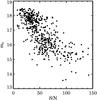 |
Fig. 2 Apparent magnitude mv versus measured signal-to-noise ratio (per pixel) for all observed sample (689 stars in total). |
3. Determination of the stellar atmospheric parameters
We used the procedure described in Paper I to derive the atmospheric parameters of the stars and their associated errors. To take into account the overestimation of the S/N owing to the pixel resampling, the measured S/N was decreased by a factor 1.4 at each step of the pipeline. The obtained parameter values are shown in Table 2.
We recall that this procedure consists of using two different algorithms simultaneously, MATISSE (Recio-Blanco et al. 2006) and DEGAS (Bijaoui et al. 2010), to iteratively renormalise the spectra and derive the atmospheric parameters of the observed targets. The learning phase for the algorithms is based on a grid of synthetic spectra covering Teff from 3000 K to 8000 K, log g from 0 to 5 (cm s-2) and [M/H] from −5 dex to +1.0 dex. A coupling between the overall metallicity and the α element abundances3 is assumed according to the commonly observed enhancements in metal-poor Galactic stars:
-
[α/Fe] = 0.0 dex for [M/H] ≥ 0.0 dex;
-
[α/Fe] = −0.4 × [M/H] dex for −1 ≤ [M/H] < 0 dex;
-
[α/Fe] = +0.4 dex for [M/H] ≤ −1.0 dex.
At S/N ~ 50 pixel-1 the pipeline returns typical errors4 for stars with log g ≥ 3.9 and −0.5 < [M/H] ≤ −0.25 dex, of 70 K, 0.12 dex, 0.09 dex for Teff, log g and [M/H], respectively. For more metal-poor stars (−1.5 < [M/H] ≤ −0.5 dex) the achieved accuracies are 108 K, 0.17 dex and 0.12 dex. Finally, for stars classified as halo giants (Teff < 6000 K, log g < 3.5, −2.5 < [M/H] ≤ −1.25 dex) the typical errors are 94 K, 0.28 dex and 0.17 dex (see Paper I).
This pipeline was successfully tested on the observed stellar libraries of S4N (Allende Prieto et al. 2004) and CFLIB (Valdes et al. 2004), showing no particular biases in Teff or log g. Still, a bias of −0.1 dex was found for metal-rich dwarfs, which, as discussed in Paper I, we decided not to correct because of the small range of log g and [M/H] spanned by the libraries. As discussed in Sect. 4.1, this possible bias is not expected to introduce any significant bias in the distance estimates or the derived velocities of the present survey.
4. Determination of the stellar distances, kinematics and orbits
Typical F, G and K main-sequence stars have mv ~ 15−18 at distances of 1–5 kpc, and at least until the ESA/Gaia mission, stellar distances for targets far from the solar neighbourhood have to be determined spectroscopically or photometrically. For instance, the atmospheric parameters determined in the previous section can be projected onto a set of theoretical isochrones to derive the absolute magnitudes of the stars. Then we can derive the line-of-sight distances using the distance modulus.
4.1. Procedure to estimate stellar distances
We generated our own set of isochrones by using the YYmix2 interpolation code, based on the Yonsei-Yale (Y2) models (version 2, Demarque et al. 2004) combined with the Lejeune et al. (1998) colour table.
We set the youngest age of the isochrones at 2 Gyr, because we expect to observe targets from the old thin disc, the thick disc and the halo, and very few stars are expected to be younger than this. Following Zwitter et al. (2010), we generated isochrones with a constant step of 1 Gyr, up to 14 Gyr. In addition, we used the full metallicity range of the Y2 models, ranging from [Fe/H]= −3.0 dex to [Fe/H] = +0.8 dex. The step in metallicity is constant, equal to 0.1 dex, smaller than the typical error on the derived metallicities of the observed stars. The adopted values for the α-enhancements at different metallicities are the same as those used for the grid of synthetic spectra described in the previous section. At the end, a set of 494 isochrones were generated.
To obtain the absolute magnitude Mv, we used the method of
Zwitter et al. (2010). This procedure consists of
finding the most likely values of the stellar parameters, given the measured atmospheric
ones, and the time spent by a star in each region of the H–R diagram. In practice, we
selected the subset of isochrones with [M/H] ± Δ [M/H] , where
Δ [M/H] is the estimated error on the metallicity, for each set of
derived Teff, log g and [M/H]. Then a
Gaussian weight was associated to each point of the selected isochrones, which depends on
the measured atmospheric parameters and the considered errors (see Eq. (1)). This criterion allows the algorithm to
select only the points whose values are close to those derived by the pipeline. Still, in
low S/N spectra, whose parameter errors can be
significant, an excessive weight can be appointed to rapid evolutionary phases of the
isochrones, where it is unlikely that there are many stars. To avoid this artefact, we
associate to the previous weight, another one, that is proportional to the time spent by a
star on each part of the H–R diagram. Following Zwitter
et al. (2010), this weight was set as dm: the mass step between
two points of the same isochrone. Hence, the total weight W for each
point on the isochrone can be expressed as follows:  (1)where i
corresponds to Teff, log g, [M/H] or
(B − V),
θi to the parameter values of the points on
the isochrones,
(1)where i
corresponds to Teff, log g, [M/H] or
(B − V),
θi to the parameter values of the points on
the isochrones,  to the values derived from observations (from photometry or spectroscopy) and
 to the associated error of the measurement. The absolute magnitude
Mv is then obtained by computing the weighted mean of all
points of the subset of isochrones. The corresponding error is computed by considering the
standard deviation of the latter.
to the associated error of the measurement. The absolute magnitude
Mv is then obtained by computing the weighted mean of all
points of the subset of isochrones. The corresponding error is computed by considering the
standard deviation of the latter.
To test the adopted procedure, we made extensive use of the Besançon model of the Milky Way (Robin et al. 2003). This is a semi-empirical model that includes physical constraints and current knowledge of the formation and evolution of the Galaxy to return for a given line-of-sight (los) the atmospheric parameters, the positions and the kinematics of simulated stars in a given range of magnitudes. It uses the isochrones of Schaller et al. (1992) to simulate the stellar populations of the thin disc and the isochrones of Bergbusch & Vandenberg (1992) to simulate the thick disc and the halo. Thus, small offsets may be expected when comparing the distances we derived with the Y2 isochrones and those deduced from this model.
We obtained a simulated catalogue of ~4 × 10³ stars towards (l ~ 277°, b ~ 47°) in this way and tested the method by computing the los distances of the targets in two ways:
-
1.
The Besançon atmospheric parameter values were taken and associated with errors that the pipeline of Paper I would produce for the corresponding stellar type and metallicity at different S/N. In that way we checked the impact of the weight W of Eq. (1) on the distance estimation. We represented in the first row of Table 3 the values at 70% of the error distribution that we found. The results are very encouraging because at S/N ~ 20 pixel-1 the dispersion of the recovered distances with respect to the theoretical ones is only 27%. Nevertheless, a bias was found for stars farther than ~8 kpc, even at high S/N. For instance, at S/N ~ 50 pixel-1 the distances for the farthest stars are overestimated by ~18%, and this offset increases with decreasing S/N (up to 30% at S/N ~ 10 pixel-1). Indeed, these distant stars are found to be metal-poor giants (halo stars), for which the errors in the atmospheric parameters are expected to be larger (e.g.: at S/N ~ 20 pixel-1, the uncertainties are 188 K, 0.57 dex and 0.23 dex for Teff, log g and [M/H], respectively). These uncertainties will allow a high number of points on the isochrones to have roughly the same weight W and to span a relatively wide range of magnitudes, because the late-type giant stars have a sensitive dependance of absolute magnitude with astrophysical parameters. This effect will result in a mean Mv that will be lower, designating the stars to a farther distance than they should be. This problem is well known and has already been described in detail in Breddels et al. (2010) and Zwitter et al. (2010). As we will see in Sect. 6.2.3, it will concern less than 4% of our observed sample. A disagreement of ~13% towards smaller distances for the stars closer than 1 kpc was found. This difference is caused by the different sets of isochrones involved, and not by the method itself. Indeed, we verified that the absolute magnitudes for main-sequence stars at a given metallicity were always higher in the case of Schaller et al. (1992) compared to the Y2 ones. The difference disappeared for the dwarfs generated from the isochrones of Bergbusch & Vandenberg (1992).
-
2.
The parameters derived from the spectra of the pseudo-stars were taken. For that purpose, we computed degraded (S/N ~ 100, 50, 20, 10 pixel-1) synthetic spectra with the atmospheric parameters of the simulated targets and used the automated pipeline to derive their Teff, log g and [M/H]. We found that the dispersion on the final distance estimation was slightly increased, and that no additional biases were introduced. Indeed, the projection on the isochrones fixes some possible misclassification of the automated spectral classification pipeline. For instance, it solves the problem of the thickening of the cool part of the main-sequence, as presented in Paper I. Therefore, the estimations are quite similar to those obtained from the Besançon values, as seen in the last row of Table 3.
Finally, we tested the effect of a possible metallicity bias on the distance determinations. We modified the Besançon metallicities by −0.1 dex to match the suspected bias that the pipeline of Paper I exhibited. The errors on the recovered distances were only increased by 2% compared to those presented in Table 3. We therefore conclude that our distance estimates are not sensitive to the possible small bias in metallicity that could be present in our data.
 |
Fig. 3 Atmospheric stellar parameters for the present sample of Galactic field stars derived by the pipeline of Paper I and projected onto the Y2 isochrones. Three isochrones for [M/H] = –1.5 dex and 13 Gyr (blue), [M/H] = –0.5 dex and 10 Gyr (green) and [M/H] = 0 dex and 7 Gyr (red) are represented. The metallicity values are those derived by the automated pipeline. Typical error bars are represented for different regions of the H–R diagram. |
Values at 70% of the error distribution for the recovered distances of the pseudo-stars of the Besançon model.
4.2. Distances of the observed stars
The observed magnitudes and colours of Ojha et al. (1996) were deredenned assuming a mean E(B − V) ~ 0.04 mag and Av ~ 0.1 mag (Schlegel et al. 1998). Figures 3–5 show the atmospheric parameters projected onto the isochrones, their absolute magnitude MV, and the histogram of the distances that we obtained using the method described in the previous section. These figures concern the final sample, as selected in Sect. 5. The value of Av should be lower for the closest stars than the adopted one because AV represents the total extinction in the los. However, the nearest targets are at Z ~ 130 pc (D ~ 175 pc), higher than most of the dust column, and consequently a single value of Av is a good approximation. In addition, a maximum error of 0.1 mag in Av will be equivalent to an underestimation of less than 4% in the distances, which can be neglected.
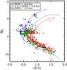 |
Fig. 4 Derived absolute magnitude MV versus (B − V) colour for the present sample of Galactic field stars and for the atmospheric parameters derived by the pipeline of Paper I and projected on the Y2 isochrones. The colour codes and the isochrones are the same as in Fig. 3. Typical error bars are represented for different regions of the H–R diagram. |
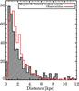 |
Fig. 5 In black we denote the distribution of the line-of-sight distances for the subset of the observed stellar sample that meet the quality criteria described in Sect. 5. Overplotted in red is the distribution of a randomly selected magnitude-limited (mV ≤ 18.5) sample of stars based on the Besançon catalogue. |
The availability of the distances (D) then allows us to estimate their
Galactic-centred Cartesian coordinates5
(XGC,YGC,ZGC):
 where
(X⊙,Y⊙,Z⊙)
= (8, 0, 0) kpc (Reid 1993) and l,
b are the Galactic coordinates.
where
(X⊙,Y⊙,Z⊙)
= (8, 0, 0) kpc (Reid 1993) and l,
b are the Galactic coordinates.
Table 4 presents the derived values and their associated errors (computed analytically, considering no errors on l and b). They will be used in Sect. 6 to assign a star to a particular Galactic component (thin disc, thick disc or halo).
Positions of the selected targets belonging to the final catalogue.
4.3. Kinematic properties and orbital parameters
Proper motions combined with distance estimates and radial velocities provide the
information required to calculate the full space motions of any star in the Galaxy. For
our sample the radial velocities were derived from the observed spectra (see Sect. 2), whereas magnitudes, colours and proper motions were
taken from Ojha et al. (1996). The associated
space-velocity components in the Galactic cardinal directions, U (towards
the Galactic centre), V (in the direction of the Galactic rotation) and
W (towards the north Galactic pole) were computed for all the stars
using the following equations:  where
μl and
μb are the proper motions on the sky6. We also computed the galactocentric velocities in a
cylindrical reference frame. In that case, the velocity components are
VR,
Vφ, and
VZ, with
VZ = W. They are
computed as follows:
where
μl and
μb are the proper motions on the sky6. We also computed the galactocentric velocities in a
cylindrical reference frame. In that case, the velocity components are
VR,
Vφ, and
VZ, with
VZ = W. They are
computed as follows: ![\begin{eqnarray} \label{eqn:vrho} V_R &=& \frac{1}{R} \left[ X_{\rm GC} \cdot (U+U_\odot) + Y_{\rm GC} \cdot (V+V_{\rm rot}+V_\odot) \right] \\ \label{eqn:vphi} V_\phi &=& \frac{1}{R} \left[ X_{\rm GC} \cdot (V+V_{\rm rot}+V_\odot) - Y_{\rm GC} \cdot (U+U_\odot) \right] , \end{eqnarray}](/articles/aa/full_html/2011/11/aa17373-11/aa17373-11-eq134.png) where
where
 is the planar radial coordinate with respect to the Galactic centre,
 km s-1 is the
solar motion decomposed into its cardinal directions relative to the Local Standard of
Rest (LSR, Dehnen & Binney 1998), and
Vrot = 220 km s-1 is the amplitude of the
Galactic rotation towards l = 90° and b = 0° (IAU 1985
convention; see Kerr & Lynden-Bell 1986).
In this reference frame a retrograde rotation is indicated by
Vφ > 0 km s-1.
km s-1 is the
solar motion decomposed into its cardinal directions relative to the Local Standard of
Rest (LSR, Dehnen & Binney 1998), and
Vrot = 220 km s-1 is the amplitude of the
Galactic rotation towards l = 90° and b = 0° (IAU 1985
convention; see Kerr & Lynden-Bell 1986).
In this reference frame a retrograde rotation is indicated by
Vφ > 0 km s-1.
The errors on these kinematic data are estimated as follows: for each star, we performed 5 × 10³ Monte-Carlo realisations for D, μl, μb and Vrad, assuming Gaussian distributions around their adopted values, with a dispersion according to their estimated errors. For every realisation, 6d phase-space parameters and angular momenta were computed, taking as a final value the mean of all realisations, and as an error the standard deviation (see Tables 4 and 1). The number of realisations was determined to achieve a stable result for each measurement. Later on, as described in Sect. 6.2, each of these Monte-Carlo realisations will be used to assign for each star a probability of belonging to one of the Galactic components.
The median estimated errors on the Galactic rotational velocities, Vφ, for metal-rich ([M/H] > −0.4 dex), intermediate metallicity (−1 < [M/H] < −0.4 dex) and low-metallicity ([M/H] < −1 dex) stars are of the order of 10, 18 and 48 km s-1, respectively. For VR we reach accuracies of 12, 23 and 49 km s-1, and for VZ we obtain 9, 16 and 41 km s-1, respectively.
Finally, from the present positions and space-motion vectors of the stars one can integrate their orbits up to several Galactic revolutions and hence estimate their orbital parameters. Stellar orbital eccentricities7, pericentric and apocentric distances were computed. For that purpose we considered a three-component Galaxy (dark halo, disc, bulge). The Milky Way potential was fixed, and modelled with a Miyamoto-Nagai disc, a Hernquist bulge and a logarithmic dark matter halo (see Helmi 2004, and references therein for more details).
Errors on these parameters were propagated from the previously found positions and velocities. Typical errors on eccentricities are ~22%. Results can be seen in Table 1 and in Fig. 6, where ϵ has been plotted versus [M/H]. As we will discuss in the next section, these eccentricities can be used to identify the Galactic components and distinguish the origins of the thick disc stars (Sales et al. 2009).
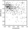 |
Fig. 6 Metallicity versus eccentricity for the 452 stars with full 6d phase-space coordinates. Typical errors are shown in the upper right corner. |
5. Star selection
We need the cleanest possible sample to confidently describe the properties of our observed stars. The final catalogue contains 479 stars, 452 of which have full 6d phase-space coordinates. Below we explain how they have been selected.
As already mentioned, from the initial 689 targets 53 stars that were identified as
binaries or had very low quality spectra were removed. In addition, we removed the targets
for which the parameters projected onto the isochrones clearly disagreed with the results of
the pipeline, according to the following criterion:
 (10)where
 and
and
 correspond to
the differences between the observed spectrum and the synthetic templates (resulting from
the pipeline parameters or those projected onto the isochrones, respectively). The above
condition removed 24 stars, mainly giants. In addition, 11 stars with a projection onto an
isochrone of 2 Gyr were removed from our survey because these young stellar populations are
expected neither in the thin disc (at those distance above the plane), the thick disc or the
halo. Removing these targets is justified, because the stars that are found to be so young
are clearly misclassified by the automatic pipeline (because of degraded spectral lines, bad
normalisation..., or because of the
log g-Teff degeneracy between the hot
dwarfs and the giants, see Paper I). In addition, this criterion also removes possible stars
on the blue horizontal branch (BHB), because the Y2 isochrones
closest to the BHB will be the youngest ones. Finally, we removed 11 stars for which the
spectra had an estimated error in the
Vrad > 10 kms-1, 43 stars with an
estimated error on D > 50%, and all remaining stars with
S/N < 20 pixel-1. Indeed, as shown
in Paper I, the errors in the atmospheric parameters, and hence on the distances are non
negligible in that case. As a matter of fact, with a selection for
S/N ≥ 20 pixel-1, errors less than 190 K,
0.3 dex and 0.2 dex are expected for thick disc stars for Teff,
log g and [M/H], respectively, leading to errors smaller than 35% on
the distances.
correspond to
the differences between the observed spectrum and the synthetic templates (resulting from
the pipeline parameters or those projected onto the isochrones, respectively). The above
condition removed 24 stars, mainly giants. In addition, 11 stars with a projection onto an
isochrone of 2 Gyr were removed from our survey because these young stellar populations are
expected neither in the thin disc (at those distance above the plane), the thick disc or the
halo. Removing these targets is justified, because the stars that are found to be so young
are clearly misclassified by the automatic pipeline (because of degraded spectral lines, bad
normalisation..., or because of the
log g-Teff degeneracy between the hot
dwarfs and the giants, see Paper I). In addition, this criterion also removes possible stars
on the blue horizontal branch (BHB), because the Y2 isochrones
closest to the BHB will be the youngest ones. Finally, we removed 11 stars for which the
spectra had an estimated error in the
Vrad > 10 kms-1, 43 stars with an
estimated error on D > 50%, and all remaining stars with
S/N < 20 pixel-1. Indeed, as shown
in Paper I, the errors in the atmospheric parameters, and hence on the distances are non
negligible in that case. As a matter of fact, with a selection for
S/N ≥ 20 pixel-1, errors less than 190 K,
0.3 dex and 0.2 dex are expected for thick disc stars for Teff,
log g and [M/H], respectively, leading to errors smaller than 35% on
the distances.
Figures 3 and 5 show the H–R diagram and the los distance distribution for the final catalogue, which contains 479 stars. For the 452 stars for which the proper motions were available, Fig. 7 illustrates their VR, Vφ, and VZ velocity components. The targets mainly span los distances from ~175 pc up to ~10 kpc (corresponding to a distance above the plane Z ~ 7.5 kpc), with only 11 stars reaching up to D ~ 32 kpc (Z ~ 24 kpc). As described in Sect. 4.1, these very distant stars are thought to have strongly overestimated distances (up to 30%), and hence one should be careful concerning the conclusions obtained for them. In addition, the excess of stars seen in the VZ versus VR plot of Fig. 7 towards negative VZ and VR is caused by small number statistics rather than a stellar stream.
 |
Fig. 7 Galactocentric velocities computed for the observed sample as defined in Sect. 5. Typical errors are represented in the upper right corners. The colour code according to the metallicity is the same as in Fig. 3. |
 |
Fig. 8 Metallicity versus distance above the plane (top), versus heliocentric radial velocity (Vrad, middle plot) and versus rotational velocity (Vφ, lower plot), for the considered sample. Mean estimated errors are represented for three different heights or metallicity ranges. |
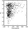 |
Fig. 9 Apparent magnitude versus derived heliocentric radial velocity (Vrad) of the entire sample. Empty circles represent the rejected targets, whereas the filled ones represent the selected stars for the final catalogue (see Sect. 5 for more details). Most of the faint targets with Vrad ≥ 180 kms-1 (typically, the halo stars) were removed. |
The metallicity clearly decreases with increasing Z (Fig. 8), as expected, because the proportion of thin disc, thick disc and halo stars changes. Nevertheless, we can notice in Fig. 8 a lack of metal-poor stars ([M/H] < −1.5 dex) at heights greater than ~3 kpc from the plane. One could argue that these missing stars are either misclassified, unobserved, or removed because of one of the quality criteria cited previously. The analysis of the magnitudes and the Vrad of the removed stars (empty circles in Fig. 9) shows that these targets are mainly faint stars (mv ≥ 18), with typical velocity values corresponding to the halo (Vrad ≥ 180 kms-1). This is strong evidence suggesting that some metal-poor stars have been observed, but were removed afterwards from the final catalogue. Indeed, the poor accuracies achieved for this type of stars (spectral signatures lost in the noise, see Paper I) lead to their removal when selecting a clean sample for the present analysis.
Finally, the Vrad distribution of the targets extends up to Vrad = +400 kms-1 (see Fig. 8). At these Galactic latitudes (b ~ 47°) Vrad ≳ 300 kms-1 corresponds to halo stars with retrograde orbits. The low metallicities of these stars combined with the derived Vφ-velocity component confirm this. These stars will be discussed in more detail in Sect. 6.2.3.
6. Characterisation of the observed stellar sample
To compare our observations with Galactic models, we created a catalogue of pseudo-stars with the same properties as ours. For that purpose we obtained a complete (up to mV = 19, mB = 20) catalogue of 8 × 10⁴ simulated stars towards our los from the website of the Besançon Galactic model8 (Robin et al. 2003). The latter supposes a thick disc formed through one or successive merger processes, resulting in a unique age population (11 Gyr) with a scale height of 800 pc, a local density of 6.2%, and no vertical gradients in metallicity or rotational velocity.
To run the model, we considered a mean diffuse absorption of 0.7 mag kpc-1. We applied parabolic photometric errors as a function of the magnitude, and a mean error on the proper motions of 2 mas year-1, according to the values given by Ojha et al. (1996). The input errors for the Vrad were those derived in Sect. 2. We selected stars with a Monte-Carlo routine to obtain the same mV and (B − V) distributions as in the FLAMES survey and the same ratio between giant and main-sequence stars (resulting from our final catalogue). This strict selection finally kept ~4 × 10³ simulated Besançon stars (called raw Besançon catalogue hereafter). Below we will first use this mock catalogue to help us in interpreting the vertical properties of the observed data (Sect. 6.1). Then, according to the hints given by the vertical study, the stars belonging to each Galactic component will be selected (Sect. 6.2), which will lead to a characterisation of the thin disc, thick disc and halo.
We recall that the model returns the Cartesian velocities U, V, W, and to obtain the values VR, Vφ in the cylindrical frame, one must use Eqs. (8) and (9). Both of them suppose a solar velocity and a galactocentric distance for the Sun. The values adopted by the Besançon model are not the commonly admitted ones (R⊙ = 8.5 kpc, U⊙ = 10.3 km s-1, V⊙ = 6.3 km s-1, W⊙ = 5.9 km s-1), and for that reason, we preferred to compare only the Cartesian velocities and not the best-suited cylindrical frame.
6.1. Study according to the distance above the Galactic plane
 |
Fig. 10 Comparisons between our observations (red dashed histograms) and the Besançon model predictions (black solid histograms) for the metallicities, rotational (V in Cartesian and Vφ in cylindrical coordinates system) and radial velocities. The left-side plots include the stars that are lower than 1 kpc, whereas the right-side plots include the stars farther than 1 kpc from the plane. Dotted black histogram corresponds to the raw Besançon model (as downloaded from the web, but biased to match our magnitude distribution), whereas the black continuous line corresponds to a model with a richer by 0.3 and 0.2 dex thick disc and halo, respectively. |
First, we divided the observed sample into stars lying closer and farther than 1 kpc from the Galactic plane, with 201 and 251 targets, respectively. We recall that this cut at Z = 1 kpc roughly corresponds to the scale height of the thick disc (Jurić et al. 2008) and to the threshold height above which Gilmore et al. (2002) identified a lagging population towards lower Galactic latitudes (b ~ 33°).
The left-side histograms of Fig. 10 represent a comparison between the model and the observations for metallicity, rotational velocity and Vrad of the closest stars. They show that the model reproduces the observations close to the plane fairly well, except for the position of the metallicity peak, for which we find a more metal-poor distribution, by 0.15 dex.
On the other hand, for the more distant set (right-side histograms), several adjustments
are needed to bring the metallicities and the velocities of the model to a better
agreement with the observations. Indeed, the model considers a thick disc and a halo
following Gaussian metallicity distributions, with a mean
![\hbox{$\overline{[M/H]}_{\rm TD}= -$}](/articles/aa/full_html/2011/11/aa17373-11/aa17373-11-eq171.png) 0.78 dex, and
0.78 dex, and
![\hbox{$\overline{[M/H]}_{\rm H}= -$}](/articles/aa/full_html/2011/11/aa17373-11/aa17373-11-eq172.png) 1.78 dex, respectively. These
values are too metal-poor compared to the mean thick disc and mean halo metallicities
found in the literature (see Soubiran et al. 2003;
Fuhrmann 2008; Carollo et al. 2010). We find that a thick disc and a halo more metal-rich than
the model default values by 0.3 dex and 0.2 dex respectively, lead to a much better
agreement of the metallicity distribution, as can be seen from the comparison between the
red dashed histogram (the observations) and the black one (the modified model) in the
first row plots of Fig. 10. We therefore propose
0.48 dex, and
1.58 dex. We stress that the
proposed value for the halo can suffer from the removal of some of the metal-poor stars,
as described in Sect. 5.
1.78 dex, respectively. These
values are too metal-poor compared to the mean thick disc and mean halo metallicities
found in the literature (see Soubiran et al. 2003;
Fuhrmann 2008; Carollo et al. 2010). We find that a thick disc and a halo more metal-rich than
the model default values by 0.3 dex and 0.2 dex respectively, lead to a much better
agreement of the metallicity distribution, as can be seen from the comparison between the
red dashed histogram (the observations) and the black one (the modified model) in the
first row plots of Fig. 10. We therefore propose
0.48 dex, and
1.58 dex. We stress that the
proposed value for the halo can suffer from the removal of some of the metal-poor stars,
as described in Sect. 5.
As far as the velocity distributions are concerned, the model still nicely represents the U and W distributions far from the plane, but not the velocity in the direction of Galactic rotation (V). Indeed, we find a shifted distribution with a peak around −70 km s-1, lower by 20 km s-1 compared to the predicted one. This ~20 km s-1 difference is also seen for Vφ, suggesting that its origin is not a spurious effect caused by the local, Cartesian reference frame. Nevertheless, this effect is hardly visible from the radial velocity distribution, and the lag is much less clear compared to that visible in Fig. 2 of Gilmore et al. (2002). This might be partly because at higher latitudes the contribution of V to the Vrad is less important.
To better characterise the observed sample, we studied the metallicity and the velocity distributions for narrower height bins up to 4 kpc from the plane. The size of the bins was chosen to include at least 20 stars. To fully take into account the uncertainties in the computed positions and metallicities of the observed stars, the plots of Fig. 11 were obtained from 5 × 10³ Monte-Carlo realisations on both parameters (i.e. D and [M/H]). For each realisation we computed the new velocities and measured the median metallicity and the median V of the stars inside each bin. The mean value and the 1σ uncertainties rising from the Monte-Carlo realisations were plotted. Finally, σv was obtained by computing the mean robust deviation of V inside each bin.
A clear change of regime is observed in Fig. 11 for [M/H], V and σV around 1 kpc, i.e. where the transition between the thin and the thick disc is expected. Closer than 1 kpc the metallicity trend is flat, whereas for the more distant stars a gradient ∂ [M/H] /∂Z = −0.14 ± 0.05 dex kpc-1 is measured. This gradient, agrees (within the errors) with that found by Katz et al. (2011) and Ruchti et al. (2011). Yet this gradient might be under-estimated because as noticed previously, our sample might be lacking low-metallicity stars at long distances. Velocity gradients of ∂Vφ/∂Z = 19 ± 8 km s-1 kpc-1 and ∂σVφ/∂Z = 9 ± 7 km s-1 kpc-1 are observed for the stars between 1 and 4 kpc, which agrees relatively well with the results found by Casetti-Dinescu et al. (2011) and Girard et al. (2006).
To better understand the origin of these trends, we used once more the Besançon model and
compared it to our observations. As suspected from the study above and below 1 kpc, the
raw Besançon model does not mimic our data correctly (Fig. 11, red diamonds). On the other hand, a more metal-rich thick disc and halo, and
a thick disc that lags behind the LSR by  km
s-1, as suggested previously, leads to a much better agreement between the
observations and the predictions (blue triangles). In particular, the measured trends seem
to be explained in our mock model as a smooth transition between the different Galactic
populations.
km
s-1, as suggested previously, leads to a much better agreement between the
observations and the predictions (blue triangles). In particular, the measured trends seem
to be explained in our mock model as a smooth transition between the different Galactic
populations.
Nevertheless, even with these adjustments the mock model does not represent all results we obtained. In particular, bins around Z = 1 kpc still clearly disagree, corresponding to the height where the thick disc is expected to become the dominant population. In addition, the plateau at the high-metallicity regime is not well modelled either, suggesting a local density of the thick disc higher than the one assumed for the model, correlated perhaps with a different scale height. Indeed, the model essentially predicts the number of thick disc stars seen above one scale height, and thus the adopted thick disc scale height and Z = 0 normalisation are degenerate.
Moreover, a clear correlation between Vφ and [M/H] is found for the stars between 0.8 and 2 kpc (∂Vφ/∂ [M/H] = −45 ± 12 km s-1 dex-1), in agreement with Spagna et al. (2010) and Lee et al. (2011), though in disagreement with the SDSS view of Ivezić et al. (2008), based on photometric metallicities. We recall that according to the radial migration scenarios (Roškar et al. 2008; Schönrich & Binney 2009), no or only a very small correlation is expected in the transition region, because the older stars that compose the thick disc have been radially well mixed.
 |
Fig. 11 Median metallicities and V-velocities at different height bins
above the Galactic plane. Each point has 1σ uncertainties, obtained
from 5 × 10³ Monte-Carlo realisations on the position of the stars (and
hence their velocities) and their metallicities. Red diamonds represent the
predictions of the raw Besançon model, whereas the blue triangles represent a
modified model with metal-richer thick disc and halo, and a thick disc that lags
behind the LSR by |

6.2. Characterisation of the Galactic components
We now aim to select the thin disc, thick disc and halo members to characterise these three Galactic components. We recall that there is no obvious predetermined way to define a sample of a purely single Galactic component. Any attempt will produce samples contaminated by the other populations.
We used the kinematic approach of Soubiran & Girard (2005); Bensby & Feltzing (2006); Ruchti et al. (2010) to select the stars belonging to each Galactic component (hereafter also called probabilistic approach). We recall that the advantage of this method is that no scale height is assumed for any population. The inconvenience is that it assumes a velocity ellipsoid, forcing in that way to find member candidates within the given dispersions (introducing for example biases in the eccentricity distributions because the cold stars like thin disc’s ones will have low eccentricities and very hot stars vey high eccentricities). This may lead to systematic misclassifications where the velocity distributionsoverlap, or if the assumed distributions are not the expected ones (i.e. non Gaussian or with significantly different means and/or dispersions).
In practice, for each set of U, V and
W a membership probability is computed according to the following
equation: 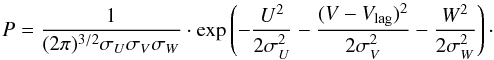 (11)The adopted values of
σU,
σV,
σW and Vlag
are the ones represented in Table 6. They are taken
from Bensby & Feltzing (2006), except for
the Vlag of the thick disc, in which case we used the value
suggested in Sect. 6.1 of −70 km s-1.
The probability of belonging to one of the components has to be significantly higher than
the probability of belonging to the others, to assign a target to it. In addition, one has
to take into account the uncertainties on the measured velocities, to avoid massive
misclassifications. In practice, instead of assigning a component based on the final
values of U, V and W (presented in
Table 4), we performed it for each of the
5 × 10³ Monte-Carlo realisations used to compute these values (see
Sect. 4.3). The adopted threshold in probability
ratio above which a realisation is assigned to a component was fixed to four (we checked
that our results are not affected by the adopted threshold, see below). The final
assignment was then made by selecting the component which occurred in most realisations.
(11)The adopted values of
σU,
σV,
σW and Vlag
are the ones represented in Table 6. They are taken
from Bensby & Feltzing (2006), except for
the Vlag of the thick disc, in which case we used the value
suggested in Sect. 6.1 of −70 km s-1.
The probability of belonging to one of the components has to be significantly higher than
the probability of belonging to the others, to assign a target to it. In addition, one has
to take into account the uncertainties on the measured velocities, to avoid massive
misclassifications. In practice, instead of assigning a component based on the final
values of U, V and W (presented in
Table 4), we performed it for each of the
5 × 10³ Monte-Carlo realisations used to compute these values (see
Sect. 4.3). The adopted threshold in probability
ratio above which a realisation is assigned to a component was fixed to four (we checked
that our results are not affected by the adopted threshold, see below). The final
assignment was then made by selecting the component which occurred in most realisations.
Adopted values for the characterisation of the Galactic components
Galactic population identification obtained from synthetic spectra of the Besançon sample simulated with a signal-to-noise ratio of approximately 20 pixel-1.
We tested this approach with the parameters obtained from the synthetic spectra of the Besançon sample, presented in Sect. 4.1. The adopted velocity ellipsoids are the same as in Table 6, but in that particular case, we chose a Vlag compatible with the model, of −46 km s-1. Results for spectra with S/N ~ 20 pixel-1 are shown in Table 7, where we checked the true membership of each assigned star (labelled (1)). This approach identifies the thin disc targets quite well (first column), but 25% of the thick disc candidates are actually thin disc members (third column). Furthermore, the majority of the identified halo stars are, in fact, thick disc members.
The assignment to a component for most of the stars is independent of the adopted probability threshold (in our case: four). Indeed, for the majority of the stars more than half of the Monte-Carlo realisations result in the same assignment. Increasing the probability threshold will only increase the realisations for which the assignment will not be obtained. Hence, the component which will have occurred in the majority of realisations will remain unchanged, keeping that way the same membership assignment. Finally, we stress that the results obtained when replacing the velocity ellipsoids of Bensby & Feltzing (2006) with those of Soubiran et al. (2003) or Carollo et al. (2010) remained identical. Indeed, the differences in the velocity ellipsoids or the rotational lag are not different enough (few km s-1) to introduce changes in the final candidate selection.
To obtain a sample of thick disc and halo stars as pure as possible, we found that a candidate selection based on the distance above the Galactic plane was preferred (like in Dierickx et al. 2010, for example). In this case, one has to adopt some values for the scale heights of each population, and a normalisation factor to estimate the pollution of the other components. Scale heights are a matter of debate, especially for the thick disc and the halo, but it is generally admitted that stars lying farther than ~1–2 kpc and closer than ~4–5 kpc from the Galactic plane are thick disc dominated (Siegel et al. 2002; Jurić et al. 2008; de Jong et al. 2010). Results obtained for the same Besançon sample with this distance selection are also shown in Table 7 under the label (2). In that case, only 15% of the thick disc stars are misclassified as thin disc members. In addition, the ratio of recovered halo targets has increased from 43% to 66% compared to the probabilistic approach.
Keeping these results in mind, we decided below, to investigate the results obtained by both methods (Z selection and probabilistic approach) for our observed data. We performed Gaussian fits of the distributions of U, V, W and [M/H] for each Galactic component, and we discuss the mean values and dispersions for each method. Results and their 1σ uncertainties are shown in Table 8.
The probabilistic approach assigned 154 stars to the thin disc, 193 stars to the thick disc and 105 stars to the halo. On the other hand, in the Z selection the 163 stars lying closer than Z = 800 pc were assigned to the thin disc, the 187 stars lying between 1 ≤ Z ≤ 4 kpc to the thick disc, and the 45 stars above 5 kpc from the plane to the halo.
6.2.1. The thin disc
The values found with the kinematic approach shown in Table 8 are consistent with the properties of the old thin disc (Vallenari et al. 2006; Soubiran et al. 2003, and references therein). The mean eccentricity for the thin disc stars is 0.14, with a dispersion of 0.06 (Fig. 13), though we remind the reader that these values are expected to be greater in reality. Indeed, the high eccentricity tail of the thin disc cannot be selected with the adopted procedure because of the biases introduced to the orbital parameters by the kinematic selection.
The most distant thin disc star is found at Z ~ 1874 ± 224 pc. We found one thin disc candidate with [M/H] ~ −1.5 dex, at Z ~ 250 pc. This star has Vrad = 1.3 ± 4.5 km s-1, which is typical of the thin disc. Nevertheless, we rather suspect this target to be thick disc member, whose kinematics occupy the wings of the thick disc distribution function in a region that overlaps the thin disc distribution function. This nicely illustrates the limitations of our adopted Gaussian model for the distribution functions. A measurement of its α-elements abundances would increase the dimensionality available for population classification, and so might help to identify its membership with confidence.
A selection according to Z-distance results in a hotter velocity ellipsoid and a lower mean metallicity compared to the kinematic selection. The higher lag and the lower metallicity found with this method is probably caused by the pollution from the thick disc. This is also suggested from the eccentricity distribution of Fig. 14, where one can notice that the thin disc has an anomalously high number of stars with ϵ ≳ 0.2. Indeed, we recall that in that case, stars up to Z = 800 pc are considered to be thin disc members. This model is of course dynamically unphysical, and is adopted here merely as a limiting and convenient case to illustrate different population classification outcomes. The contamination from the thick disc will thus depend mainly on the local density of the latter, whose values are found to vary in the literature from 2% up to 12% (see Arnadottir et al. 2009, for a review of the normalisation factors).
Considering a thin disc with  km s-1 (as
found with the kinematic approach) and a thick disc with
km s-1 (as
found with the kinematic approach) and a thick disc with
 km s-1, the
contamination caused by the latter should be ~19% to recover the lag of
~− 15 km s-1 that we measure. Roughly the same result (18%) is
obtained when looking for the amount of thick disc contaminators which is needed to pass
from
km s-1, the
contamination caused by the latter should be ~19% to recover the lag of
~− 15 km s-1 that we measure. Roughly the same result (18%) is
obtained when looking for the amount of thick disc contaminators which is needed to pass
from ![\hbox{$\overline{[M/H]}=-0.22$}](/articles/aa/full_html/2011/11/aa17373-11/aa17373-11-eq258.png) dex (kinematic
approach) to −0.27 dex (Z selection) with a canonical thick disc
metallicity of −0.5 dex.
dex (kinematic
approach) to −0.27 dex (Z selection) with a canonical thick disc
metallicity of −0.5 dex.
Because the kinematics are reasonably well established in the solar neighbourhood, we conclude for the thin disc that the probabilistic approach should return more robust results than the Z-distance selection.
6.2.2. The thick disc
The mean V-velocity ( km s-1,
 km s-1, see
Tables 8 and 9) found with the kinematic approach is slightly higher than the typical
canonical thick disc value, which less than −50 km s-1 (see, for example,
Wilson et al. 2011). The mean eccentricity is
0.33, with a dispersion of 0.13 (see Fig. 13). The
closest thick disc star is found at Z = 129 ± 10 pc, and the most
distant one at Z ~ 5.33 ± 1.17 kpc. We find that the
metallicity of the thick disc extends from ~−1.8 ± 0.1 dex up to
super-solar values of ~+0.25 ± 0.1 dex, and that
km s-1, see
Tables 8 and 9) found with the kinematic approach is slightly higher than the typical
canonical thick disc value, which less than −50 km s-1 (see, for example,
Wilson et al. 2011). The mean eccentricity is
0.33, with a dispersion of 0.13 (see Fig. 13). The
closest thick disc star is found at Z = 129 ± 10 pc, and the most
distant one at Z ~ 5.33 ± 1.17 kpc. We find that the
metallicity of the thick disc extends from ~−1.8 ± 0.1 dex up to
super-solar values of ~+0.25 ± 0.1 dex, and that
![\hbox{$\overline{[M/H]}=-0.41\pm0.02$}](/articles/aa/full_html/2011/11/aa17373-11/aa17373-11-eq267.png) dex. Let us note again that
the mean metallicity might be overestimated owing to the contribution of the thin disc
(misclassifications for the stars lying in the low velocity tails), and that the
kinematic selection introduces biases in the eccentricity distribution.
dex. Let us note again that
the mean metallicity might be overestimated owing to the contribution of the thin disc
(misclassifications for the stars lying in the low velocity tails), and that the
kinematic selection introduces biases in the eccentricity distribution.
On the other hand, the Z selection results in
 ,
,
 ,
,
 velocity distributions which are compatible with those found probabilistically9. Nevertheless, a slightly lower metallicity
(
velocity distributions which are compatible with those found probabilistically9. Nevertheless, a slightly lower metallicity
(![\hbox{$\overline{[M/H]}=-0.45$}](/articles/aa/full_html/2011/11/aa17373-11/aa17373-11-eq268.png) dex) is found, which,
interestingly, agrees well with the results suggested in Sect. 6.1, where we compared our results with those of the Besançon model.
dex) is found, which,
interestingly, agrees well with the results suggested in Sect. 6.1, where we compared our results with those of the Besançon model.
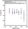 |
Fig. 12 V-velocity dispersion for different metallicity bins for the
stars lying between 1 < Z < 4 kpc above the plane.
Red diamonds represent the raw Besançon model, whereas the blue triangles
represent the model with our preferred model, which has a mean metallicity
−0.5 dex, and a mean Galactic rotational velocity
|

The argument that the thick disc is a distinct population compared to the thin disc is even more accredited by the plot of σV versus [M/H] (Fig. 12), obtained for the stars lying between 1 and 4 kpc. We see that for typical thick disc metallicities (−1 < [M/H] < −0.2 dex) the velocity dispersion is constant within the errors, around σV ~ 55 km s-1. At these heights and metallicities the pollution from the other components is expected to be very low (too high and too metal-poor for the thin disc, too low and too metal-rich for the halo). Hence, this plot seems to highlight the intrinsic velocity dispersion of the thick disc. But we cannot rule out the existence of an intrinsic vertical gradient in the metallicity and rotational velocity of the thick disc. Higher resolution spectroscopy and/or higher number of targets like the forthcoming Gaia-ESO survey will help to answer this question, though. A cleaner thick disc sample might be obtained by separating the thin disc from the thick disc based on the [α/Fe] ratio, and the halo from the thick disc by means of higher statistics.
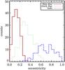 |
Fig. 13 Eccentricity distributions for the thin disc (in red), thick disc (in dotted green) and halo (in dotted-dashed blue). The candidates were selected based on their kinematics, according to the probabilistic approach of Ruchti et al. (2010). This selection therefore introduces biases in the eccentricity distributions because the tails of the velocity distributions cannot be selected. |
Finally, the orbital eccentricities of the thick disc obtained with the two methods have to be discussed (see Figs. 13 and 14). Very many authors have recognised that the shape of the eccentricity distribution can give valuable information about the formation mechanism of the thick disc and the accreted or not accreted origin of its stars (Sales et al. 2009; Di Matteo et al. 2011). Although for both selection methods the distribution tails can suffer from individual uncertainties or wrong population assignments, the position of the peak is reliable information according to these authors. The eccentricities in Fig. 13 suffer from selection biases, as discussed in the previous sections, because the membership was decided on kinematic criteria. Hence, no conclusions should be taken based on these results.
On the other hand, Fig. 14 suggests a peak at rather low values, around ϵ ~ 0.3. Hence, the pure accretion scenario, as in Abadi et al. (2003), which supposes a peak around ϵ ~ 0.5, can be ruled out (we note though that these results have been recently debated by Navarro 2011). Nevertheless, no separation can be made between the heating, migration or merger scenarios, which differ mainly in the detailed shape, especially in the breadth of the distribution.
We note, however, that Fig. 14 suggests a broader distribution than has been found so far for more local samples. This is very interesting because it might suggest that accretion has contributed slightly more compared to local sample, and that the dominant mechanism for the formation of the thick disc may well have varied with distance from the Galactic center.
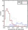 |
Fig. 14 Eccentricity distributions for the thin disc (in red), thick disc (in dotted green) and halo (in dotted-dashed blue). The candidates were selected based on their distance above the Galactic plane. |
6.2.3. The halo
The addition of the individual errors on Vrad, μl, μb and D leads to an unreliable selection of halo stars based only on their kinematics. Indeed, we recall that our tests conducted on synthetic spectra of the mock Besançon catalogue showed that a probabilistic assignment of halo membership inevitably generates a sample strongly polluted by the thick disc.
To minimise this pollution, our tests suggest to perform a selection on
Z instead. For the 45 stars being more distant from the plane than
Z = 5 kpc, the mean eccentricity is 0.69, with a dispersion of 0.16.
We find a mean metallicity of ![\hbox{$\overline{[M/H]} =-0.92\pm0.06$}](/articles/aa/full_html/2011/11/aa17373-11/aa17373-11-eq276.png) dex, with
σ [M/H] = 0.76 ± 0.06 dex.
These values are too metal-rich, compared to the commonly admitted value of
~− 1.6 dex for the inner halo (Carollo
et al. 2010). In addition, we find mean
velocities significantly different from zero, which is not expected. These odd values
are likely caused by the large uncertainty expected for the most distant stars for both
the distance and hence the velocities to our star selection criterion, which created a
biased and unreliable halo sample (see Fig. 9) and
probably to an underestimation of the errors for the proper motions for the most distant
stars (we recall that we assumed a constant error of 2 mas/year).
dex, with
σ [M/H] = 0.76 ± 0.06 dex.
These values are too metal-rich, compared to the commonly admitted value of
~− 1.6 dex for the inner halo (Carollo
et al. 2010). In addition, we find mean
velocities significantly different from zero, which is not expected. These odd values
are likely caused by the large uncertainty expected for the most distant stars for both
the distance and hence the velocities to our star selection criterion, which created a
biased and unreliable halo sample (see Fig. 9) and
probably to an underestimation of the errors for the proper motions for the most distant
stars (we recall that we assumed a constant error of 2 mas/year).
This could also explain the fairly large velocity dispersions that we find compared to those expected for the halo. For example, using SEGUE spectra, Carollo et al. (2010) found for the inner halo (σU,σV,σW) = (150 ± 2,95 ± 2,85 ± 1).
We note, however, that another possible solution to explain a part of this discrepancy can be found in Mizutani et al. (2003), who suggested that the retrograde stars in Gilmore et al. (2002) could be the debris of ω Cen. We searched among our retrograde stars for a possible identification of ω Cen candidates (e.g. in the metallicity space) without any success. Therefore we favour small-number statistics to explain these large velocity dispersions, although we cannot exclude their presence.
7. Derivation of the radial scale lengths and scale heights
Supposing that the thick disc and the thin disc are in equilibrium, the velocity ellipsoids
that were derived in the previous sections can be used with the Jeans equation to infer an
estimate of their radial scale lengths (hR) and
scale heights (hZ). Below we considered as thin
disc the stars below 800 pc from the Galactic plane, and as thick disc the stars between 1
and 3 kpc to avoid a strong contamination from the other components. In addition, the
dispersions of the velocity ellipsoids were corrected from the observational errors by
taking them out quadratically, as in Jones & Walker
(1988). In cylindrical coordinates the radial and azimuthal components of the Jeans
equation are 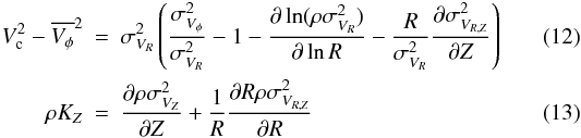 where
ρ is the density of the considered Galactic component,
Vc = 220 km s-1 is the circular velocity at the
solar radius, is
the mean rotational velocity of the stars having the
σVR,σVφ,σVZ
velocity dispersions,
where
ρ is the density of the considered Galactic component,
Vc = 220 km s-1 is the circular velocity at the
solar radius, is
the mean rotational velocity of the stars having the
σVR,σVφ,σVZ
velocity dispersions, 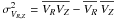 ,
and KZ is the vertical Galactic acceleration.
,
and KZ is the vertical Galactic acceleration.
7.1. Radial scale lengths
We consider that
ρ(R) ∝ exp(−R/hR),
and that  has the same
radial dependence as ρ (as in Carollo
et al. 2010). Therefore,
has the same
radial dependence as ρ (as in Carollo
et al. 2010). Therefore,  . In
addition, one can assume that
. In
addition, one can assume that  , which
is true if the Galactic potential is an infinite constant surface density sheet (Gilmore et al. 1989). In this case, the axes of the
velocity ellipsoid are aligned with the cylindrical coordinates, and Eq. (12) becomes:
, which
is true if the Galactic potential is an infinite constant surface density sheet (Gilmore et al. 1989). In this case, the axes of the
velocity ellipsoid are aligned with the cylindrical coordinates, and Eq. (12) becomes: 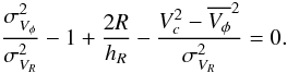 (14)An alternative
option is to consider that the Galactic potential is dominated by a centrally concentrated
mass distribution and that the local velocity ellipsoid points towards the Galactic centre
(Gilmore et al. 1989; Siebert et al. 2008). In that case, the previous term becomes
(14)An alternative
option is to consider that the Galactic potential is dominated by a centrally concentrated
mass distribution and that the local velocity ellipsoid points towards the Galactic centre
(Gilmore et al. 1989; Siebert et al. 2008). In that case, the previous term becomes
 (15)Eq.
(12) can then be rewritten as follows:
(15)Eq.
(12) can then be rewritten as follows:
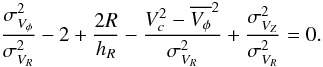 (16)Each of the terms of
Eqs. (14) or (16) were measured in our data, leaving as the
only free variable the radial scale length hR
of the discs. With the values derived for the thick disc of
(
(16)Each of the terms of
Eqs. (14) or (16) were measured in our data, leaving as the
only free variable the radial scale length hR
of the discs. With the values derived for the thick disc of
( km s-1, we find
hR = 3.6 ± 0.8 kpc using Eq. (14), and
hR = 3.4 ± 0.7 kpc using Eq. (16). These two values reasonably agree between
them, and are found in the upper end of the values cited in the literature (ranging from
2.2 kpc, Carollo et al. 2010, up to 3.6 kpc, Jurić et al. 2008; or even 4.5 kpc in the case of Chiba & Beers 2001).
km s-1, we find
hR = 3.6 ± 0.8 kpc using Eq. (14), and
hR = 3.4 ± 0.7 kpc using Eq. (16). These two values reasonably agree between
them, and are found in the upper end of the values cited in the literature (ranging from
2.2 kpc, Carollo et al. 2010, up to 3.6 kpc, Jurić et al. 2008; or even 4.5 kpc in the case of Chiba & Beers 2001).
Using Eq. (16) and
( km s-1, we find that
the thin disc has a similar radial extent within our uncertainties as the thick disc, with
hR = 2.9 ± 0.2 kpc. A smaller thin
disc has been suggested by other recent observations (see Jurić et al. 2008), but once more, the value we derived is at the upper end of
the previously reported values in the literature. Still, an extended thin disc like this
is plausible because our data mainly probe the old thin disc, which is likely to be more
extended than its younger counterpart.
km s-1, we find that
the thin disc has a similar radial extent within our uncertainties as the thick disc, with
hR = 2.9 ± 0.2 kpc. A smaller thin
disc has been suggested by other recent observations (see Jurić et al. 2008), but once more, the value we derived is at the upper end of
the previously reported values in the literature. Still, an extended thin disc like this
is plausible because our data mainly probe the old thin disc, which is likely to be more
extended than its younger counterpart.
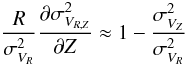
7.2. Scale heights
We assume that the last term of Eq. (13)
is negligible, because we are far from the Galactic centre, and that
ρ(Z) ∝ exp(−Z/hZ).
Equation (13) hence becomes 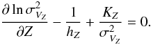 (17)We used
KZ = 2πG × 71 M⊙ pc-2
derived by Kuijken & Gilmore (1991) at
|Z| = 1.1 kpc, but we note that this value of
KZ might differ at the distances where
our targets are observed. We also used for the thick disc the value derived from our data
of
∂σVZ/∂Z = 15 ± 7 km
s-1 kpc-1 and
σVZ = 53 ± 3 km
s-1. Hence, for the thick disc, we find
hZ = 694 ± 45 pc.
(17)We used
KZ = 2πG × 71 M⊙ pc-2
derived by Kuijken & Gilmore (1991) at
|Z| = 1.1 kpc, but we note that this value of
KZ might differ at the distances where
our targets are observed. We also used for the thick disc the value derived from our data
of
∂σVZ/∂Z = 15 ± 7 km
s-1 kpc-1 and
σVZ = 53 ± 3 km
s-1. Hence, for the thick disc, we find
hZ = 694 ± 45 pc.
We found for the thin disc that ∂σVZ/∂Z = 19 ± 10 km s-1 kpc-1 and σVZ = 25 ± 1 km s-1, resulting in hZ = 216 ± 13 pc.
The derived values for both components agree well with, for example, Jurić et al. (2008), who suggested a thin disc with hZ = 300 pc, and a thick disc with hZ = 900 pc.
7.3. Metallicity dependence of the scale lengths of the thick disc
To investigate furthermore the metallicity gradients found for the rotational velocity of the thick disc, we computed the radial scale lengths and scale heights for different metallicity bins using Eqs. (16) and 17. The results are shown in Table 10, where the metallicity bins were selected to include at least 30 stars each. Though we found that both hR and hZ increased with decreasing metallicity (except for the most metal-poor bin), this trend is not strong enough to stand-out significantly from the errors. We conclude that within the errors, the same scale lengths and scale heights are found, which is the signature of only one population. Indeed, if a significant amount of relics of a destroyed massive satellite should exist in our line-of-sight, as suggested by Gilmore et al. (2002), one would expect them to have a different spatial distribution compared to the canonical thick disc, which we do not observe. Unless, of course, the satellite debris provides the dominant stellar population in the thick disc.
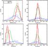 |
Fig. 15 Metallicity and velocity distributions for the Galactic components selected according to their position above the Galactic plane. The Gaussian fits were obtained taking into account the errors on each parameter with 5 × 10³ Monte-Carlo realisations. |
This result can also be discussed in the frame of a thick disc formed according to a radial migration scenario. In that case, the older stars that are at the solar radius have come from the inner parts of the Galaxy, and are expected to have a higher vertical velocity dispersion and a different metallicity, and hence, should exhibit scale heights dependent on metallicity. In particular, the model of Schönrich & Binney (2009) predicts a lower scale height for the metal-poor thick disc compared to its metal-rich counter part. This trend is not observed in our data (if it exists, it should be fairly small), which challenges the migration scenario as being the most important process of creation of the Galactic thick disc.
Kinematic parameters, radial scale lengths and scale heights for different metallicity bins of the thick disc targets.
8. Conclusions
A significant sample of roughly 700 low-resolution spectra (FLAMES/GIRAFFE LR8 setup, covering the IR Ca ii triplet) of stars faint enough to probe long distances and bright enough to get high S/Ns were collected towards the Galactic coordinates l ~ 277°, b ~ 47°. The stellar atmospheric parameters (Teff, log g, overall metallicity [M/H]) were extracted from the spectra with our automated code, which is fully described in Kordopatis et al. (2011). Given the proper motions of Ojha et al. (1996) and our derived radial velocities, we were able to derive the distances and the positions for 479 stars of our sample and the 3D motions and the orbital eccentricities for 452 of them.
We found a thick disc with a mean rotational velocity
 km
s-1, a value slightly higher than the commonly adopted lag of less than 50 km
s-1. We emphasise that our sample of stars probes distances above 1 kpc from
the plane, so this difference may imply a correlation between lag velocity and vertical
velocity rather than a simple inconsistency with local data. The mean measured metallicity
of the thick disc is −0.45 dex. Its metal-poor tails extends to −1.8 dex, whereas its
metal-rich tail goes up to solar and super-solar values. Depending on how the thick disc
stars are selected (Z positions or velocities), these values may vary a
little, but generally agree well between them. The vertical velocity gradient,
∂Vφ/∂Z = 19 ± 8 km s-1 kpc-1,
and metallicity gradient
∂ [M/H] /∂Z = −0.14 ± 0.05 dex kpc-1
that are measured for the regions where the thick disc is the dominant population
(1 < Z < 4 kpc) seem to agree well with a smooth transition
between the Galactic components, and are compatible with the values found by Chiba & Beers (2001); Allende Prieto et al. (2006); Girard
et al. (2006); Lee et al. (2011) and Ruchti et al. (2011), whose values range from 16 ± 4 to
30 ± 3 km s-1kpc-1 and from −0.07 ± 0.01 to
−0.09 ± 0.05 dex kpc-1. A correlation between the metallicity and the
rotational velocity of
∂Vφ/∂ [M/H] = 43 ± 11 km
s-1 dex-1 is also found, in agreement with Spagna et al. (2010) and Lee et al.
(2011).
km
s-1, a value slightly higher than the commonly adopted lag of less than 50 km
s-1. We emphasise that our sample of stars probes distances above 1 kpc from
the plane, so this difference may imply a correlation between lag velocity and vertical
velocity rather than a simple inconsistency with local data. The mean measured metallicity
of the thick disc is −0.45 dex. Its metal-poor tails extends to −1.8 dex, whereas its
metal-rich tail goes up to solar and super-solar values. Depending on how the thick disc
stars are selected (Z positions or velocities), these values may vary a
little, but generally agree well between them. The vertical velocity gradient,
∂Vφ/∂Z = 19 ± 8 km s-1 kpc-1,
and metallicity gradient
∂ [M/H] /∂Z = −0.14 ± 0.05 dex kpc-1
that are measured for the regions where the thick disc is the dominant population
(1 < Z < 4 kpc) seem to agree well with a smooth transition
between the Galactic components, and are compatible with the values found by Chiba & Beers (2001); Allende Prieto et al. (2006); Girard
et al. (2006); Lee et al. (2011) and Ruchti et al. (2011), whose values range from 16 ± 4 to
30 ± 3 km s-1kpc-1 and from −0.07 ± 0.01 to
−0.09 ± 0.05 dex kpc-1. A correlation between the metallicity and the
rotational velocity of
∂Vφ/∂ [M/H] = 43 ± 11 km
s-1 dex-1 is also found, in agreement with Spagna et al. (2010) and Lee et al.
(2011).
The radial scale length and scale height of the thick disc are estimated to be hR ~ 3.4 ± 0.7 kpc and hZ ~ 694 ± 45 pc, which agrees well with the SDSS results of Jurić et al. (2008). No clear metallicity dependences are detected for hR or for hZ, pointing towards a thick disc that is mainly composed by only one population.
Finally, we found a broad peak of the eccentricity distribution for the thick disc around ϵ ~ 0.3 which, according to the works of Sales et al. (2009) and Di Matteo et al. (2011) seem to rule out a pure accretion scenario. These results agree with those recently obtained by Wilson et al. (2011) and Dierickx et al. (2010), who measured the eccentricity distributions for a sample of RAVE and SEGUE stars.
However, several questions still remain open. For instance, we found difficulties in fitting the transition between the thin and the thick disc simply by adjusting parameters in the Besançon model. In addition, the plateau for the high-metallicity and low-altitude stars (i.e. the thin disc) seems to suggest a local density of the thick disc around 18%, higher than that assumed by that model. Finally, the existence of intrinsic vertical gradients in the thick disc cannot be ruled out, because we did not obtain a sufficiently well defined (and statistically large enough) sample of thick disc members. Additional targets to increase the statistics and higher resolution spectra on well selected spectral domains to separate thin disc stars from the thick disc ones with chemical content criteria are hence strongly recommended for future surveys.


Acknowledgments
The authors would like to thank the MESOCENTRE de l’Observatoire de la Côte d’Azur for computing facilities. We are grateful to M. Irwin for letting us use the routine of sky subtraction, A. Robin for her useful advice on the use of the Besançon model and the referee for his useful comments that improved the quality of our article. Finally, G.K. would like to thank the Centre National d’Études Spatiales (CNES) and the Centre National de Recherche Scientifique (CNRS) for the financial support. M.Z. acknowledges Proyecto Fondecyt Regular #1110393, The Fondap Center for Astrophysics 15010003, BASAL CATA PFB-06, and Programa Iniciativa Cientifica Milenio, awarded to The Milky Way Millennium Nucleus P07-021-F.
References
- Abadi, M. G., Navarro, J. F., Steinmetz, M., & Eke, V. R. 2003, ApJ, 591, 499 [NASA ADS] [CrossRef] [Google Scholar]
- Allen de Prieto, C., Barklem, P. S., Lambert, D. L., & Cunha, K. 2004, A&A, 420, 183 [NASA ADS] [CrossRef] [EDP Sciences] [Google Scholar]
- Allende Prieto, C., Beers, T. C., Wilhelm, R., et al. 2006, ApJ, 636, 804 [NASA ADS] [CrossRef] [Google Scholar]
- Arnadottir, A. S., Feltzing, S., & Lundstrom, I. 2009, in IAU Symp. 254, ed. J. Andersen, J. Bland-Hawthorn, & B. Nordström, 5 [Google Scholar]
- Battaglia, G., Tolstoy, E., Helmi, A., et al. 2006, A&A, 459, 423 [NASA ADS] [CrossRef] [EDP Sciences] [Google Scholar]
- Bensby, T., & Feltzing, S. 2006, MNRAS, 367, 1181 [NASA ADS] [CrossRef] [Google Scholar]
- Bergbusch, P. A., & Vandenberg, D. A. 1992, ApJS, 81, 163 [NASA ADS] [CrossRef] [Google Scholar]
- Bijaoui, A., Recio-Blanco, A., de Laverny, P., & Ordenovic, C. 2010, in ADA 6 – Sixth Conference on Astronomical Data Analysis [Google Scholar]
- Breddels, M. A., Smith, M. C., Helmi, A., et al. 2010, A&A, 511, A90 [NASA ADS] [CrossRef] [EDP Sciences] [Google Scholar]
- Brook, C. B., Kawata, D., Gibson, B. K., & Freeman, K. C. 2004, ApJ, 612, 894 [NASA ADS] [CrossRef] [Google Scholar]
- Carollo, D., Beers, T. C., Chiba, M., et al. 2010, ApJ, 712, 692 [NASA ADS] [CrossRef] [Google Scholar]
- Casetti-Dinescu, D. I., Girard, T. M., Korchagin, V. I., & van Altena, W. F. 2011, ApJ, 728, 7 [NASA ADS] [CrossRef] [Google Scholar]
- Chiba, M., & Beers, T. C. 2001, ApJ, 549, 325 [NASA ADS] [CrossRef] [Google Scholar]
- de Jong, J. T. A., Yanny, B., Rix, H., et al. 2010, ApJ, 714, 663 [NASA ADS] [CrossRef] [Google Scholar]
- Dehnen, W., & Binney, J. J. 1998, MNRAS, 298, 387 [NASA ADS] [CrossRef] [Google Scholar]
- Demarque, P., Woo, J.-H., Kim, Y.-C., & Yi, S. K. 2004, ApJS, 155, 667 [NASA ADS] [CrossRef] [Google Scholar]
- Di Matteo, P., Lehnert, M. D., Qu, Y., & van Driel, W. 2011, A&A, 525, L3 [NASA ADS] [CrossRef] [EDP Sciences] [Google Scholar]
- Dierickx, M., Klement, R., Rix, H., & Liu, C. 2010, ApJ, 725, L186 [NASA ADS] [CrossRef] [Google Scholar]
- Edvardsson, B., Andersen, J., Gustafsson, B., et al. 1993, A&A, 275, 101 [NASA ADS] [Google Scholar]
- Fuhrmann, K. 2008, MNRAS, 384, 173 [NASA ADS] [CrossRef] [Google Scholar]
- Gilmore, G., & Reid, N. 1983, MNRAS, 202, 1025 [NASA ADS] [CrossRef] [Google Scholar]
- Gilmore, G., Wyse, R. F. G., & Kuijken, K. 1989, ARA&A, 27, 555 [NASA ADS] [CrossRef] [Google Scholar]
- Gilmore, G., Wyse, R. F. G., & Norris, J. E. 2002, ApJ, 574, L39 [NASA ADS] [CrossRef] [Google Scholar]
- Girard, T. M., Korchagin, V. I., Casetti-Dinescu, D. I., et al. 2006, AJ, 132, 1768 [NASA ADS] [CrossRef] [Google Scholar]
- Helmi, A. 2004, MNRAS, 351, 643 [NASA ADS] [CrossRef] [Google Scholar]
- Ivezić, Ž., Sesar, B., Jurić, M., et al. 2008, ApJ, 684, 287 [NASA ADS] [CrossRef] [Google Scholar]
- Izzo, C., Kornweibel, N., McKay, D., et al. 2004, The Messenger, 117, 33 [NASA ADS] [Google Scholar]
- Jones, B. F., & Walker, M. F. 1988, AJ, 95, 1755 [NASA ADS] [CrossRef] [Google Scholar]
- Jurić, M., Ivezić, Ž., Brooks, A., et al. 2008, ApJ, 673, 864 [NASA ADS] [CrossRef] [MathSciNet] [Google Scholar]
- Katz, D., Soubiran, C., Cayrel, R., et al. 2011, A&A, 525, A90 [NASA ADS] [CrossRef] [EDP Sciences] [Google Scholar]
- Kerr, F. J., & Lynden-Bell, D. 1986, MNRAS, 221, 1023 [NASA ADS] [CrossRef] [Google Scholar]
- Kordopatis, G., Recio-Blanco, A., de Laverny, P., et al. 2011, A&A, 535, A106 [NASA ADS] [CrossRef] [EDP Sciences] [Google Scholar]
- Kuijken, K., & Gilmore, G. 1991, ApJ, 367, L9 [NASA ADS] [CrossRef] [Google Scholar]
- Lee, Y. S., Beers, T. C., An, D., et al. 2011, ApJ, 738, 187 [NASA ADS] [CrossRef] [Google Scholar]
- Lejeune, T., Cuisinier, F., & Buser, R. 1998, A&AS, 130, 65 [NASA ADS] [CrossRef] [EDP Sciences] [Google Scholar]
- Loebman, S. R., Roškar, R., Debattista, V. P., et al. 2011, ApJ, 737, 8 [NASA ADS] [CrossRef] [Google Scholar]
- Mizutani, A., Chiba, M., & Sakamoto, T. 2003, ApJ, 589, L89 [NASA ADS] [CrossRef] [Google Scholar]
- Navarro, J. 2011, in Assembling the puzzle of the Milky Way conference [Google Scholar]
- Navarro, J. F., Abadi, M. G., Venn, K. A., Freeman, K. C., & Anguiano, B. 2011, MNRAS, 412, 1203 [NASA ADS] [Google Scholar]
- Ojha, D. K., Bienayme, O., Robin, A. C., Creze, M., & Mohan, V. 1996, A&A, 311, 456 [NASA ADS] [Google Scholar]
- Recio-Blanco, A., Bijaoui, A., & de Laverny, P. 2006, MNRAS, 370, 141 [NASA ADS] [CrossRef] [Google Scholar]
- Reddy, B. E., Lambert, D. L., & Allen de Prieto, C. 2006, MNRAS, 367, 1329 [NASA ADS] [CrossRef] [Google Scholar]
- Reid, M. J. 1993, ARA&A, 31, 345 [NASA ADS] [CrossRef] [Google Scholar]
- Robin, A. C., Reylé, C., Derrière, S., & Picaud, S. 2003, A&A, 409, 523 [NASA ADS] [CrossRef] [EDP Sciences] [Google Scholar]
- Roškar, R., Debattista, V. P., Stinson, G. S., et al. 2008, ApJ, 675, L65 [NASA ADS] [CrossRef] [Google Scholar]
- Royer, F., Blecha, A., North, P., et al. 2002, in SPIE Conf. Ser. 4847, ed. J.-L. Starck, & F. D. Murtagh, 184 [Google Scholar]
- Ruchti, G. R., Fulbright, J. P., Wyse, R. F. G., et al. 2010, ApJ, 721, L92 [NASA ADS] [CrossRef] [Google Scholar]
- Ruchti, G. R., Fulbright, J. P., Wyse, R. F. G., et al. 2011, ApJ, 737, 9 [NASA ADS] [CrossRef] [Google Scholar]
- Ruck, M. J., & Smith, G. 1993, A&A, 277, 165 [NASA ADS] [Google Scholar]
- Sales, L. V., Helmi, A., Abadi, M. G., et al. 2009, MNRAS, 400, L61 [NASA ADS] [CrossRef] [Google Scholar]
- Schaller, G., Schaerer, D., Meynet, G., & Maeder, A. 1992, A&AS, 96, 269 [Google Scholar]
- Schlegel, D. J., Finkbeiner, D. P., & Davis, M. 1998, ApJ, 500, 525 [NASA ADS] [CrossRef] [Google Scholar]
- Schönrich, R., & Binney, J. 2009, MNRAS, 399, 1145 [NASA ADS] [CrossRef] [Google Scholar]
- Siebert, A., Bienaymé, O., Binney, J., et al. 2008, MNRAS, 391, 793 [NASA ADS] [CrossRef] [Google Scholar]
- Siegel, M. H., Majewski, S. R., Reid, I. N., & Thompson, I. B. 2002, ApJ, 578, 151 [NASA ADS] [CrossRef] [Google Scholar]
- Soubiran, C., & Girard, P. 2005, A&A, 438, 139 [NASA ADS] [CrossRef] [EDP Sciences] [Google Scholar]
- Soubiran, C., Bienaymé, O., & Siebert, A. 2003, A&A, 398, 141 [NASA ADS] [CrossRef] [EDP Sciences] [Google Scholar]
- Spagna, A., Lattanzi, M. G., Re Fiorentin, P., & Smart, R. L. 2010, A&A, 510, L4 [NASA ADS] [CrossRef] [EDP Sciences] [Google Scholar]
- Valdes, F., Gupta, R., Rose, J. A., Singh, H. P., & Bell, D. J. 2004, ApJS, 152, 251 [NASA ADS] [CrossRef] [Google Scholar]
- Vallenari, A., Pasetto, S., Bertelli, G., et al. 2006, A&A, 451, 125 [NASA ADS] [CrossRef] [EDP Sciences] [Google Scholar]
- Villalobos, Á., & Helmi, A. 2008, MNRAS, 391, 1806 [NASA ADS] [CrossRef] [Google Scholar]
- Wilson, M., Helmi, A., Morrison, H. L., et al. 2011, MNRAS, 413, 2235 [NASA ADS] [CrossRef] [Google Scholar]
- Wyse, R. F. G., Gilmore, G., Norris, J. E., et al. 2006, ApJ, 639, L13 [NASA ADS] [CrossRef] [Google Scholar]
- York, D. G., Adelman, J., Anderson, Jr., J. E., et al. 2000, AJ, 120, 1579 [Google Scholar]
- Zwitter, T., Castelli, F., & Munari, U. 2004, A&A, 417, 1055 [NASA ADS] [CrossRef] [EDP Sciences] [Google Scholar]
- Zwitter, T., Matijevič, G., Breddels, M. A., et al. 2010, A&A, 522, A54 [NASA ADS] [CrossRef] [EDP Sciences] [Google Scholar]
All Tables
Individual atmospheric parameters (as derived by the procedure of Paper I), relative V-Magnitudes, (B − V) colour, absolute V-magnitude and estimated S/N of the observed targets of the final catalogue.
Values at 70% of the error distribution for the recovered distances of the pseudo-stars of the Besançon model.
Galactic population identification obtained from synthetic spectra of the Besançon sample simulated with a signal-to-noise ratio of approximately 20 pixel-1.
Kinematic parameters, radial scale lengths and scale heights for different metallicity bins of the thick disc targets.
All Figures
|
Fig. 1 Radial velocity uncertainties versus the (B − V) colour for the final catalogue (479 stars), as selected in Sect. 5. Dots with different colours refer to different metallicity ranges. |
| In the text | |
|
Fig. 2 Apparent magnitude mv versus measured signal-to-noise ratio (per pixel) for all observed sample (689 stars in total). |
| In the text | |
|
Fig. 3 Atmospheric stellar parameters for the present sample of Galactic field stars derived by the pipeline of Paper I and projected onto the Y2 isochrones. Three isochrones for [M/H] = –1.5 dex and 13 Gyr (blue), [M/H] = –0.5 dex and 10 Gyr (green) and [M/H] = 0 dex and 7 Gyr (red) are represented. The metallicity values are those derived by the automated pipeline. Typical error bars are represented for different regions of the H–R diagram. |
| In the text | |
|
Fig. 4 Derived absolute magnitude MV versus (B − V) colour for the present sample of Galactic field stars and for the atmospheric parameters derived by the pipeline of Paper I and projected on the Y2 isochrones. The colour codes and the isochrones are the same as in Fig. 3. Typical error bars are represented for different regions of the H–R diagram. |
| In the text | |
|
Fig. 5 In black we denote the distribution of the line-of-sight distances for the subset of the observed stellar sample that meet the quality criteria described in Sect. 5. Overplotted in red is the distribution of a randomly selected magnitude-limited (mV ≤ 18.5) sample of stars based on the Besançon catalogue. |
| In the text | |
|
Fig. 6 Metallicity versus eccentricity for the 452 stars with full 6d phase-space coordinates. Typical errors are shown in the upper right corner. |
| In the text | |
|
Fig. 7 Galactocentric velocities computed for the observed sample as defined in Sect. 5. Typical errors are represented in the upper right corners. The colour code according to the metallicity is the same as in Fig. 3. |
| In the text | |
|
Fig. 8 Metallicity versus distance above the plane (top), versus heliocentric radial velocity (Vrad, middle plot) and versus rotational velocity (Vφ, lower plot), for the considered sample. Mean estimated errors are represented for three different heights or metallicity ranges. |
| In the text | |
|
Fig. 9 Apparent magnitude versus derived heliocentric radial velocity (Vrad) of the entire sample. Empty circles represent the rejected targets, whereas the filled ones represent the selected stars for the final catalogue (see Sect. 5 for more details). Most of the faint targets with Vrad ≥ 180 kms-1 (typically, the halo stars) were removed. |
| In the text | |
|
Fig. 10 Comparisons between our observations (red dashed histograms) and the Besançon model predictions (black solid histograms) for the metallicities, rotational (V in Cartesian and Vφ in cylindrical coordinates system) and radial velocities. The left-side plots include the stars that are lower than 1 kpc, whereas the right-side plots include the stars farther than 1 kpc from the plane. Dotted black histogram corresponds to the raw Besançon model (as downloaded from the web, but biased to match our magnitude distribution), whereas the black continuous line corresponds to a model with a richer by 0.3 and 0.2 dex thick disc and halo, respectively. |
| In the text | |
|
Fig. 11 Median metallicities and V-velocities at different height bins
above the Galactic plane. Each point has 1σ uncertainties, obtained
from 5 × 10³ Monte-Carlo realisations on the position of the stars (and
hence their velocities) and their metallicities. Red diamonds represent the
predictions of the raw Besançon model, whereas the blue triangles represent a
modified model with metal-richer thick disc and halo, and a thick disc that lags
behind the LSR by |
| In the text | |
|
Fig. 12 V-velocity dispersion for different metallicity bins for the
stars lying between 1 < Z < 4 kpc above the plane.
Red diamonds represent the raw Besançon model, whereas the blue triangles
represent the model with our preferred model, which has a mean metallicity
−0.5 dex, and a mean Galactic rotational velocity
|
| In the text | |
|
Fig. 13 Eccentricity distributions for the thin disc (in red), thick disc (in dotted green) and halo (in dotted-dashed blue). The candidates were selected based on their kinematics, according to the probabilistic approach of Ruchti et al. (2010). This selection therefore introduces biases in the eccentricity distributions because the tails of the velocity distributions cannot be selected. |
| In the text | |
|
Fig. 14 Eccentricity distributions for the thin disc (in red), thick disc (in dotted green) and halo (in dotted-dashed blue). The candidates were selected based on their distance above the Galactic plane. |
| In the text | |
|
Fig. 15 Metallicity and velocity distributions for the Galactic components selected according to their position above the Galactic plane. The Gaussian fits were obtained taking into account the errors on each parameter with 5 × 10³ Monte-Carlo realisations. |
| In the text | |
Current usage metrics show cumulative count of Article Views (full-text article views including HTML views, PDF and ePub downloads, according to the available data) and Abstracts Views on Vision4Press platform.
Data correspond to usage on the plateform after 2015. The current usage metrics is available 48-96 hours after online publication and is updated daily on week days.
Initial download of the metrics may take a while.